Efficient moving mesh methods for Q-tensor models of nematic liquid crystals

OF NEMATIC LIQUID CRYSTALS

CRAIG S. MACDONALD∗

, JOHN A. MACKENZIE∗

, ALISON RAMAGE∗

, AND

CHRISTOPHER J.P. NEWTON∗

Abstract. This paper describes a robust and efficient numerical scheme for solving the system of six coupled partial differential equations which arises when usingQ-tensor theory to model the behaviour of a nematic liquid crystal cell under the influence of an applied electric field. The key novel feature is the use of a full moving mesh partial differential equation (MMPDE) approach to generate an adaptive mesh which accurately resolves important solution features. This includes the use of a new monitor function based on a local measure of biaxiality. In addition, adaptive time-step control is used to ensure the accurate predicting of the switching time, which is often critical in the design of liquid crystal cells. We illustrate the behaviour of the method on a one-dimensional time-dependent problem in a Pi-cell geometry which admits two topologically different equilibrium states, modelling the order reconstruction which occurs on the application of an electric field. Our numerical results show that, as well as achieving optimal rates of convergence in space and time, we obtain higher levels of solution accuracy and a considerable improvement in computational efficiency compared to other moving mesh methods used previously for liquid crystal problems.

Key words. Nematic liquid crystals, adaptive moving meshes,Q-tensor model

AMS subject classifications.35K45, 65M50, 65M60

1. Introduction. Liquid crystals are intermediate states of matter which occur between the crystalline solid state and the isotropic liquid state, displaying some of the properties of both. Different liquid crystal phases may be classified by the amount and type of orientational and positional order of molecules within the material. Competition between the influences of bounding surfaces and the interaction between the permanent or induced electric dipoles of the liquid crystal molecules and an applied electric field can cause the material to switch between different orientational states, with the resulting change in optical characteristics allowing the material to be used in a Liquid Crystal Display (LCD). The ever-increasing presence of such LCDs in everyday life, in devices such as televisions, mobile phones, laptops, signage etc., means that the design of better displays is of real commercial interest, with a commensurate increase in the need for more effective numerical modelling tools. In this paper, we present a robust and efficient numerical scheme based on a finite element discretisation of a Q-tensor liquid crystal model on a moving mesh. We begin by presenting some background on these techniques.

1.1. Background. The most commonly-used continuum models for equilibrium orientational properties of liquid crystals represent state variables using one or more unit vector fields. In particular, the uniaxial nematic phase (the simplest and most common liquid crystal phase) is usually modelled using the director (a unit vector,

n, denoting the average orientation of the molecules in a fluid element at a point) and a measure of how ordered the molecules are in this direction, the scalar order parameter S (see, for example, [31]). For the uniaxial phase, this description is sufficient because the director is an axis of rotational symmetry. However, a more general biaxial configuration has no axis of complete rotational symmetry: in this case, a symmetric traceless second rank order parameter tensor,Q, is frequently used as the

∗

Department of Mathematics and Statistics, University of Strathclyde, Glasgow G1 1XH, Scot-land.

basis for mathematical modelling. In terms of identifying static equilibrium states, relatively unsophisticated numerical methods are often good enough (see, for example, [9, 16, 19, 23, 28, 29]). However, areas where distortion of the liquid crystal occurs over small length scales (between 10–100 nm) are of key importance, and it is crucial that the behaviour and nature of these so-calleddefects can be accurately represented by any numerical model. The presence in the physical problem of characteristic lengths with large scale differences (the size of the defect is very small compared to that of the cell which is about 1–10µm) suggests that more sophisticated numerical modelling techniques could be used here to great effect. In particular, one obvious approach is to use an adaptive grid, ensuring that there is no waste of computational effort in areas where there is no need for a fine grid.

There are several ways of introducing grid adaptivity to this type of problem. Using finite element discretisations with h (grid parameter) and p (degree of basis function) adaptivity has been explored in [8, 14, 15, 18]. There have also been several methods proposed which use adaptive moving meshes [1, 2, 25, 26]. It is now accepted that moving mesh methods are an efficient and effective means of resolving solutions that contain sharp features, such as boundary and interior layers, and localised so-lution singularities. Instead of refining or de-refining the mesh in areas of low or high solution error, the moving mesh method seeks to move existing mesh points so as to cluster them in areas of large solution error whilst maintaining the same mesh connectivity.

A common feature of the moving mesh studies listed above is the use of inter-polation to transfer the numerical solution between meshes as it is evolved in time. While this procedure is possible in one dimension, it is not easily extended to higher dimensions. In addition, the moving mesh methods used previously have been based on a discretisation of the well known mesh equidistribution principle. More recently, however, it has been accepted that greater control (and hence robustness) can be obtained using a moving mesh partial differential equation (MMPDE) [17]: this is the approach we adopt in this paper. Additional improvements on previously published studies include using a better adaptivity criterion together with a fully adaptive time-stepping procedure, leading to a more robust and accurate method overall. Most of the moving mesh papers above have studied the same test problem from Barberi et al. [3], namely, using a one-dimensional model to investigate the dynamics of the biaxial switching of a nematic Pi-cell subjected to a strong electric field, so we too will focus on this example (details are given in §1.2). As in [20], where we provided convergence results for a scalar model of a one-dimensional uniaxial problem, we also include a full numerical study of convergence properties of the algorithm. As well as showing optimal convergence in time and space (with quadratic finite elements), we also observe nodal superconvergence.

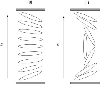
Fig. 1.1. Cell configuration with sample (a) horizontal and (b) vertical states under the influ-ence of an electric fieldE.

1.2. Test problem. In this paper, we consider a time-dependent switching pro-cess in a Pi-cell geometry which admits two topologically different equilibrium states. This so-called order reconstruction problem originates from attempts to model real phenomena first observed in laboratory experiments [3]. It has been used as a test example by previous authors interested in moving mesh methods techniques [1, 2, 26]. Although it has only one space dimension, it embodies many of the features of our real target applications, such as characteristic lengths with large scale differences in both space and time. As such, it provides a satisfactory proof of concept for our approach and allows us to illustrate the key features of our numerical methods in a relatively simple and uncluttered framework.

The geometry is that of a Pi-cell [7] of width one micron and the liquid crystal parameters used are taken from [3] (as described in _§2). At both boundaries, the cell surface is treated so as to induce alignments uniformly tilted by a specified tilt angle, θt(the angle between the director and the boundary surface), but oppositely

directed. This alignment is assumed to be fixed in time (giving what are known as strong anchoring boundary conditions). This allows two topologically different (uniaxial) equilibrium states: in one case, there is mostly horizontal alignment of the director with a slight splay and, in the other, there is mostly vertical alignment with a bend of almostπradians. Depending on the tilt angle and ratio of the elastic moduli of the liquid crystal material, either of these topologically-distinct states might have a lower elastic energy, but the energy barrier between them is always large enough to prevent a spontaneous transition. Representative configurations of both states are illustrated in Figure 1.1. In this paper, an electric field is applied and the transition between states when the applied voltage is sufficiently large is modelled. During the change from the horizontal to the vertical state, the liquid crystal passes temporarily through a biaxial phase: this progression is known asorder reconstruction.

2. Q-Tensor Model. For nematic systems in equilibrium, the globally stable phase of the system is the stationary point of the free energy functional with least free energy. In Landau-de Gennes theory [12], the free energy density is usually assumed to depend on the tensor order parameter Qand its gradient. We define this second rank order tensor by

Q= r

3 2

u_⊗u₋1 3I

,

where h· · · irepresents the local ensemble average over the unit vectorsu along the molecular axes andIis the identity. Note that including the factorp3/2 means that, for a uniaxial state with directornand scalar order parameterS, tr(Q2) =S2. One important advantage of the Q-tensor (as opposed to a director-based) description is that topological defects do not appear as mathematical singularities. The symmetric, traceless tensorQhas five degrees of freedom and hence we represent it as

Q= 



q1 q2 q3

q2 q4 q5

q3 q5 −q1−q4



, (2.1)

where each of the five quantitiesqi,i= 1, . . . ,5, is a function of time and the spatial

co-ordinates. In this setting, minimisation of the total free energy leads to a set of five coupled differential equations for the five degrees of freedom of Q. A detailed description of this model and its connection to the more traditional Frank-Oseen director-based model can be found in [21, 23].

In this paper, we are interested in distortions in the liquid crystal cell due to an applied electric field, so we may write the free energy as

F = Z

V

(Ft(Q) +Fe(Q,∇Q) +Fu(Q,∇Q)) dV +

Z

SFs (Q) dS,

where_Ft,Fe,FuandFsrepresent the thermotropic, elastic, electrostatic and surface

energy terms, respectively. Note that, in what follows, we will apply fixed bound-ary conditions (strong anchoring) so the surface energy term can be ignored in the minimisation. Taking the thermotropic energy,_Ft, up to fourth order in Qand the

elastic energy,_Fe, up to second order in the gradient ofQ, we obtain

Ft=

1

2A(T −T

∗_{) trQ}2 −

√ 6 3 B trQ

3

+1 4C(trQ

2

)2, (2.2a)

Fe=

1

2L1(divQ)

2₊1

2L2|∇ ×Q|

2_{, (2.2b)}

whereA,B, C,L1andL2are positive material constants,T represents temperature

and T∗ is the pseudocritical temperature at which the isotropic phase becomes un-stable (see [11]). The contribution to the bulk energy from the applied electric field, E say, can be written as

Fu=−

1

2ǫ0E·ǫE−Pf l·E, (2.2c)

whereǫ= ¯ǫI+ ∆ǫ∗_{Qis the dielectric tensor andǫ}

0is the permittivity of free space.

the scaled dielectric anisotropy, whereǫk andǫ⊥ denote the dielectric permittivities perpendicular and parallel to the long molecular axes, respectively. The flexoelectric contribution is taken to bePf l= ¯edivQ.

Denoting the bulk energy by_Fb=Ft+Fe+Fu, we may derive time-dependent

equations for the quantitiesqi in (2.1) using a dissipation principle (see, for example

[32] for a standard textbook form of the Euler-Lagrange-Rayleigh equations; an ex-tended formulation for continuum mechanics with specific reference to liquid crystals can by found in [30]). Here we use as a dissipation function

D=ν 2 tr

" ∂Q

∂t 2#

=ν( ˙q1q˙4+ ˙q21+ ˙q22+ ˙q32+ ˙q24+ ˙q25), (2.3)

whereνis a viscosity coefficient and the dot represents differentiation with respect to time [30, eq. (4.23)]. With spatial coordinates_{x1, x2, x3}, this leads to a system of

equations

∂_D ∂q˙i

=_{∇ ·}Γˆi−fˆi i= 1, . . . ,5, (2.4)

in the bulk [30, eq. (4.22)], where the vector ˆΓ_i has entries (ˆΓ_i)j=

∂Fb

∂qi,j

, qi,j=

∂qi

∂xj

, j= 1,2,3,

and ˆfi is given by

ˆ fi=

∂_Fb

∂qi

.

Note that the viscosity ν in (2.3) is related to Leslie’s rotational viscosity γ1 by

ν= (1/√3S2_)γ 1.

The electric field within the cell may be found by solving Maxwell’s equations. If we define an (unknown) scalar electric potentialU such thatE=_−∇U, this reduces to solving∇ ·D= 0, where the electric displacementDis given by

D=ǫ0(¯ǫI+ ∆ǫ∗Q)∇U+ ¯edivQ. (2.5)

On combining (2.4) and (2.5), after some manipulation, we arrive at the final system involving six coupled non-linear PDEs for qi, i= 1, . . . ,5, and the electric potential

U, given by

∂qi

∂t =∇ ·Γi−fi, i= 1, . . . ,5, (2.6a)

∇ ·D= 0, (2.6b)

where

Γ1= 1

3ν(2 ˆΓ1−Γˆ4), f1= 1

3ν(2 ˆf1−fˆ4),

Γ4= 1

3ν(2 ˆΓ4−Γ1ˆ ), f4= 1

and

Γi=

1

2νΓˆi, fi= 1

2νfˆi, i= 2,3,5.

As the focus of our study is the Pi-cell order reconstruction problem described in§1.2, from now on we restrict our attention to one space dimension, with a single spatial co-ordinatez. In this case, it can be shown that equations (2.6) reduce to

∂qi

∂t = ∂Γiz

∂z −fi i= 1, . . . ,5, (2.7a)

∂Dz

∂z = 0. (2.7b)

For computational purposes, we non-dimensionalise the equations in (2.7), scaling length with respect to the nematic coherence lengthζ=p9CL2/(2B2) and energies

by the quantity A(T−T∗). The values used for material constants throughout this paper are taken from [3], namely, L1 = 9.7×10−12 N, L2 = 2.4×10−12 N, A =

0.13×106 _JK−1_m−3_{, B = 1.6×10}6 _Jm−3_{, C = 3.9}

×106 _Jm−3_{, ǫ}

⊥ = 5, ǫk = 20 and ¯e =−27×10−12 _Cm−1

. These values are commensurate with a liquid crystal cell of the 5CB compound 4-cyano-4’-n-pentylbiphenyl and correspond to a nematic coherence length ofζ= 4.06 nanometres. The viscosity parameter isν = 0.1 Pa s.

3. Finite element method. With an MMPDE method, the finite element mesh moves as time evolves, but retains the same structure and connectivity. There are two main computational challenges: the governing physical PDEs need to be reformulated to account for the movement of the mesh, and a new adaptive mesh has to be generated at each time step. To tackle the first of these, it is convenient to introduce a family of bijective mappings _At such that, at time t, point ξ of a computational reference

configuration Ωc is mapped to point zof the current physical domain Ω. That is,

At: Ωc →Ω, z(ξ, t) =At(ξ). (3.1)

If a mappingg : Ω_→Ris defined on the physical domain, andT _⊆R+ represents the time domain, then the temporal derivative of g in the computational frame is defined as

∂g ∂t

ξ

: Ω_→R, ∂g ∂t

ξ

(z, t) = ∂ˆg

∂t(ξ, t), ξ=A −1 t (z),

where ˆg: Ωc×T →Ris the corresponding function in the computational frame, that

is, ˆg(ξ, t) =g(_At(ξ)). We also define themesh velocity z˙ as

˙

z(z, t) = ∂z ∂t

ξ

(A−1 t (z)).

In general, if a function q: Ω_→R is smooth enough, then applying the chain rule for differentiation gives

∂q ∂t

ξ

= ∂q ∂t

z

We can therefore reformulate (2.7) to take account of a moving mesh as follows: ∂qi ∂t ξ

−z˙ ∂qi ∂z =

∂Γiz

∂z −fi i= 1, . . . ,5, (3.2a)

∂Dz

∂z = 0. (3.2b)

Note that the main difference between (2.7) and (3.2) is the appearance of an addi-tional convection-like term which is due to the movement of the mesh.

3.1. Conservative weak formulation. To construct a weak formulation of (3.2) we consider a space of test functions ˆv_∈H1

0(Ωc). The mesh mapping (3.1) then

defines the test space

H0(Ω) =

v: Ω_→R:v= ˆv_{◦ A}t−1, ˆv∈H01(Ωc) .

A weak formulation of (3.2) can be now obtained using Reynolds’ transport formula. This states that, if ψ(z, t) is a function defined on Ω and Vt⊆Ω is such that Vt = At(Vc) withVc ⊆Ωc, then

d dt

Z

Vt

ψ(z, t) dz= Z Vt ∂ψ ∂t ξ

+ψ∂z˙ ∂z ! dz= Z Vt _∂ψ ∂t z +∂ψ ∂z z˙+ψ

∂z˙ ∂z

dz.

If functions ˆv ∈ H1

0(Ωc) in (3.1) do not depend on time, we can use this to deduce

that, for anyv∈ H0(Ω),

d dt

Z

Ω

vdz= Z

Ω

v∂z˙

∂zdz (3.3)

and

d dt

Z

Ω

vψdz= Z Ω v ∂ψ ∂t ξ

+ψ∂z˙ ∂z

!

dz. (3.4)

A conservative weak formulation can then be obtained by multiplying (3.2) by a test function v _{∈ H}0(Ω), integrating over Ω and using (3.3) and (3.4). IfHEq and HEU denote the approximation spaces with essential boundary conditions on qi and U,

respectively, then the resulting weak form is: find qi ∈ HEq(Ω), i = 1, . . . ,5, and U ∈ HEU(Ω) such that∀v∈ H0(Ω)

d dt

Z

Ω

qivdz−

Z

Ω

∂( ˙zqi)

∂z vdz= Z

Ω

Γiz

∂v ∂z dz−

Z

Ω

fivdz, (3.5a)

Z

Ω

Dz

∂v

3.2. Finite element semi-discretisation. We now assume that the reference domain Ωc is covered by a uniform partitionTh,cso that Ωc=∪I∈Th,cI. We will use N to denote the set of nodes of the finite element mesh and _Nint⊂ N to denote the

set of internal nodes. We also introduce the Lagrangian finite element spaces

Lk_(Ω

c) ={ˆvh∈H1(Ωc) : ˆvh|I ∈Pk(I), ∀I∈ Th,c} Lk

0(Ωc) ={ˆvh∈H1(Ωc) : ˆvh|I ∈ Lk(Ωc) : ˆvh= 0, ξ∈∂Ωc},

wherePk(I) is the space of polynomials on Iof degree less than or equal tok.

The mesh mapping (3.1) is discretised spatially using piecewise linear elements giving rise to a discrete mapping_Ah,t∈ L1(Ωc) of the form

zh(ξ, t) =Ah,t(ξ) =

N X

i=1

zi(t) ˆφi(ξ),

wherezi(t) =Ah,t(ξi) denotes the position of nodeiat timetand ˆφiis the associated

nodal basis function in _L1_(Ω

c). We denote the image of the reference interval Th,c

under the discrete mesh mapping _Ah,t byTh,t. The finite element spaces on Ω are

defined as

Lk_{(Ω) =}

{vh : Ω→R : vh= ˆvh◦ Ah,t−1, vˆ∈ Lk(Ωc)}, Hh,0(Ω) ={vh : Ω→R : vh= ˆvh◦ A−h,t1, vˆ∈ Lk0(Ωc)},

and Hh,Eq ⊂ L

k_{(Ω) and H}

h,EU ⊂ L

k_{(Ω) are the finite dimensional approximation}

spaces satisfying the Dirichlet boundary conditions for the qi’s and U, respectively.

With this notation, the finite element spatial discretisation of the conservative weak formulation (3.5) then takes the form: find qih(t) ∈ Hh,Eq(Ωt), i = 1, . . . ,5, and Uh∈ Hh,EU(Ω) such that∀vh∈ Hh,0(Ω)

d dt

Z

Ω

qihvhdz−

Z

Ω

∂( ˙zhqih)

∂z vhdz= Z

Ω

(Γih)z

∂vh

∂z dz− Z

Ω

fihvh dz, (3.6a)

Z

Ω

Dzh

∂vh

∂z dz= 0. (3.6b)

If the vectorq_i(t) contains the degrees of freedom definingqih, and the vectoru(t) the

degrees of freedom definingUh, then we may express (3.6a) as the system of non-linear

ordinary differential equations

d

dt(M(t)qi(t)) =Gi(t,qi(t),u(t)), i= 1, . . . ,5, (3.7a) where M(t) is the (time-dependent) finite element mass matrix. The discrete weak formulation of Maxwell’s equation (3.6b) results in the non-linear algebraic system

4. Moving the mesh. As mentioned above, there are two main issues that have to be addressed in order to use an adaptive moving mesh. We have already discussed how the governing physical PDEs need to be reformulated to account for the movement of the mesh: we presented a conservative weak reformulation of the Q-tensor equations in _§3.1, and the subsequent finite element semi-discretisation of these equations in_§3.2. We now discuss the procedure used to generate the adaptive mesh at each time step.

In one-dimensional moving mesh methods, the mesh is usually updated via a mesh generating equation based on theequidistributionof a positive monitor function. That is, grid points are selected in order to limit some measure of the solution error by distributing it equally across each subinterval. For this type of adaptivity, the new mesh is usually constructed as the image under a suitably defined mapping of a fixed mesh over an auxiliary domain. To illustrate this, we consider a generic 1D problem on the domain [0,1] with physical and computational coordinates denoted by z and ξ, respectively, and fixed boundary conditions at z = 0 and z = 1. We suppose a uniform mesh, given by ξi =i/N, i = 0,1, . . . , N (where N is a positive integer) is

imposed on the computational domain, and denote the corresponding mesh in Ω by

∆N ≡ {0 =z0< z1< . . . < zN−1< zN = 1}.

With this notation,

z=z(ξ, t), ξ∈Ωc= [0,1], t∈T,

denotes a one-to-one coordinate transformation between the domains. Given a func-tion representing a particular physical quantity from the problem,T(z, t) say, and an associatedmonitor functionρ(T(z, t)) (see§4.1), the one-dimensionalequidistribution principle can be expressed as

Z z(ξ,t)

0

ρ(_T(s, t)) ds =ξ Z 1

0

ρ(_T(z, t)) dz. (4.1)

Ramage and Newton [25] obtained an updated mesh based on a discretisation of the integrals appearing in (4.1) and the so-called de Boor algorithm [10]. Alternatively, a differential equation forz(ξ, t) can be obtained by differentiating (4.1) with respect toξto give

ρ(_T(ξ, t))∂z ∂ξ =

Z 1

0

ρ(_T(z, t) dz. (4.2)

A discretisation of (4.2) was used in the moving mesh method of Amoddeo et al. [1, 2]. However, one major drawback of using (4.1) or (4.2) is the lack of control of the grid trajectories. This can lead to instabilities in the resulting algorithms that can only be avoided by the use of excessively small time steps, which is clearly undesirable.

formulation of the equidistribution principle. Differentiating (4.2) with respect to ξ we get the equation

∂ ∂ξ ρ∂z ∂ξ

= 0. (4.3)

If the roles of the dependent and independent variables are swapped then, if (4.3) holds, in terms of the inverse mappingξ(x, t) we have

∂ ∂z 1 ρ ∂ξ ∂z

= 0. (4.4)

Note that (4.4) can also be interpreted as the Euler-Lagrange equation satisfied by the stationary points of the functional

I[ξ(z, t)] =1 2 Z 1 0 1 ρ ∂ξ ∂z 2 dz. (4.5)

An MMPDE can now be defined in terms of the gradient flow equation

∂ξ ∂t =−

1 τ δI δξ = 1 τ ∂ ∂z 1 ρ ∂ξ ∂z , (4.6)

whereτis a positive constant temporal smoothing parameter that controls how quickly the mesh reacts to changes inρ(_T(z, t)). Finally, swapping the roles of the dependent and independent variables, we arrive at the MMPDE

∂z ∂t = 1 τ ρ∂z ∂ξ −2 ∂ ∂ξ ρ∂z ∂ξ

, z(0, t) = 0, z(1, t) = 1. (4.7)

It is important to choose τ commensurate with the temporal scale of the problem under consideration: for all numerical experiments in_§6, we have set τ= 10−9_.

4.1. Monitor functions. Essential to the success of any moving mesh method is the choice of an appropriate monitor function. Previous studies have used the scaled solution arc-length (AL) monitor function

ρ(T(z, t)) = s

µ+ _∂

T(z, t) ∂z

2

, (4.8)

[25], and the Beckett-Mackenzie (BM1) monitor function

ρ(_T(z, t)) =α+

∂_T(z, t) ∂z 1 2

, α=

Z 1 0

∂_T(z, t) ∂z 1 2 dz, (4.9)

[1, 2], whereµandαare scaling parameters to be discussed below. In this paper we also consider the alternative monitor function [4]

ρ(T(z, t)) =α+

∂2 T(z, t)

∂z2 1 m

, α= max

( 1, Z 1 0 ∂2 T(z, t)

∂z2 1 m dz ) , (4.10)

evenly throughout the domain. This is desirable where there are multiple solution features that we wish to resolve accurately. In [4] it is shown that, for a function with a boundary layer, the optimal rate of approximation order using polynomial elements of degreepcan be obtained by ensuring that the parameterm_≥p+ 1. As we will use quadratic finite elements, we therefore requirem_≥3: we usem= 3 in all calculations. The parameterαis included in (4.9) and (4.10) to avoid mesh starvation external to layers. If α = 0, the resulting mesh would have almost all mesh points clustered within the layers as the monitor function outwith the layers (where solution gradients are small) would be close to zero. Note thatαis not a user-specified parameter, as its value is determined a posteriori from the numerical approximation itself. This is obviously more desirable than having a user-specified parameter, like µ in the AL monitor function (4.8). In practice, a lower bound is set onα to avoid undesirable oscillations in the mesh trajectories when gradients inT(z, t) are very small: in this paper, we useα= 1. Whenαis too small, errors introduced in approximatingT(z, t) are amplified and can cause the mesh to adapt incorrectly.

Having identified monitor functions, it remains to decide on an appropriate input function _T(z, t). In previous studies [1, 2, 25, 26], the authors set _T(z, t) =tr(Q2) which is known to vary rapidly in regions where order reconstruction occurs. Sub-sequently, it was shown by the present authors [20] that, for the uniaxial boundary value problem considered there, the ideal quantity on which to base the monitor func-tion is the scalar order parameter S (recall that, for a uniaxial state, tr(Q2) = S2). However, it is not immediately apparent that tr(Q2) is the ideal quantity on which to base a monitor function for problems involving biaxiality. In this paper, we therefore compare results computed using_T(z, t) =tr(Q2) with those computed using a direct measure of biaxiality. That is, we also use_T(z, t) =b(z, t), where

b(z, t) =

1₋6 tr(Q

3₎2

tr(Q2)3

12

(4.11)

is an invariant measure of biaxiality [3]. The range of this measure isb_∈[0,1], with uniaxial states corresponding to b = 0 and totally biaxial states corresponding to b= 1. In the experiments described in _§6, we use_T(z, t) =tr(Q2) with the AL and BM1 monitor functions (as studied in [1, 2, 25, 26]), and distinguish between our two variants of BM2 by using BM2a for (4.10) with_T(z, t) =tr(Q2), and BM2b for (4.10) with_T(z, t) =b.

A detailed analysis of the performance of a given monitor function would normally require asymptotic estimates of the behaviour of the solution close to significant fea-tures such as boundary layers and at defects. To our knowledge, no such estimates are available for theQ-tensor model when biaxiality effects are important, such as in the order reconstruction problem considered here. An analysis of the ability of monitor function BM1 and BM2 to resolve boundary layers in the absence of an electric field for a simpler purely uniaxial situation is given in [20]. Estimates of the thickness of possible boundary layers in the presence of magnetic fields in a uniaxial model can be found in [22]. Numerical simulations presented in [27] indicate that point defects typically occur over a length scale of a few nematic coherence lengths. The numer-ical results presented in §6 show that the monitor functions presented above are all capable of resolving these small scale structures.

similar to that originally proposed in [5] and [6]. One of the major advantages of decoupling the solution procedures is that it allows the flexibility of using different convergence criteria for the mesh and the physical solution. This is important, as it is well appreciated that the computational mesh is rarely required to be resolved to the same degree of accuracy as the physical solution.

We integrate forward in time in an iterative manner, solving for the grid and the physical solution alternatively. The following algorithm is used, where MAXPASS is the total number of passes allowed to reach a degree of convergence between successive estimates of the grid at the forward time level.

Set an initial uniform mesh ∆0

N. Set the initial guessq0i andu0.

Select an initial ∆t0. Setn= 0.

while(tn_{< t}max_);

pass = 0. ∆pass_N = ∆n

N,q pass

i =qni,upass=un. while(pass<MAXPASS);

O∆N = ∆passN .

Evaluate monitor function using ∆pass_N andqpass_i .

Integrate (4.7) forward in time to obtain new grid ∆pass+1_N . Integrate (3.7) forward in time to obtainqpass+1_i ,upass+1.

if (_||∆pass+1_{N −}O∆N||l∞ <Mtol),break;

pass = pass + 1.

end while

∆n+1 N = ∆

pass N , q

n+1 i =q

pass

i ,un+1 =upass.

n:=n+ 1.

end while

For efficiency, it is strongly desirable to only perform a small number of iterations at each time-step so we use MAXPASS = 4. If the grid converges quickly, the loop will be stopped before four passes have been completed. Note that one of the major advantages of using an MMPDE fully coupled with the PDEs from the physical prob-lem (as opposed to the static regridding type methods used in [1, 2, 8]) is that there is no need for any interpolation as the solution of the physical PDEs is approximated on the mesh at the forward time level.

5.1. Discretisation of the MMPDE. Although the MMPDE could also be discretised using a finite element method, here we use a finite difference approxi-mation (primarily for the convenience of adapting existing code). Specifically, we discretise (4.7) using second-order central differences on the uniform meshξi =i/N,

i= 0,1, . . . , N and obtain the semi-discrete system of moving mesh equations

˙ zi=

4

τ(˜ρi(hi+1+hi)) −2

˜ ρi+1

2hi+1−ρ˜i−12hi

. (5.1)

In (5.1), ˜ρi+1

2 is a smoothed monitor function defined as in [24] by

˜ ρi+1

2 =

Pi+p

k=i−pρk+1 2

q q+1

|k−i|

Pi+p

k=i−p

q q+1

|k−i| ,

The term ˜ρi is given by

˜ ρi=

˜ ρi−1

2(zi+12 −zi) + ˜ρi+12(zi−zi+12)

zi+1 2 −zi−12

,

where zi+1

2 =

1

2(zi+1+zi). The mesh at time level t = t

n+1 _{is computed using an}

implicit Euler approximation to (5.1).

5.2. Time integration. To integrate the physical equations (3.7a) forward in time, we employ a second-order singly diagonally implicit Runge-Kutta (SDIRK2) method similar to that used in [5]. This Runge-Kutta method is represented by the Butcher array

c A

bT

=

γ γ 0

1 1−γ γ

1₋γ γ

whereγ= (2₋√2)/2.

Integration of each equation in (3.7a) from t = tn _{to t = t}n+1 _{takes place via}

intermediate stagesKi,1 andKi,2 with

Mn+γKi,1= ∆tGi(t+c1∆t,(Mn+γ)−1Mnqni +a11Ki,1,un+γ)

Mn+1Ki,2= ∆tGi(t+c2∆t,(Mn+1)−1Mnqni +a21Ki,1+a22Ki,2,un+1) (5.2)

Mn+1_qn+1 i =M

n_qn

i +b1Ki,1+b2Ki,2,

where qn

i denotes the value of qi at time leveln and Mn is the finite element mass

matrix at time leveln. The intermediate stagesKi,1andKi,2are found using Newton

iteration. That is, forr= 1,2 we solve

"

Mn+cr_−a

rr∆t

_∂G

∂q_i p

qp i,r

#

Kp+1_{i,r −}Kp_i,r= ∆tG(t+cr∆t,qpi,r)−M

n+ci_Kp

i,r,

whereqp_i,r denotes the estimate ofq_i,r at thepth _{step of the Newton iteration, with}

qp_{i,r ≡}(Mn+cr₎−1_Mn_qn

i +ar1Kpi,1+ar2Kpi,2.

At thepth_{step of the Newton iteration we solve (3.7b) foru}p_{to updateuin (5.2). We}

note in passing that if we choose not to updateuafter each iteration of the Newton method, we find that the temporal convergence rates presented in_§6.1 are first order as opposed to second order. Newton’s method is terminated when_kKp+1_{i,r −}Kp_i,rk∞≤ Ktol. In the numerical experiments in§6 we set Ktol= 10−7.

In the course of integrating the solution forward in time, we employ adaptive time-stepping based on the computed solutions for q_i and on the solution of the MMPDE. To measure the solution error forq_iwe use the embedded first-order SDIRK approximation

ˆ

qn+1_i =qn_i + ∆tnKi,1,

which we obtain at no extra computational cost from the SDIRK2 scheme outlined in§5.2. The error indicator used is then

Ei=





N−1

X

j=0

(zn+1j+1 −zjn+1)

en+1_i,j +en+1i,j+1

2

!2



1 2

,

where

en+1_i,j =qn+1_{i,j −}qˆn+1_i,j .

Herezn

j denotes thejth node of the mesh at time leveln, andq n+1

i,j denotes the value

of thejth _{entry ofq}

iat nodejat time leveln+ 1. The time-step is then adapted via

the formula

∆tn+1_sol = ∆tn

×min maxfac,max "

minfac, η

_E

tol

maxi(Ei)

1₂#! .

In the computations in _§6, we set the tolerance Etol = 5×10−5, maxfac = 6.0,

minfac = 0.1 andη = 0.9. With these parameters, the mesh based control is similar to that of the computed solution. We measure the accuracy of a particular mesh using the quantity

gerr= max j=0,...,N|z

n+1 j −znj|.

The predicted time-step based on the mesh error is then given by

∆tn+1_mesh= ∆tn ×min

maxfac,max

minfac,log(gerr) log(gbal)

,

where we choose gtol= 0.5, gbal= 0.8×Mtoland Mtol= 5×10−2. The time-step at

the forward time level is then given by

∆tn+1= min ∆tn+1_sol ,∆tn+1_mesh .

A similar algorithm has previously been used successfully for solving the 1D viscous Burgers’ equation [5].

linearly between these two angles, as in the horizontal state in Figure 1.1. Initially, the biaxiality is negligible in the bulk, with two small amplitude (b _≈ 4_×10−2₎

boundary layers forming due to the boundary conditions. An electric field of strength 11.35 V µm−1 _{is applied parallel to thez-axis at timet}

on= 0.005 ms. The director

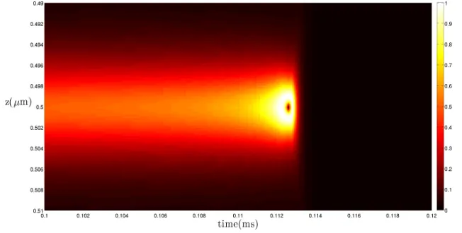
then begins to align vertically, parallel to the electric field, but is initially prevented from doing so, at the cell centre by the energy barrier and at the boundaries by the strong anchoring. Once the field is switched on, a thin layer forms in the biaxiality at the cell centre which, as time evolves, steadily increases in size until switching takes place. Figure 6.1 shows a blow-up of the complicated structure seen close to the switching timetswitch= 0.1125 ms for a grid of 256 quadratic elements using the

BM2b monitor function: the biaxiality at the cell centre has a volcano-like structure with a rim where b = 1 representing the purely biaxial state and a planar uniaxial point (b= 0) at the cell centre at the exact switching time. After the transition, the

Fig. 6.1.Contour plot of biaxiality at the cell centre with electric field strength 11.35V µm−₁

using the BM2b monitor function with256quadratic elements.

size of the biaxial wall at the cell centre rapidly decreases until b is again close to zero in the bulk and only the two boundary layers remain (again withb_≈4_×10−2_).

Finally, the field is switched off at time toff = 0.15 ms, after which the biaxiality at

the cell boundaries decreases further to an almost negligible level.

6.1. Convergence rates in space and time. In [20] we presented convergence results for a scalar model of a one-dimensional uniaxial problem. In a similar vein, we now investigate the convergence rates of both spatial and temporal errors for the much more complicated physical problem studied here. This would clearly be very difficult to do at the exact moment of switching, but we can still obtain valid results by choosing a pre-switching time for studying temporal convergence, and a time well after switching for studying spatial convergence (when the solution has entered a steady state).

As an analytical solution to this problem is not available, we compare our com-puted solutions with a reference solution obtained on a uniform mesh with 5000 quadratic elements and a uniform time-step ∆t= 10−9_{seconds. We will useq}

to denote this reference approximation toqi(z, t), and assume throughout that

|qi∗(z, t)−qi(z, t)| ≪ |qi∗(z, t)−qih(z, t)|.

Note that the results below areessentially independent of the type of reference grid used: calculations using fine reference grids based on the adaptive mesh methods give very similar results.

In what follows, we will denote the finite element approximation calculated on a grid withN quadratic elements byqih =qiN. The error in the approximationqiNwill

be denoted byeN

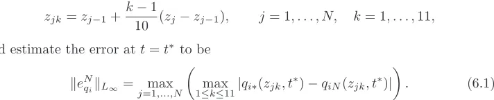
qi. To estimate theL∞ norm of the error, we subdivide each element using the 11 error sampling points given by

zjk=zj−1+

k₋1

10 (zj−zj−1), j= 1, . . . , N, k= 1, . . . ,11, and estimate the error att=t∗ _{to be}

keNqikL∞ = max j=1,...,N

max

1≤k≤11|qi∗(zjk, t

∗_)−q

iN(zjk, t∗)|

. (6.1)

Since the sampling points zjk will not in general coincide with the reference grid

points, the solution qi∗(zjk, t∗) is interpolated using the quadratic shape functions

and the local solution defined on the reference grid that includes the pointzjk. We

also estimate the spatial error in thel∞norm using the maximum error computed at the grid nodes, that is,

keN_q

ikl∞ = max

j=0,...,N|qi∗(zj, t

∗₎

−qiN(zj, t∗)|. (6.2)

We first consider convergence of the time discretisation scheme (for a fixed time-step ∆t). We estimate the error at time t∗ _{= 0.1024 ms, that is, before switching} has occurred. The values of (6.1) and (6.2) for q1, q3, q4 and U are presented in

Figure 6.2 for various values of ∆t (components q2 and q5 are exactly zero for this

problem). We see that, in both norms, the errors converge at a rate which isO(∆t−2) as we would expect when using a second order method to integrate forward in time. It is important to note that this optimal rate of convergence is only achieved if equation (3.7b) is solved for the electric potential at every Newton iteration. If, to increase efficiency,uis updated only after obtainingqn+1_i (that is, once per time-step) we only achieve first order convergence in time.

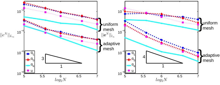
We now turn to estimating the rate of spatial convergence. We examine the error at timet∗ _{= 2 ms as by this time the solution has entered a steady state with only} boundary layers present in the biaxiality. The error norms (6.1) and (6.2) for the non-zero components ofQandU are presented in Figure 6.3 for various values ofN. For each norm, the results are shown for a uniform mesh and an adaptive mesh with monitor function BM2b. As expected, the errors associated with both types of grid appear to converge at the same asymptotic rate, but the constant involved is clearly smaller for the adaptive mesh. We observe that keN

qikL∞ appears to converge at the

rateO(N−3_{), which is the optimal rate expected using quadratic elements. However,}

the convergence rate of the error at the mesh nodes, that is, keN_qikl∞, appears to

be O(N−4_{). A similar convergence rate was observed in [20] for a one-dimensional}

5 6 7 8 9 10−11

10−10 10−9 10−8 10−7

log2∆t×10−9

||eN||_l ∞

2

1 q₁

q₃

q 4 u

5 6 7 8 9

10−11 10−10 10−9 10−8 10−7

log2∆t×10−9

||eN_|| L∞

2

1 q₁

q₃

q 4 u

Fig. 6.2.Temporal error convergence of approximations to the non-zero components ofQand the electric potential U at time 0.1024 ms using the BM2b monitor function with 256 quadratic elements. The electric field strength is 11.35V µm−₁

.

5 5.5 6 6.5 7

10−8 10−6 10−4 10−2

log2N

||eN_|| L∞

1

5 5.5 6 6.5 7

10−8 10−6 10−4 10−2

log2N

||eN||_l ∞

}

uniform mesh

adaptive mesh

adaptive mesh 1

3 4

}

}

}

q₁

q₃

q 4 u

q₁

q₃

q 4 u

Fig. 6.3.Spatial error convergence of approximations to the non-zero components ofQand the electric potentialU at time 2 ms. The curves labelledadaptive meshcome from using the BM2b monitor function on a grid with256quadratic elements, whereas those labelleduniform meshcome from using a uniform grid with 256 quadratic elements. The electric field strength is 11.35V µm−₁

.

back to Douglas and Dupont [13] who showed that for linear two-point boundary value problems, the standard Galerkin approximation using polynomial elements of degree pconverges in the L∞ norm at O(N−(p+1)), whereas the solution at the grid nodes converges at_O(N−2p_{). These convergence rates are consistent with our experiments,}

although it is somewhat remarkable to us that this property still holds when solving a system of highly non-linear PDEs as we have here.

BM1 ((4.9) with_T =tr(Q2)), BM2a ((4.10) with_T =tr(Q2)) and BM2b ((4.10) with T =b).

6.2.1. Switching time. One of the key challenges in the practical design of liquid crystal cells for displays is the accurate prediction of the switching time. In [25] the authors observe that the use of an over-coarse or poorly adapted grid can lead to poor prediction of switching times, or failure to capture switching altogether. We observe similar behaviour in Table 6.1, which presents the observed switching times using adaptive grids based on the four monitor functions under investigation plus a standard uniform grid. The electric field strength is 11.35 V µm−1_{: with this value,}

Table 6.1

Switching times (in milliseconds) for an electric field of strength11.35 Vµm−₁

.

Uniform Adaptive

N AL BM1 BM2a BM2b

64 no switching 0.1109 no switching 0.1248 0.1150

128 no switching 0.1108 0.1159 0.1127 0.1126

256 0.1205 0.1100 0.1126 0.1125 0.1125

512 0.1129 0.1109 0.1125 0.1125 0.1125

using our fine reference grid of 5000 uniform quadratic elements, we observe switching after 0.1125 milliseconds. For the coarseruniform gridsin Table 6.1, as anticipated, switching is missed altogether on the coarser grids, and the switching time has not quite converged for the grid sizes shown. With the BM1 monitor function, switching is again missed on the coarsest grid shown, but as the grid is refined, the switching time converges to 0.1125 ms. This is the same value found using both versions of the BM2 monitor function, although the latter grids require fewer points to correctly identify the switching time. This difference is due to the smoothness of the mesh trajectories (see_§6.2.2 below). With the AL monitor function, switching appears to occur slightly earlier (at timet= 0.1109 ms). This discrepancy can be explained by considering the effects of the adaptive time-stepping algorithm (see_§6.2.3 below). If a very small fixed time-step is used (∆t = 10−9_{), the switching time with the AL}

monitor function also converges to 0.1125 ms. We will therefore use this value as the correct value of the switching timetswitchfor the rest of our discussion.

6.2.2. Mesh trajectories. The trajectories for the adaptive grids obtained us-ing the four monitor functions above are shown in Figure 6.4. The red vertical lines indicate the times at which the electric field is switched on, when switching occurs, and when the field is switched off. In each case 256 elements have been used, al-though only every eighth node is plotted for clarity. We observe that, shortly after the electric field is switched on (t=ton), all four meshes adapt to resolve the large

solution gradients at both the cell centre and the cell boundaries. However, although the mesh generated using AL adapts well, it does so sharply; we also observe that mesh points move continuously in regions far from the cell centre and cell walls when ton < t < tswitch, even though solution gradients are small in these areas. These

0 0.1 0.2 0

0.2 0.4 0.6 0.8 1

(d)

time(ms) z(µm)

0 0.1 0.2

0 0.2 0.4 0.6 0.8 1

(c)

time(ms) z(µm)

0 0.1 0.2

0 0.2 0.4 0.6 0.8 1

(b)

time(ms) z(µm)

0 0.1 0.2

0 0.2 0.4 0.6 0.8 1

(a)

time(ms) z(µm)

t_switch t off t_on

Fig. 6.4.Node trajectories with 256 quadratic elements for monitor functions (a) AL, (b) BM1, (c) BM2a, (d) BM2b. The electric field strength is 11.35V µm−₁

.

discussed above. After switching, all of the meshes relax gradually (in the cases of BM1, BM2a and BM2b) or sharply (AL) at the cell centre due to the disappearance of the large solution gradient there. After the order reconstruction, but while the electric field is still switched on, the meshes are only adapted at the boundaries where layers remain due to competition between the electric field and the strong anchoring boundary condition. After the electric field is switched off (t=toff), we can see that

all meshes relax further at the boundaries.

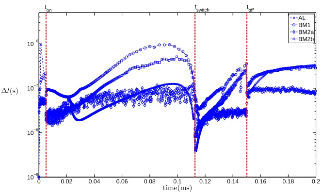
0 0.02 0.04 0.06 0.08 0.1 0.12 0.14 0.16 0.18 0.2 10−9

10−8 10−7 10−6

time(ms) ∆t(s)

t_on t_switch t_off

AL BM1 BM2a BM2b

Fig. 6.5. Evolution of the adaptive time-step for all four choices of monitor function with electric field strength 11.35V µm−₁

and256quadratic elements.

BM2b lead to meshes which adapt well to boundary and interior layers but the AL mesh does so much more rapidly, thus requiring smaller time-steps to be taken. As the mesh using BM2b adapts smoothly, larger time-steps can be used. In Table 6.2 we compare the total number of time steps needed using the various monitor functions.

Table 6.2

Comparison of the number of time steps used with256 quadratic elements and electric field strength 11.35V µm−₁

.

Monitor Function Time steps

AL 2140

BM1 635

BM2a 2175

BM2b 1409

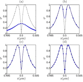
6.2.4. Biaxiality. Figure 6.6 shows a cross-section of the biaxiality at the cell centre when order reconstruction takes place. The reference fineuniformgrid solution is indicated by a dashed line. The approximations shown were computed at time t= 0.1125 ms using 256 quadratic elements with electric field strength 11.35V µm−1_.

0.4950 0.5 0.505 0.2

0.4 0.6 0.8 1

(a)

b

z(µm)

0 0.2 0.4 0.6 0.8 1

(b)

b

z(µm)

0.4950 0.5 0.505

0.2 0.4 0.6 0.8 1

(c)

b

z(µm)

0 0.2 0.4 0.6 0.8 1

(d)

b

z(µm)

Fig. 6.6. Cross-section of biaxiality at the cell centre when order reconstruction occurs for monitor functions (a) AL, (b) BM1, (c) BM2a and (d) BM2b, as compared with the reference fine grid solution (dashed line). All grids have 256 quadratic elements and the electric field strength is 11.35V µm−₁

.

importance of choosing an input function appropriate to the feature being modelled. We note also the slight asymmetry of the results obtained using all four monitor functions. This is in fact a physical effect caused by the flexoelectric term in the electric energy term (2.2) (symmetric solutions are obtained when ¯e= 0).

As the transition through biaxiality takes places, two eigenvalues ofQat the cell centre are exchanged. This exchange of eigenvalues is illustrated in Figure 6.7 (cf. [3, Figure 8]). This plot was produced using the BM2b monitor function with 256 quadratic elements. Analogous plots using the other three monitor functions tested here (AL, BM1 and BM2a) are indistinguishable from Figure 6.7 on this scale.

0 0.02 0.04 0.06 0.08 0.1 0.12 0.14 0.16 0.18 0.2 −0.2

−0.1 0 0.1 0.2 0.3 0.4

time(ms)

λ₁ λ

2 λ₃

Fig. 6.7. Eigenvalues ofQ at the cell centre with electric field strength 11.35V µm−₁

using the BM2b monitor function with256quadratic elements.

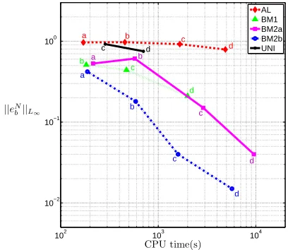
102 103 104

10−2 10−1 100

CPU time(s) ||eNb||L∞

a

a a

b

b b

b

c c c

c

c

d d d

d d

AL BM1 BM2a BM2b UNI

Fig. 6.8.L∞error in biaxiality plotted against the total CPU time in seconds for each method,

measured at time t= 0.1125 ms. The data points correspond to grids using 64 (a), 128 (b), 256 (c) and 512 (d) quadratic elements. Where no switching occurs, the corresponding point has been omitted.

functions based on tr(Q2), but using BM2b is better still.

In summary, it is clear that in order to calculatebto a given degree of accuracy, using the BM2b monitor function leads to the most accurate and efficient method. This is not surprising given that BM2b is based on input function (4.11) so is specif-ically tailored to model changes in biaxiality.

mesh where the equations have been discretised using second-order finite differences in space and first-order backward Euler time integration. To capture the highly non-linear nature of the Q-tensor equations, a conservative finite element discretisation using quadratic elements has been used to update the solution on the adaptive moving mesh. Time integration of theQ-tensor equations has been achieved using a second-order semi-implicit Runge-Kutta scheme and adaptive time-step control. These com-ponents have been put together to form an adaptive algorithm that has been carefully tested and the computed solutions have been shown to converge at optimal rates in both space and time. These experiments confirm our previous findings for a much simpler scalar problem, namely that it is not necessary to approximate the MMPDE equation with the same spatial or temporal degree of accuracy compared to that used to discretise the governing PDEs to ensure optimal rates of convergence [5]. Evidence has also been given to suggest that the computed solutions exibit nodal supercon-vergence, which is somewhat surprising given the highly non-uniform nature of the adaptive moving meshes. For the first time, a monitor function has been constructed based upon a local measure of biaxiality. This has been shown to lead to higher lev-els of solution accuracy and a considerable improvement in computational efficiency compared to those monitor functions used previously for liquid crystal problems.

We are currently extending our adaptive moving mesh method to solve liquid crystal problems in two and three dimensions. We are confident of rapid progress in this direction as the MMPDE approach and the conservative finite element discretisa-tion of the Q-tensor equations extend naturally to higher dimensions [6]. Challenges that lie ahead are the correct choice of adaptivity criteria for problems with moving singularities such as defects and the efficient solution of the large systems of highly non-linear algebraic equations arising after discretisation.

REFERENCES

[1] A. Amoddeo, R. Barberi, and G. Lombardo,Moving mesh partial differential equations to describe nematic order dynamics, Comput. Math. Appl., 60 (2010), pp. 2239–2252. [2] ,Electric field-induced fast nematic order dynamics, Liq. Cryst., 38(1) (2011), pp. 93–

103.

[3] R. Barberi, F. Ciuchi, G. Durand, M. Iovane, D. Sikharulidze, A. M. Sonnet, and E. Virga,Electric field induced order reconstruction in a nematic cell, Eur. Phys. J. E, 13 (2004), pp. 61–71.

[4] G. Beckett and J. Mackenzie,On a uniformly accurate finite difference approximation of a singularly perturbed reaction-diffusion problem using grid equidistribution, J. Comp. Appl. Math., 131 (2001), pp. 381–405.

[5] G. Beckett, J. A. Mackenzie, A. Ramage, and D. M. Sloan,On the numerical solution of one-dimensional PDEs using adaptive methods based on equidistribution, J. Comput. Phys., 167 (2001), pp. 372–392.

[6] ,Computational solution of two-dimensional unsteady PDEs using moving mesh meth-ods, J. Comput. Phys., 182 (2002), pp. 478–495.

[7] G. Boyd, J. Cheng, and P. Ngo,Liquid-crystal orientational bistability and nematic storage effects, Appl. Phys. Lett., 36 (1980), pp. 556–558.

[8] S. Cornford and C. J. P. Newton,An adaptive hierarchical finite element method for mod-elling liquid crystal devices, Tech. Rep. HPL-2011-143R1, Hewlett-Packard Laboratories, 2011.

[9] T. A. Davis and E. C. Gartland,Finite element analysis of the Landau-de Gennes mini-mization problem for liquid crystals, SIAM J. Numer. Anal., 35 (1998), pp. 336–362. [10] C. de Boor,Good approximation by splines with variable knots ii, in Conference on the

Ap-plications of Numerical Analysis, Dundee 1973, J. Morris, ed., vol. 363 of Lecture Notes in Mathematics, Springer-Verlag, Berlin, 1974.

[12] P. de Gennes,An analogy between superconductors and smectics A, Solid State Commun., 10 (1972), pp. 753–756.

[13] J. Douglas and T. Dupont,Galerkin approximations for two point boundary value problem using continuous, piece-wise polynomial spaces, Numer. Math., 22 (1974), pp. 99–109. [14] J. Fukuda and H. Yokoyama,Director configuration and dynamics of a nematic liquid crystal

around a two-dimensional spherical particle: Numerical analysis using adaptive grids, Eur. Phys. J. E, 4 (2001), pp. 389–396.

[15] J. Fukuda, M. Yoneya, and H. Yokoyama, Defect structure of a nematic liquid crystal around a spherical particle: adaptive mesh refinement approach, Phys. Rev. E, 65 (2002), p. 041709.

[16] E. C. Gartland, A. M. Sonnet, and E. G. Virga,Elastic forces on nematic point defects, Continuum Mech. Thermodyn., 14 (2002), pp. 307–319.

[17] W. Huang and R. Russell,Adaptive Moving Mesh Methods, Springer, New-York, 2011. [18] R. James, E. Willman, F. A. Fernandez, and S. E. Day,Finite-element modeling of

liquid-crystal hydrodynamics with a variable degree of order, IEEE Transactions on Electron Devices, 53 (2006), pp. 1575–1582.

[19] G.-D. Lee, J. Anderson, and P. Bos, Fast Q-tensor method for modelling liquid crystal director configurations with defects, Appl. Phys. Lett., 81 (2002), pp. 3951–3953.

[20] C. S. MacDonald, J. A. Mackenzie, A. Ramage, and C. J. P. Newton,Robust adaptive computation of a one-dimensional Q-tensor model of nematic liquid crystals, Computers and Mathematics with Applications, 64 (2012), pp. 3627–3640.

[21] H. Mori, J. E.C. Gartland, J. Kelly, and P. Bos,Multidimensional director modeling using the Q tensor representation in a liquid crystal cell and its application to the Pi cell with patterned electrodes, Jpn. J. Appl. Phys., 38 (1999), pp. 135–146.

[22] N. Mottram and S. Hogan,Magnetic field-induced changes in the molecular order in nematic liquid crystals, Continuum Mech. Thermodyn., 14 (2002), pp. 281–295.

[23] N. Mottram and C. J. P. Newton, Introduction to Q-tensor theory, Tech. Rep. 10/04, University of Strathclyde Department of Mathematics and Statistics, 2004.

[24] L. S. Mulholland, Y. Qiu, and D. M. Sloan,Solution of evolutionary partial differential equations using adaptive finite differences with pseudospectral post-processing, J. Comput. Phys., 131 (1997), pp. 280–298.

[25] A. Ramage and C. J. P. Newton,Adaptive solution of a one-dimensional order reconstruction problem in Q-tensor theory of liquid crystals, Liq. Cryst., 34(4) (2007), pp. 479–487. [26] ,Adaptive grid methods for Q-tensor theory of liquid crystals: A one-dimensional

feasi-bility study, Mol. Cryst. Liq. Cryst., 480(1) (2008), pp. 160–181.

[27] N. Schopohl and T. Sluckin,Defect core structure in nematic liquid crystals, Physics Review Letters, 59 (1987), pp. 2582–2584.

[28] N. Schopohl and T. J. Sluckin,Hedgehog structure in nematic and magnetic systems, J. Phys. France, 49 (1988), pp. 1097–1101.

[29] A. M. Sonnet, A. Kilian, and S. Hess, Alignment tensor versus director: Description of defects in nematic liquid crystals, Phys. Rev. E, 52 (1995), pp. 718–722.

[30] A. M. Sonnet and E. G. Virga,Dissipative Ordered Fluids: Theories for Liquid Crystals, Springer, New York, 2012.

[31] I. Stewart,The Static and Dynamic Continuum Theory of Liquid Crystals, Taylor & Francis, London, 2004.