The costs of adjusting labor: Evidence from temporally disaggregated data

City, University of London Institutional Repository

Citation

:

disaggregated data (11/10). London, UK: Department of Economics, City University London.

This is the unspecified version of the paper.

This version of the publication may differ from the final published

version.

Permanent repository link:

Link to published version

:

Copyright and reuse:

City Research Online aims to make research

outputs of City, University of London available to a wider audience.

Copyright and Moral Rights remain with the author(s) and/or copyright

holders. URLs from City Research Online may be freely distributed and

linked to.

City Research Online: http://openaccess.city.ac.uk/ publications@city.ac.uk

Department of Economics

The Costs of Adjusting Labor: Evidence from Temporally

Disaggregated Data

Firat Yaman

City University London

Department of Economics

Discussion Paper Series

No. 11/10

1 _{Department of Economics, City University London, Social Sciences Bldg, Northampton Square, London EC1V 0HB, UK.}

The Costs of Adjusting Labor: Evidence from Temporally

Disaggregated Data

Fırat Yaman∗

May 7, 2011

Abstract

I estimate the costs for establishments of hires and separations using a dynamic

la-bor demand framework and matched employer-employee data from Germany, which

records the exact dates of start and end of an employment spell. I estimate

ad-justment costs under different assumptions of adad-justment frequencies. Under the

assumption that establishments revise their labor demand every month, GMM

esti-mates suggest hiring costs per employee of approximately 5,000 Euros, and costs of

separations of 1,000 Euros. Hiring costs vary considerably between skilled (8,000 to

28,000 Euros per hire) and unskilled (4,000 to 8,000 Euros) labor. Spatial

aggrega-tion (large establishments) is associated with lower cost estimates, and only monthly

adjustment frequencies yield estimates consistent with theoretical predictions.

JEL classifications: C23; D22; J23

Keywords: Adjustment costs; Labor demand; Temporal aggregation

∗

City University London; Department of Economics; Whiskin St; London, EC1R 0JD. Phone:+44

(0)20 7040 8539. E-mail: Firat.Yaman.1@city.ac.uk. This paper was written as part of the Marie Curie

Research Training Network on ‘Transnationality of Migrants’ TOM, which is funded by the European

Commission through the Human Resources and Mobility action of its Sixth Framework Programme (EC

Contract No. MRTN-CT-2006-035873). I am indebted to my thesis supervisors Jason Abrevaya and

1

Introduction

Estimating the costs associated with adjusting employment is a notoriously difficult

en-deavor. In particular, three difficulties in estimating adjustment costs have been

ubiqui-tous. Can we infer anything about the structure of adjustment costs from data above the

plant or firm unit, say from sectoral data? The answer, it turns out, is no, a point made

most forcefully in Hamermesh (1989), where employment fluctuations aggregated over

just 7 plants suggest frequent and incremental adjustment, while the individual plants

exhibit intermittent adjustment. Only the former would be compatible with a purely

convex cost structure of adjustment. The wide availability of micro-data now easily

solves this problem. The second difficulty – temporal aggregation – is more difficult to

tackle (see Hamermesh (1993)). We can reasonably assume that the appropriate unit to

look at is the individual firm or plant, but at what frequency it revises its labor demand

is unclear. One may look at the time period that elapses between two adjustments, but

the employer or manager might have decided any number of times not to adjust within

that period. Most data used in the literature dictate what time frame is used by the

frequency of its waves, mostly quarterly or annual. This paper is distinct in the labor

adjustment literature in using matched employer-employee data which identify the exact

point of time of every employment flow into and out of an establishment, thus allowing

the use of any adjustment frequency, from daily to annual. Out of four different time

specifications (monthly, quarterly, half-annual, annual), I find that only the monthly

results are compatible with a dynamic labor demand model allowing for asymmetric

adjustment costs similar to the ones used in the literature. Finally, the third difficulty

has been getting actual point estimates of the money-value of costs. Many studies have

focused on inference of the structure of costs, but were not able to identify cost values

due to identification issues (e.g. only parameters normalized by residual variances were

identified), a recent example being Nilsen et al. (2006).

Despite these difficulties finding ways to estimate and infer adjustment costs is a

questions: Why did unemployment surge in the US but not in Germany during the 2009

recession, despite comparable contractions in GDP? Do we expect the labor market to

adjust through wages or employment, and how is unemployment affected when adjusting

employment is costly? Are technological parameters of production functions estimated

consistently when adjustment costs are not accounted for? In any case, when modeling

adjustment costs one needs to start with some idea of how they are incurred (are they

fixed or variable, symmetric or asymmetric?), of their magnitude, and of the frequency

of adjustment by employers. All of those issues have been reflected on earlier, and

Hamermesh and Pfann (1996) provide a review of the earlier literature.

Typically the identification of fixed and/or non-convex adjustment costs has been

achieved by exploiting the periods of inactivity and using some kind of latent variable

model to maximize a likelihood function on the probabilities of expansion and contraction

(Hamermesh (1989), Hamermesh (1992), Nilsen et al. (2006), and Varej˜ao and

Portu-gal (2007) using a hazard function estimation). The difficulty of this approach is how

exactly the thresholds between the different regimes should be specified. Abowd and

Kramarz (2003) provide the most direct method of estimating adjustment costs, using

reported costs and employment changes using a cross-section of French establishments.

Reported costs are regressed on a quadratic of hires and separations, where the constant

is interpreted as fixed costs, and the coefficient on the quadratic as a measure of the

convexity of costs. This has the advantage of circumventing temporal aggregation issues,

but can capture only measured/recorded and reported costs. They find substantial costs

of terminations, the fixed component often estimated at more than 150,000 Euros (1992

values). Hall (2004) uses annual sectoral data and identifies convex adjustment costs by

the response of factor input ratios to factor price ratios. In the presence of adjustment

costs, input ratios should be less responsive to changes in price ratios. Estimation results

cast some doubt on this method, since the coefficients carry “wrong” signs for 10 out

of 18 sectors (being estimated imprecisely, Hall interprets those asno costs for the said

industries). Finally, Caballero et al. (1997) and Cooper et al. (2004) exploit information

adjustment costs, the former relying on a theoretical and possibly wrongly measured

con-struct (the “gap” between desired and actual employment), and the latter using iterative

methods with the full dynamic problem of the establishments being solved numerically

at every step of the iteration. While the latter approach maps closely from theory to

estimation, it is computationally intensive and difficult to extend to more complicated

cases, such as the inclusion of different types of labor.

This paper uses generalized method of moments estimation of the first-order-condition

of the dynamic labor demand problem of an establishment. While GMM has become a

standard application to dynamic panel models, to my knowledge it has not been applied

in the adjustment cost framework. It has the advantage of being easily extended to

heterogeneous labor applications by simply estimating as many first-order-conditions as

there are factor inputs. All of the three difficulties mentioned above are – to some extent

– dealt with. I obtain and compare results under different assumptions of adjustment

frequencies, and coefficients for a model with constant marginal adjustment costs can be

interpreted as Euro-costs per employee.

2

Framework

The establishment maximizes its expected present value of current and future profits by

choosing how much labor to employ today, taking as given all prices. That decision will

matter for its labor demand in the next period, because the cost of changing employment

tomorrow will depend on employment today. This is intuitive and easy to see in a

recursive formulation:

V(lt−1,It) = max lt

ptq(lt)−wt·lt−c(lt−1,lt) +βEV(lt,It+1) (1)

Here c is the cost of adjusting labor, w is a wage vector for different kinds of labor.

Labor types will be indexed by j, and I assume that adjustment costs are separable for

types of labor: c = P

information (I) that will be revealed at the beginning of next period, including wages,

prices, productivity, and demand. The establishment enters the period with its

employ-ment from the previous period, it observes this period’s wages, prices, etc. and decides

how many new employees to employ. Importantly, adjustments are NET adjustments.

There are two reasons for this: The first is theoretical. In the framework above it makes

no sense for the establishment to hire and separate from one labor type in the same

period, since every worker of a certain type is assumed to be equal. Second, comparing

small and big establishments will provide some information on how aggregation within an

establishment affects estimates of adjustment costs. Big establishments can be thought

of as consisting of subdivisions, some of which might expand, and others contract within

the same time period. Costs will be incurred, but in the aggregate no adjustments will

be recorded. For small establishments net adjustment will coincide with gross

adjust-ment most of the time. To be sure, legal and technological differences between small

and big establishments make it impossible to attribute differences in estimates solely to

aggregation effects, and results should be interpreted as suggestive. A priori I would

hypothesize that adjustment is more costly for larger establishments, because large

es-tablishments are subject to stricter legal rules concerning labor adjustment and relations.

Furthermore, they probably command and employ more resources in the hiring process.

However, if adjustment costs are linear (a discussion of German labor relations and

differ-ent cost specifications follows below), and aggregation will suggest frequdiffer-ent adjustmdiffer-ent,

the marginal cost of adjustment is likely to be underestimated. Aggregation and

struc-tural/institutional factors would work in opposite directions, so that smaller estimates

for larger establishments would be conservative evidence for aggregation bias.

To keep the exposition simple, I solve equation (1) with one type of labor in the main

2.1 Convex costs

To start with the simpler model, I first derive labor demand for a convex adjustment cost

function from Hamermesh and Pfann (1996) allowing for asymmetric costs for hiring and

separations:

c(lt−1, lt) =

a

2(lt−lt−1)

2_−b(l

t−lt−1) + exp(b(lt−lt−1))−1

Ifb >0, the marginal cost of a positive adjustment exceeds that of a negative adjustment,

and vice versa if b < 0. Solving (1) with this is simple, since the value function is

differentiable. Using the envelope theorem I get

ptqt0−wt−a(lt−lt−1) +b(1−β)−beb(lt−lt−1)−βalt

+βE

alt+1+beb(lt+1−lt)

= 0

Assume thatE(lt+1|lt) =lt. Given all information today, let the establishment treat next

period’s optimal labor demand as a random variable distributed normally with meanlt.

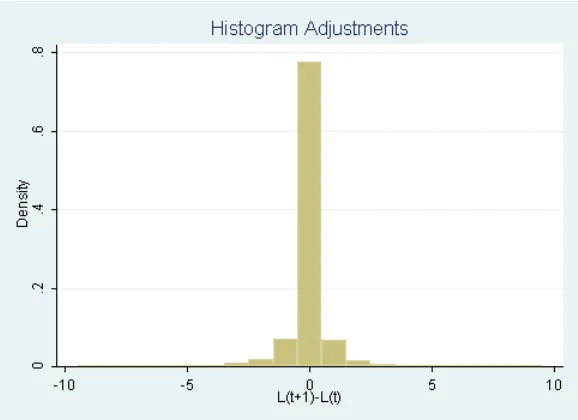
Figure 1 plots a histogram of lt+1 −lt. The distribution is symmetric around zero,

lending some justification for this assumption. Then eblt+1 _{is distributed log-normally}

withE(eblt+1_{) =e}blt+(b2σ2)/2_{. We can thus rewrite the above equation as}

ptqt0−wt−a(lt−lt−1) +b(1−β)−beb(lt−lt−1)+βbe(b

2_σ2_)/2

= 0 (2)

2.2 Linear, asymmetric costs

This case is a little more complicated because of the non-differentiability of the value

function atlt=lt−1. Write the problem now as:

V(lt−1,It) = max

lt

ptq(lt)−wtlt−τ+1lt>lt−1(lt−lt−1)−τ

−

1lt−1>lt(lt−1−lt)+βEV(lt,It+1)

(3)

The cost of hiring a worker isτ+, the cost of a separation isτ−. The indicator functions

Figure 1: Distribution of Lt+1−Lt, cut at adjustments ≥10

the direct cost of hiring three more workers is 3τ+. The way to solve this is by solving

two constrained optimization problems. If we let the establishment solve its problem

restricting it to hiring or not changing its employment, this is equivalent to solving

max

lt

ptq(lt)−wtlt−τ+(lt−lt−1) +βEV(lt,It+1) s.t.

lt≥lt−1

The solution is

ptq0(lt)−wt−τ++βE

∂V(lt,It+1)

∂lt

= 0 if lt> lt−1 (4)

ptq0(lt)−wt−τ++λ+t +βE

∂V(lt,It+1)

∂lt

= 0 if lt−1≥lt (5)

Here, λ+ is the Lagrange multiplier for this problem. Similarly, the solution when

con-strained not to hire, is

ptq0(lt)−wt+τ−+βE

∂V(lt,It+1)

∂lt

= 0 if lt−1> lt (6)

ptq0(lt)−wt+τ−−λ−t +βE

∂V(lt,It+1)

∂lt

The establishment must have satisfied equation (4) if it hired, equation (6) if it

con-tracted, and equations (5) and (7) if it didn’t change its employment. It remains to find

an expression for ∂V(lt,It+1)

∂lt . Assuming the value function is differentiable in its state,

denote the solution to equation (4) byl_t,h∗ (for hiring) and its associated value byV_h∗, to

equation (6) byl∗_t,s (for separation) andV_s∗. If inactivity is optimal, denote this byl∗_t−1

and V_in∗. Then

V(lt−1,It) = max{Vh∗, Vin∗, Vs∗}

where

V_h∗ = ptq(l∗t,h)−wtlt,h∗ −τ+ lt,h∗ −lt−1

+βEV l∗_t,h,It+1

V_in∗ = ptq(l∗t−1)−wtl∗t−1+βEV l∗t−1,It+1

V_s∗ = ptq(l∗t,s)−wtl∗t,s+τ− lt,s∗ −lt−1

+βEV l∗_t,s,It+1

Equation (3) becomes the first line if hiring is optimal, the second line if inactivity is

optimal, and finally the third line if separation is optimal. Taking derivatives for each

line with respect to the state variable lt−1 we get:

∂V_h∗ ∂lt−1

= ptq0(l∗t,h)−wt−τ++βE

∂V(l_t,h∗ ,It+1)

∂l∗_t,h

!

∂l_t,h∗ ∂lt−1

+τ+

∂V_in∗ ∂lt−1

= ptq0(lt∗−1)−wt+βE

∂V(l∗_t−1,It+1)

∂l_t,h∗

∂V_s∗ ∂lt−1

= ptq0(l∗t,s)−wt+τ−+βE

∂V(l∗_t,s,It+1)

∂l_t,s∗

!

∂l∗_t,s ∂lt−1

−τ−

The terms in parentheses in the first and third lines will be zero - the familiar principle

of optimality. Note that the second line equalsτ+−λ+_t−1andλ−_t−1−τ−from equations (5)

and (7). Call this expressionζt−1. Denote the establishment’s probability of hiring next

period by π_t+, and its probability of separation by π_t−. We then have

E∂V(lt,It+1) ∂lt

=π+_t τ+−π_t−τ−+ (1−π+_t −π_t−)ζt

Finally, writing the first order conditions from equations (4) to (7) in one equation and

substituting the expression for the expected value, we can write:

ptq0(lt)−wt+τ−(1lt−1>lt−βπ

−

t )−τ+(1lt>lt−1−βπ

+

t )+ζt(1lt−1=lt−β(1−π

−

t −π

+

Thus, if the cost parametersτ can be treated as coefficients, this specification predicts

a positive coefficient on1lt−1>lt−βπ

−

t and a negative coefficient on1lt>lt−1−βπ

+

t , while

the coefficients have the nice interpretation of being marginal costs of separations and

hires relative to inactivity, respectively. The intuition is straightforward: A hire costs

τ+, but reduces the chance of incurring hiring costs next period. Separations enter with

a positive sign because the marginal effect on sales is negative. The term multiplyingζt

is collinear with the terms multiplying the τ and is dropped in the subsequent analysis.

Hires and separations are observed, but once again the establishment’s expectations (the

π) are not. I will have to infer these probabilities. Append an error term to (8) to account

for any deviations from the establishment’s “true” expectations from the author’s best

guess and for any other measurement and simplification errors.

2.3 Fixed costs

The model does not include fixed costs of labor adjustment. The reason for this omission

is weak - if any - identification of fixed costs from linear costs as specified in the previous

section. Convex and linear variable costs lead to distinct predictions. The first should

lead to frequent and small adjustments, the second to long periods of inactivity and

consequently to a large fraction of inactivity for any cross section. However, inactivity will

also be a property of fixed costs. There remains some hope for identification from the size

of adjustment conditional on any adjustment happening. However, this is complicated by

two factors: First, one needs assumptions on what labor demand would be in the absence

of any adjustment costs, since linear variable costs are likely to dampen both upward and

downward adjustments, while the marginal cost of hiring or separating thesecond worker

is zero in the case of purely fixed costs. Presumably, adjustments in this latter scenario

would be bigger. Second, the data for this paper include many establishments with fewer

than ten employees, and employment change is not continuous, not even approximately

so for small establishments, amplifying the aforementioned problem. Thus, one needs to

and the specification attributes all to variable costs, then the cost coefficients will be

approximate measures of average, but not of marginal adjustment costs.

2.4 Establishments’ adjustment frequencies

A major advantage of the matched employer-employee data used in this paper is that

every start and every termination of an employment spell can be exactly dated for all

employees of the establishments in this panel. Most of the literature has been restricted

to temporal aggregation at the frequency at which the panel was available. Employment

adjustment has been identified off the changes in stocks of employment between two

points of time given by the panel frequency - the net adjustment. While this seems

reasonable for a sufficiently short time interval, it is a clear limitation for low-frequency,

e.g. annual panels. An establishment hiring x employees in March and dismissing them

in September will not have a recorded adjustment from January to December, yet both

decisions must have been responses to something and presumably have been costly. The

data at hand allow distinguishing between net and gross flows, and with a different

framework an identification strategy using gross changes might be possible. Here, I

chose to follow the literature in keeping the general dynamic programming framework,

but to estimate the model for different time periods separating t from t+ 1. This has

three advantages in regard to checking robustness and sensitivity of results: First, for

shorter time periods net adjustment will be closer to gross adjustment, and running

estimations for different time periods will give us an idea of how sensitive results are to

timing assumptions. Second, I can compare results from the full sample to a sample for

which gross and net adjustments are the same, providing yet another test of aggregation

bias. Third, the above formulation can in principle be extended to the case where an

establishment incurs costs from current adjustment, but also still from adjustment in the

2.5 Production function

I use the translog production function for all estimates:

lnq=α0+

X

j



B_jlnl_j+ (1/2)B_jj(lnl_j)2+ X

k6=j

Bjklnljlnlk





Taking the derivative ofq with respect tolj and multiplying this by the price I arrive at

pq0_j =R× 



Bj

lj

+Bjjlnlj

lj

+X

k6=j

Bjk

lnlk

lj



 (9)

whereR denotes the sales of the establishment. This production function has the

obvi-ous and well-known property of being very flexible (see Berndt and Christensen (1973)

for a discussion). On the other hand, the estimates will not be informative for any

technological inferences. When more than one type of labor is considered (j >1),

equa-tion (9) might not be defined for some establishments (due to logs of and divisions by

zero) and for estimation purposes dummies for this case will be included in the regression

equations, introducing ‘kinks’ into the production function without any concrete

inter-pretation. Furthermore, the quadratic and interaction terms will very likely introduce

ranges of production with some and other ranges with different properties, e.g.

increas-ing returns to scale for some labor-type combinations, and decreasincreas-ing returns for others.

Yet, the use of a flexible production function is better suited for the problem at hand.

The production technology is not interesting in itself for the purpose of this paper, and

it is more important to avoid biasing adjustment costs results by imposing technological

restrictions.

A more serious problem could be the omission of any other factor of production,

no-tably capital. Suppose capital is costly to adjust and it is complementary in production

to labor. If labor is adjusted together with capital, some or much of capital adjustment

costs might be attributed to costs of adjusting labor (see for example Asphjell et al.

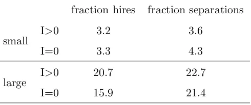
(2010) for a study of interrelated factor demand). Table 1 reports statistics relating

Table 1: Investment and Labor Adjustment

fraction hires fraction separations

small I>0 3.2 3.6

I=0 3.3 4.3

large I>0 20.7 22.7

I=0 15.9 21.4

fraction: Fraction of establishments in %, correlation: Correlation between size of adjustment and size

of investment

relate to annual adjustments. Large establishments are more likely to adjust employment

when they invest. This is particularly true for hires. 20.7% of large establishments have

hired in a year in which they have reported investment, compared to 15.9% of hiring by

establishments which did not invest. However, investing firms have also been slightly

more likely to contract than those firms which did not invest. For small establishments,

hiring does not seem to be effected much by investment, while separations occur more

frequently at establishments with zero investment. These statistics suggest that

invest-ment might have been labor-compleinvest-menting. Furthermore, small establishinvest-ments seem to

have exploited complementarities by fewer separations, while large establishments have

adjusted through hiring. While labor-capital complementarities are present, they seem

to be more important for bigger establishments.

3

Institutional characteristics

A full characterization of the German labor market and labor relations are out of the

scope of this paper, but a general knowledge of institutions governing or influencing

ad-justment costs is helpful. Apart from a relatively high coverage of employees by collective

agreements (in 2009 56% of all employees in West and 38% in East Germany were covered

Germany are important for adjustment costs:

1. Establishments in Germany engage in training youth entering the labor market.

This happens in the framework of the dual system: Besides working and learning

at an establishment, apprentices attend school for one or two days of the week.

Costs are covered by employers, but net costs of training are notoriously difficult

to calculate. Harhoff and Kane (1997) list studies putting the annual costs of

training one apprentice at a range of 5,000$ to 10,000$ in 1990 dollars (see the

same study for a more detailed overview of this training system).

2. At establishments with at least five permanent employees, workers’ councils can

be set up at the initiative of the employees. These councils need to be informed

and consulted for certain decisions, including restructuring of employment and

recruitment, and enjoy certain co-determination rights for procedures related to

dismissals. See Addison et al. (2001) for a lengthier discussion.

3. Employees at establishments with at least five (since 2004 at least ten) permanent

employees are protected by certain provisions of theKundigungsschutzgesetz -

dis-missal protection bill: Roughly, employees can be dismissed only as a consequence

of misconduct or special business situations (drop in sales, organisational changes).

See BMAS (2010).

In general, adjustment is more regulated – and appears to be more costly – for large

es-tablishments, tenured personnel, and high-wage personnel, since compensation/severance

payments are based on these measures.

4

Data

The data are the matched employer-employee panel (LIAB), of the German IAB

cross-sectional and longitudinal coverage. This paper uses longitudinal version 3, with

14 years of observations for some 4,200 establishments. The data are described at length

in Jacobebbinghaus (2008). Here are the basics: The data consist of two sources, the

establishment panel (short: panel), and the employment history (short: history). Once

a year a survey for the establishment panel is conducted, and establishments are asked

to report sales, employment, investments et cetera. This panel is then matched with

administrative data of the German federal employment agency (history). Every new

employee and separation has to be reported by the employer to this agency. Wages are

also reported. The wage data here are known to be more reliable than survey data, since

they are based on the actual payments reported to the agency. Misreporting is unlawful.

Occupations not subject to social security contributions (certain state employees,

doc-tors with private practices, firm-owners et cetera) are not covered by the data, but some

80% of the German employment is. Thus, I know for any given day how many people

are employed in any establishment covered by the LIAB, how much they earned, their

education, and age. The education variable is reported by employers, and reporting it is

not mandatory. As a consequence, it has more missing values and for some observations

exhibits inconsistencies over time. Throughout this paper, I am using the unbalanced

panel.

4.1 Sales

Sales are from the panel and reported as the total amount of sales in the last year.

Establishments which reported budgets instead of sales are excluded, because they are

probably non-profits. Since I am mostly using a shorter time-frame than years (the

reporting frequency of the panel), yearly sales volumes have to be divided to shorter time

periods (months in this example). One way to do it would be to divide equally across all

twelve months, but there would be unrealistic jumps from December to January. Another

possibility would be to check quarterly aggregate sales for different industries and adjust

Figure 2: Annual sales divided to months, even and smooth

squared sales distances from month to month over the choice of monthly sales, restricting

the sum of sales for a year to equal the sales reported by the establishment:

min

{st}T_t=1

J =

T

X

t=2

(st−st−1)2 s.t.

12

X

t=1

= S1

24

X

t=13

= S2

.. .

withS1 the reported sales in the first year, S2 in the second year, and so forth. This is

equivalent to smoothing the jumps between monthly sales. Figure 2 depicts an

estab-lishment with 10 years of data.

The blue, solid line shows the sales data divided evenly across the months of a year,

the dashed red line presents the sales data after the described procedure. I estimated

very similar results, lending some support to the robustness of the results to the choice

of how to divide the reported annual sales to months. The results presented in this paper

are for the smoothed sales series.

4.2 Employment

I estimate adjustment costs for different labor aggregates and for different time

perspec-tives (month, quarter, semester, year). I have aggregate labor, and labor divided into

four categories - old and young, skilled and unskilled. Old workers are workers over 40,

skilled workers are workers with higher education or college-qualifying degrees (at least

12 years of primary and secondary education) together with professional training. Only

full-time workers are considered, and workers with very low (less than 5 Euros daily

wage in January 1993 and inflated by an annual 2.5% thereafter) or high wages (more

than 400 Euros daily wage in January 1993 and inflated by an annual 2.5% thereafter)

are excluded. A problem arises if some type of worker is not employed. First, I do not

observe wages for that type (see next section). Also, the production function becomes

undefined, because of logs of zero and division by zero. Thus, for non-employment, in

the estimation I include dummies for non-employment, and the undefined parts of the

first order conditions are set to zero. Obviously, this problem does not occur if I have

only one type of labor, because the establishments always employ at least one worker.

A hire is recorded if an employee starts working at the establishment and was not

working there the previous day. A separation is recorded if an employee works at an

establishment one day, but not the next. Note that with this definition recalls and

temporary quits will count as adjustment, but immediate contract renewals will not.

4.3 Wages

If an establishment employs at least one worker of a certain typej, I take the median wage

mean, because of some censoring issues with the wage data, but for the whole sample the

mean and median wages are very close for the different types of labor. More serious is the

problem of establishments which have not employed a certain type of labor. Note that this

is not just a non-response or random missing value problem. Since there are many small

establishments in the data, and since net and gross adjustments for small establishments

will overlap much more than for bigger establishments, dropping establishments with

unobserved wages would be undesirable. Furthermore, those establishments have chosen

not to employ, even though they could have done it for some (presumably) observed

wage. It remains to “guess” what that wage was. I take that wage to be the median

wage of that type of labor in the observed state, industry, year, and size category. Here is

an example: A small establishment in the consumer goods manufacturing sector located

in the state of Bavaria has not employed any unskilled, old worker in may 2000. What

was the wage it observed for unskilled, old workers? The median wage of unskilled, old

workers in Bavaria in the consumer goods industry in small establishments in 2000.

4.4 Expectations

Recall the final estimable optimality conditions in the linear cost case in equation (8),

all variables are observed or imputed, except the establishments’ expectations for hiring,

separating, or inactivity for the next period (π+, π−), and the β. I setβ to a number to

make the yearly discounting factor equal to 0.95. For the expectations I pursue the

fol-lowing strategy: I predict the probabilities using an ordered probit model where I regress

adjustment today (the categories being hiring, inactivity, separation) on adjustment last

period, size of adjustment last period, wages last period, sales last period, and a full set

of state and sectoral dummies. The predictions are made separately for small (ten or less

employees) and large establishments. As a robustness check, I create cells of

establish-ments of equal period, size, sector, state, and adjustment, with potentially T*2*14*16*3

cells, where T is the number of time periods. The fraction of establishments in a cell

excluding the establishment to which π+ is being assigned). Put differently, given

ob-servable characteristics of an establishment and its adjustment today, I guess that next

period it will behave like similar establishments which have made the same adjustment

in this period. The latter approach has the advantage of avoiding any distributional

assumptions, but creates a good number of empty or single-element cells. Moreover, the

establishments in the single-element cells are likely to be a non-random sub-sample of all

establishments. The results with this approach did not differ qualitatively, but estimates

were comparable for hiring and distinctly higher for separation costs (by a magnitude of

four).

5

Estimation

Estimation is by GMM and follows the procedure outlined in Arellano and Bond (1991)

– a workhorse in estimating dynamic panel models – with little differences due to

nonlin-earities in this application. Denote establishments by i and rewrite the first-differences

of equations (2) and (8)

∆(pi,tqi,t0 )−∆wi,t−a∆(li,t−li,t−1)−b∆(eb(li,t−li,t−1)) + ∆(εi,t) = 0 (2.2’)

∆(pi,tq0i,t)−∆wi,t+τ−∆(1li,t−1>li,t−βπ

−

i,t)−τ+∆(1li,t>li,t−1−βπ

+

i,t) + ∆(εi,t) = 0 (2.8’)

Letεi,t =µi+δt+ui,t The first difference takes out any establishment-fixed effects. With

a vector of instrumentsZ such thatE(∆u|Z) = 0 the equations above can be estimated

by GMM. The typical assumption to qualify endogenous variables lagged two periods

and more as instruments is no serial correlation in the ui,t. Endogenous variables in

t−2 will be uncorrelated with ui,t and ui,t−1 and valid instruments for ∆(li,t −li,t−1),

∆(1li,t>li,t−1 −βπ

+

i,t) et cetera, and possibly weak instruments for ∆(pi,tq0i,t), since the

second lags do not enter into this last expression. Summarizing, since wages and period

dummies are assumed exogenous, the instrument vector Z for equation (2.2’) consists

of pi,tqi,t0 (levels), of lt, and of e−lt. For (2.8’) Z consists of: Differenced wages and

period dummies, second and third lags of the components of pi,tqi,t0 (levels), second and

third lags of (1li,t−1>li,t−βπ

−

i,t) and (1li,t>li,t−1 −βπ

+

i,t). Where I used different lags for

robustness checks, this is made explicit. Equations (2.2’) and (2.8’) are then estimated

by 2-step GMM usingZ as instruments.

6

Results

The benchmark results are for the asymmetric, linear cost model with monthly

ments. I also discuss results for the convex model and for different frequencies of

adjust-ment. The convex model implies sensible adjustment costs for only a small adjustment

range, and longer than monthly frequencies contradict theoretical predictions.

Table 2 reports results for the model with one type of labor and monthly adjustments.

The first panel lists results using all time periods, but dummies for quarters (due to

computer memory constraints). The second uses quarter dummies for the middle third

of the panel (from September 1997 to April 2002). The third panel covers the same

period but uses monthly dummies. Finally, the fourth panel uses monthly dummies but

only observations from the year 2000, corresponding to the middle of the time covered

by the panel. The reason for comparing these four sets of data is the unusual long

dimension of the panel (166 months) and the uncertainties associated with estimates

and test procedures for long panels. Specification 1 is on the full sample, specification

2 excludes establishments for which gross adjustment is different from net adjustment

(hiring and separations taking place within the month), 3 uses only small establishments

(less than 10 employees), and 4 only big establishments.

All coefficients had the predicted signs (adjustment costs are actually positive).

Hir-ing is costly, at around 4,000 Euros per hire. Note that neither prices nor wages have

been adjusted at any point, so we might think of these as end of 1999 - beginning of 2000

estimate drops for big establishments. I suggested above that for legal and institutional

reasons we should expect higher costs for big establishments, but that aggregation might

bias results downward. Comparing this estimate to the second specification, which

ex-cludes establishments which hire and face separations within the same month, suggests

that aggregation bias for hiring costs is substantial, at over 50%. Third, separations

seem to be very inexpensive. Significant estimates of separation costs range around

1,000 Euros, and often enough the costs are insignificant.1 This might be surprising

at first glance, but mind that every separation is counted, including retirements2 and

voluntary quits, which are both presumably costless or associated with small costs for

the employer. Survey results from the German Micro-census suggest that one fifth to

one fourth of all separations are involuntary on the part of the employee (e.g. firings,

own calculations), so that 4,000 to 5,000 Euros might be a more accurate estimate of

firing costs. Fourth, the over-identification tests in the full samples with close to half a

million observations almost always reject the exogeneity assumption for the instruments,

except for small establishments, very likely due to more homogeneity within this

sub-sample, whereas heteroscedasticity is likely to be an issue for the big establishments and

for the full sample. Going to subsequently smaller samples (panels two to four), the

Sargan test statistics become smaller without changing the cost estimates, and for the

sample covering observations from the year 2000 only, exogeneity is not rejected in any of

the specifications, except weakly for big establishments. What explains this sensitivity of

overidentification tests to the sample size? I suspect that the high number of observations

leads to more type I errors - or the reverse might be true: lower number of observations

result in the test NOT rejecting exogeneity when it should. I circumvent this technical

problem here by checking the robustness of the results to the use of different lags. Using

higher order lags allows for some autocorrelation in the residuals ui,t, but comes at the

expense of becoming less “informative” for the endogenous variables. So far, second and

1

The non-parametric approach of predicting adjustment probabilities estimates separation costs of

2,400 Euros for the full sample.

2

Pensions in Germany are for the most part through a mandatory governmental, pay-as-you-go system.

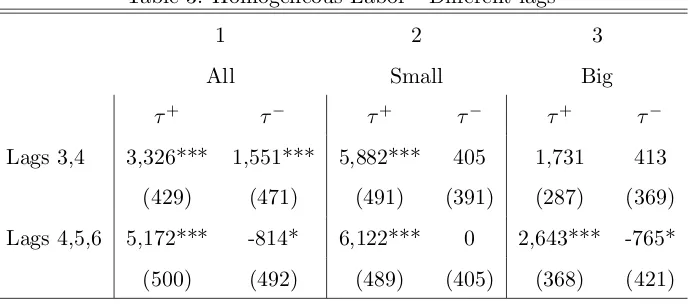
Table 3: Homogeneous Labor - Different lags

1 2 3

All Small Big

τ+ τ− τ+ τ− τ+ τ−

Lags 3,4 3,326*** 1,551*** 5,882*** 405 1,731 413

(429) (471) (491) (391) (287) (369)

Lags 4,5,6 5,172*** -814* 6,122*** 0 2,643*** -765*

(500) (492) (489) (405) (368) (421)

Note: Standard errors in parentheses. P-values:***<0.01, **<0.05, *<0.1

third period lags of endogenous variable levels have been used as instruments.

Table 3 reports estimates for two different sets of instruments. The upper panel uses

the third and fourth lags, and the lower panel the fourth to sixth lags of the endogenous

variables. The use of lags 3 and 4 gives results in the ballpark of the previous estimation.

With lags 4, 5, and 6 estimated hiring costs increase somewhat, but the results for

separation costs become nonsensical. The instruments will become weaker the further

we go back in the lags for the instruments.

Table 4 reports results for different time periods – a comparison for which the data set

is perfectly suited. Flows and stocks of employees are calculated over quarters, semesters,

and years, possibly successively increasing the inaccuracy of measured adjustment.

We see that – except for semesters – in absolute values the coefficients increase for

longer time periods, which is not surprising given that this effectively allows adjustment

costs to be incurred over a longer time interval. Looking at small establishments, hiring

costs seem to increase proportionally to the length of the time interval (by a factor of

five for quarters and semesters, and by a factor of 10 for the year). However, the model

in months is the only one which always yields coefficients in accordance with theoretical

neces-Table 4: Homogeneous Labor - Different time periods

1 2 3

All Small Big

τ+ τ− τ+ τ− τ+ τ−

Monthly 3,745*** 877*** 5,164*** 1,015*** 1,715*** 396***

(224) (202) (491) (391) (287) (110)

Quarterly 14,073*** -2,764*** 25,085*** -2,801*** 8,369*** -2,569***

(1,328) (607) (2,253) (852) (749) (432)

Half-annual 1,585** -869 23,171*** -7,167*** 3,296*** -1,904***

(777) (544) (2,574) (956) (271) (172)

Annual 52,464*** -22,252*** 47,781*** -4,961** -13,276* 6,879*

(15,232) (6,822) (12,898) (2,151) (7,426) (3,782)

Note: Standard errors in parentheses. P-values:***<0.01, **<0.05, *<0.1. Monthly specification

includes quarter dummies. All other specifications include corresponding time dummies.

sarily reject the use of lower than monthly frequencies. One could as well argue that the

model specification is rejected. While this might be true, it would amount to a

concep-tual rejection of the setup of many dynamic labor demand models. Yet, the results are

at odds with papers which have used quarterly and annual data but have not found cost

estimates inconsistent with theoretical predictions, such as Lapatinas (2009), Ejarque

and Portugal (2007), and Cooper et al. (2004). However, these studies impose symmetry

in the variable components and sometimes fixed component of hiring and firing costs. I

have repeated the estimations with different time periods under the constraintτ+=τ−.

The results are reported in table 5. The results obtained under the constraint τ+=τ−

are consistent with our expectation of positive adjustment costs, and the temporal

ag-gregation issue is still apparent. Quarterly adjustment results are somewhat close to

and higher than monthly adjustment results, but going to lower frequency adjustment

results in a dramatic drop of the estimated costs. While this seems to lend more

Table 5: Homogeneous Labor - Different time periods, Symmetric costs

1 2 3

All Small Big

τ τ τ

Monthly 2,345*** 3,062*** 1,178***

(117) (155) (48)

Quarterly 2,833*** 5,304*** 1,465***

(370) (512) (90)

Half-annual 100** 567 129***

(45) (384) (11)

Annual 212*** 492 348

(59) (329) (360)

Note: Standard errors in parentheses. P-values:***<0.01, **<0.05, *<0.1. Monthly specification

includes quarter dummies. All other specifications include corresponding time dummies.

in hiring and separation costs resulted innegative separation costs only when quarterly

adjustment was assumed.

How do the estimates compare with a model of convex costs? Note first, that the

actual behavior of inactivity of most establishments is more consistent with a linear

cost model than with a convex cost specification. Since one model does not nest the

other, formal tests of misspecification can not be performed. However, with comparable

sample sizes, and the same number of parameters and moment conditions, first step

minimized GMM objective function values were higher for the convex model for the full

sample, for small establishments, and for establishments with gross adjustment equaling

net adjustment. Not surprisingly, in this sense the convex model had a worse “fit” than

the linear model. Table 6 reports estimates of the convex model. The first column of

any of the four samples restricts the parameter b in equation (2) to be zero, imposing

Table 6: Homogeneous Labor - convex costs

(1) (2) (3) (4)

All Gross=Net Small Big

a 241** -0.007*** 9*** -0.002*** 382** 29 40** -2.6

(quadratic) (101) (0.001) (3) (0.0004) (165) (38) (19) (4.6)

b -0.002*** 1,730*** 1.3*** -20.9***

(exponential) (0.0001) (77) (0.1) (0)

Note: Standard errors in parentheses. P-values:***<0.01, **<0.05, *<0.1. Regressions include quarter

dummies.

for asymmetry. In the symmetric case, the coefficient is always significantly positive,

as it should be, and we see the familiar pattern that cost estimates are much lower

for big than for small establishments. The coefficient for establishments with gross=net

adjustment is lower in absolute value than the one for big establishments, which is rather

puzzling. The estimates for small (big) establishments imply adjustment costs of 191 (20)

Euros for an adjustment by one, 4775 (500) Euros for an adjustment by five, and 19,100

(2,000) Euros for an adjustment by ten employees. The asymmetric model fails to yield

sensible estimates for big establishments, most likely due to the difficulty of fitting a cost

curve which becomes very steep very fast to a sample with a great degree of size and

adjustment heterogeneity. The coefficients implynegative – if tiny – costs for expanding

the pool of employees. For small establishments the qualitative results from the linear

model are replicated: Hiring is more costly than separations. The estimates imply that

hiring one worker costs 16 Euros, hiring 5 workers costs 204 Euros per hire, and hiring

10 workers costs 44,000 Euros per hire. Going beyond that leads to a rapid explosion

of costs. These numerical examples illustrate a major problem with convex cost models:

The model fits reasonably well for a certain range, but becomes unrealistic for big (and

small) adjustments. Thus, a comparison of results and implied adjustment costs seem to

Figure 3: Size of adjustment if any - all establishments

I turn to the case of heterogeneous labor with linear costs. Unfortunately, the

deriva-tions from section 2 do not go through without further assumpderiva-tions, due to possible

complementarities in different types of labor. The first order condition for the

employ-ment of type j labor becomes:

pt

∂qt

∂lj,t

−wj,t−τ_j+

1lj,t>lj,t−1−βπ

+

j,t

+τ_j−

1lj,t−1>lj,t−βπ

−

j,t

+βX

k6=j

∂lk,t

∂lj,t

π_k,t+τ_k+−π−_k,tτ_k−

= 0

This condition differs from the previous equation in the inclusion of the last summation

(see appendix A for a full derivation). Note that the last term includes the change in the

optimal choice of typeklabor, when the optimal choice of typejlabor changes. For the

estimation I will assume the terms in the summation to be zero, while the cross-terms

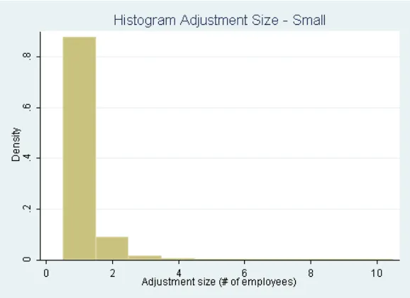
in the production function are preserved. To gauge how restrictive this assumption is I

have plotted histograms for adjustment size conditional on adjustment taking place, cut

– not truncated – at an adjustment size of 11. Figure 3 shows the histogram for all

establishments. It is clear that most adjustment is of only one employee. Adjustments of

two or more employees are not uncommon, but the right tail of the histogram becomes

Figure 4: Size of adjustment if any - small establishments

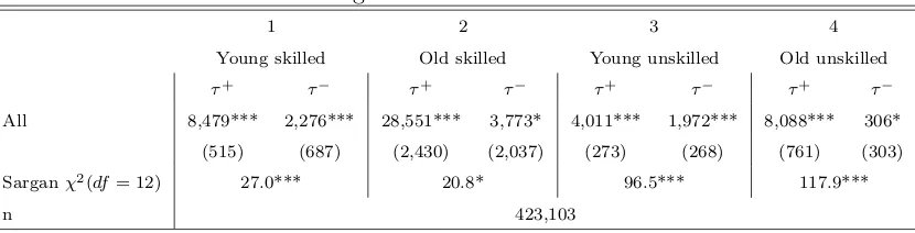
Building on this, table 7 reports results for heterogeneous labor. We would expect

skilled labor to be more expensive to adjust, and the estimation results confirm this.

Hiring skilled, young workers is twice as costly as hiring unskilled ones, and the difference

between old skilled and unskilled workers is even stronger. Indeed, hiring skilled and old

workers seems quite expensive, at more than 28,000 Euros. Separations, too, are more

costly for skilled workers. The high test statistics for the over-identification tests are

discomforting, but the possible roles of large sample sizes and establishment heterogeneity

have been discussed. I have run the same estimation by sectors (not reported). In only

2 of 51 cases is the exogeneity of the instruments rejected, while the general pattern of

hiring and separation costs is confirmed.

7

Conclusion

What has been learned from this exercise? The old news is: First, adjustment costs are

present, and second, convex cost models provide sensible approximations only for small

Table 7: Heterogeneous labor - All establishments

1 2 3 4

Young skilled Old skilled Young unskilled Old unskilled

τ+ _τ− _τ+ _τ− _τ+ _τ− _τ+ _τ−

All 8,479*** 2,276*** 28,551*** 3,773* 4,011*** 1,972*** 8,088*** 306*

(515) (687) (2,430) (2,037) (273) (268) (761) (303)

Sarganχ2_{(df= 12) 27.0*** 20.8* 96.5*** 117.9***}

n 423,103

Note: Standard errors in parentheses. P-values:***<0.01, **<0.05, *<0.1 Regressions include a full set of quarter dummies.

Hiring is more costly than separations – but maybe not more than firings or layoffs.

This last point can not be settled given the absence of the reason for separations in the

data. Fourth, aggregation in time and “space” matter a great deal, and this finding is

the major novelty of this paper. Under asymmetric costs, longer time intervals result

in higher estimates of hiring costs, possibly due to capturing a longer actual incidence

of costs, but reject the model predictions for separation costs frequently. If adjustment

costs are assumed to be symmetric, monthly and quarterly adjustment frequencies yield

comparable results, but in comparison annual adjustment cost estimates drop by 90% and

are economically negligible. Costs are always estimated as lower for big establishments,

for which gross changes in employment are more likely to differ from net changes. Finally,

and reassuringly, in general the model yields higher cost estimates for skilled and for older

labor.

The third result – hiring costs exceeding separation costs – may come as a surprise

and contrasts with findings for Norway by Nilsen et al. (2006). I offer some tentative

explanations: As mentioned earlier, voluntary separations on the side of the employee

may be costless or cheap for the employer. Only a fraction of all separations are

involun-tary to the employee (20%-25% according to own estimates from Micro-census data). A

more subtle explanation might be the treatment of costs as coefficients. Employers have

some, maybe a lot of discretion on how much to invest into searching new employees,

who turns out to be a bad match. Employers might then invest in search, to minimize

involuntary separations. As a result, hiring is costly and separations are not, because

they happen voluntarily most of the time (as matches should be good as a consequence

of costly search).

The work here could be extended in several ways to deepen our understanding of

the working and consequences of adjustment costs. Hiring costs could be endogenized in

a search-framework and welfare analyzes based on the costs and benefits – in terms of

unemployment and risk-reduction – are possible extensions.

References

[1] Abowd, John M. and Francis Kramarz (2003), “The Costs of Hiring and

Separa-tions,” Labour Economics, 10, 499-530.

[2] Addison, John T. Claus Schnabel, and Joachim Wagner (2001), “Works Councils in

Germany: Their Effects on Establishment Performance,” Oxford Economic Papers,

53(4), 659-694.

[3] Arellano, Manuel, and Stephen Bond (1991), “Some Tests of Specification for Panel

Data: Monte Carlo Evidence and an Application to Employment Equations,”

Re-view of Economic Studies, 58(2), 277-297.

[4] Asphjell, Magne K. , W. Letterie, Øivind A. Nilsen, and Gerard A. Pfann (2010),

“Sequentiality versus Simultaneity: Interrelated Factor Demand,” Working Paper.

[5] Berndt, Ernst R. and Laurits R. Christensen (1973), “The Translog Function and

the Substitution of Equipment, Structures, and Labor in U.S. Manufacturing

1929-68,” Journal of Econometrics, 1(1), 81-113.

[6] BMAS (2010), Federal Ministry of Labor and Social Issues booklet, available under

[7] Caballero, Ricardo J. Eduardo M.R.A. Engel, and John C. Haltiwanger (1997),

“Ag-gregate Employment Dynamics: Building from Microeconomic Evidence,” American

Economic Review, 87(1), 115-137.

[8] Cooper, Russell W. John C. Haltiwanger, and Jonathan Willis (2004), “Dynamics

of Labor Demand: Evidence from Plant-level Observations and Aggregate

Implica-tions,” NBER Working Paper 10297.

[9] Ejarque, Jo˜ao M. , and Pedro Portugal (2007), “Labor Adjustment Costs in a Panel

of Establishments: A Structural Approach,” IZA Discussion Paper 3091.

[10] Hall, Robert E. (2004), “Measuring Factor Adjustment Costs,” Quarterly Journal

of Economics, 119(3), 899-927.

[11] Hamermesh, Daniel S. (1989), “Labor Demand and the Structure of Adjustment

Costs,” American Economic Review, 79(4), 674-689.

[12] Hamermesh, Daniel S. (1992), “A General Model of Dynamic Labor Demand,”

Review of Economics and Statistics, 74(4), 733-737.

[13] Hamermesh, Daniel S. (1993) “Spatial and Temporal Aggregation in the Dynamics

of Labor Demand,” in J.van Ours, G.Pfann and G.Ridder, eds. Labor Demand and

Equilibrium Wage Formation, North-Holland.

[14] Hamermesh, Daniel S. and Gerard A. Pfann (1996), “Adjustment Costs in Factor

Demand,” Journal of Economic Literature, 34(3), 1264-1292.

[15] Harhoff, Dietmar, and Thomas J. Kane (1997), “Is the German Apprenticeship

System a Panacea for the U.S. Labor Market?” Journal of Population Economics,

10(2), 171-196.

[16] IAB (2010), IAB-Info from March 2010.

[18] Lapatinas, Athanasios (2009), “Labour Adjustment Costs: Estimation of a Dynamic

Discrete Choice Model Using Panel Data or Greek Manufacturing Firms,” Labour

Economics, 16, 521-533.

[19] Nilsen, Øivind A. Kjell G. Salvanes, and Fabio Schiantarelli (2007), “Employment

Changes, the Structure of Adjustment Costs, and Plant Size,” European Economic

Review, 51, 577-598.

[20] Varej˜ao, Jos´e, and Pedro Portugal (2007), “Employment Dynamics and the

Struc-ture of Labor Adjustment Costs,” Journal of Labor Economics, 25(1), 137-165.

A

Demand for heterogeneous labor

Take equation (3) and extend it toK types of labor.

V(lt−1,It) = max lt

ptq(lt)−wt·lt−

X

k

τ_k+1lk,t>lk,t−1(lk,t−lk,t−1)

−X

k

τ_k−1lk,t−1>lk,t(lk,t−1−lk,t) +βEV(lt,It+1)

Setting up a Lagrangian with constraints lk,t ≥lk,t−1 for all k, we get the following first

order conditions:

pt

∂q

∂l1 −w1,t−τ +

1 +λ+1,t+βE

∂V(lt,It+1)

∂l1,t

= 0

.. .

pt

∂q ∂lK

−wK,t−τ_K++λ+_K,t+βE

∂V(lt,It+1)

∂lK,t

= 0

This needs to be done for all hiring and separation combinations. Similarly, the

ex-pressionE_∂l∂V k,t

can be split into the sum of all different hiring-separation combinations

type of labor next period, the last term of the first order condition for labor type j in

this period would be

∂V(lt,It+1)

∂lj,t

= pt+1

X

k

∂q ∂lk,t+1

∂lk,t+1 ∂lj,t

!

−X

k

wk,t+1 ∂lk,t+1

∂lj,t

−X

k

τ_k+

∂lk,t+1 ∂lj,t

− ∂lk,t

∂lj,t

Collecting all terms ∂lk,t+1

lj,t and using envelope theorems, we and up with

∂V(lt,It+1)

∂lj,t

=X

k

τ_k+

∂lk,t

∂lj,t

Do this for all possible hiring-separation combinations, multiply them by the

correspond-ing probabilities to getE

∂V ∂lj,t

, and plug this back into the first-order conditions, which