A Maximum Eigenvalue Approximation for Crack-Sizing Using Ultrasonic Arrays

A Maximum Eigenvalue Approximation for Crack

Sizing using Ultrasonic Arrays

Laura Cunningham

, Anthony J. Mulholland

, Katherine M. M.

Tant

, Anthony Gachagan

, Gerry Harvey

, and Colin Bird

1

_{Department of Mathematics and Statistics, University of}

Strathclyde, Glasgow, U.K.,G1 1XH

2

_{Centre for Ultrasonic Engineering, University of Strathclyde,}

Glasgow, U.K.,G1 1XW

3

_{PZFlex Europe, 50 Richmond Street, Glasgow, UK, G1 1XP}

4

_{Doosan Babcock, T&E Building, Porterfield Road,}

Renfrew,Glasgow, UK, PA4 8DJ

May 20, 2015

Abstract

Ultrasonic phased array systems are becoming increasingly popular as

tools for the inspection of safety-critical structures within the non-destructive

testing industry. The datasets captured by these arrays can be used to image

and nature of any defects to be deduced. Unfortunately, many of the

cur-rent imaging algorithms require an arbitrary threshold at which the defect

measurements can be taken and this aspect of subjectivity can lead to

vary-ing characterisations of a flaw between different operators. This paper puts

forward an objective approach based on the Kirchoff scattering model and

the approximation of the resulting scattering matrices by Toeplitz matrices.

A mathematical expression relating the crack size to the maximum

eigen-value of the associated scattering matrix is thus derived. The formula is

analysed numerically to assess its sensitivity to the system parameters and

it is shown that the method is most effective for sizing defects that are

com-mensurate with the wavelength of the ultrasonic wave (or just smaller than).

The method is applied to simulated FMC data arising from finite element

calculations where the crack length to wavelength ratios range between 0.6

and 1.8. The recovered objective crack size exhibits an error of 12%.

1

Introduction

Non-destructive evaluation (NDE) is the name given to the group of

tech-niques employed to inspect safety critical structures non-invasively. Such

structures include oil rigs, nuclear power stations and aircraft [1]. The

de-velopment of NDE is essential as the detection and characterisation of flaws

in such structures can prevent catastrophic failure. Additionally, it is a

cost-effective approach as components need only be replaced when a defect

occurs within them. Some common NDE technologies include industrial

radiography [2], electromagnetic testing [3], laser inspection [4], liquid

pene-trant testing and ultrasonic testing [5]. Ultrasonic testing is the most widely

applicable of these techniques as it is comparatively inexpensive, portable

Piezoelectric transducers [7] are the most widely used and contain an

ac-tive piezoelectric element which converts the electrical pulse generated into

mechanical energy (and vice versa). The elastic wave is emitted from the

transducer and travels through the component under inspection. The wave

is then reflected and scattered from any obstacles within the component and

received by the transducer. In recent years there has been an increase in the

use of ultrasonic arrays for NDE inspections [8, 9]. An ultrasonic array is

a single transducer that is comprised of a number of piezoelectric elements

(typically between 64 and 256), where each element acts as both a

transmit-ter and a receiver. There are several advantages of arrays to conventional

ultrasonic probes (a device which contains only a single element); they cover

a larger inspection area thus reducing the time taken to conduct an

inspec-tion and they can be used to produce a range of ultrasonic fields such as

plane, focused and steered beams. The full set of time domain transmitted

and received signals recorded by an ultrasonic array is referred to as the

Full Matrix Capture (FMC) data. This is a three dimensional (transmitting

element, receiving element and time) data block and is generated by firing

an ultrasonic wave through one element and then receiving the reflected

signal across the entire array. This process is repeated for each element

until the entire set of signals is recorded to form the FMC dataset. Once

the FMC data has been collected, post processing algorithms are applied

to extract information associated with a flaw; this is the inverse problem.

Considerable effort has been expended in developing techniques to

charac-terise internal defects via the exploitation of these FMC datasets [10–23].

In particular there has been a series of papers developing the Total Focusing

method (TFM) [10–16]. This method uses the time domain signals from the

FMC dataset to systematically focus at each point in the imaging domain,

subjec-tivity is introduced using such empirical imaging techniques as they rely on

arbitraily chosen imaging thresholds at which the defect measurements are

taken. Previous work has been carried out to address this issue in [24–26],

where objective crack length measurements were made using time-frequency

domain scattering matrices. In this paper, an objective model based method

is presented for tackling the specific problem of sizing cracks within an elastic

solid. This method utilises the Kirchhoff scattering model, a high frequency

approximation to the scattering of a linear elastic wave from an ellipsoid

within a homogeneous medium. By approximating the model scattering

matrices by Toeplitz matrices, an expression relating the crack size to the

maximum eigenvalue of the associated scattering matrix is derived. The

formula is analysed numerically to assess its sensitivity to the system

pa-rameters and is finally applied to simulated FMC data arising from finite

element calculations.

2

Kirchoff model and scattering matrices

The Kirchhoff model is used to provide a high frequency approximation

to the scattering of a linear elastic wave from a crack in a homogeneous

medium. The signals scattered from a crack in the host material are

repre-sented in the frequency domain by scattering matrices, which are a function

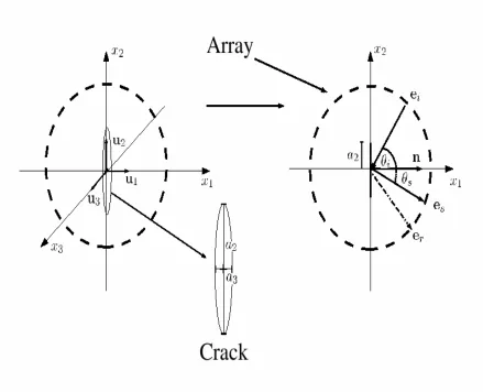
of the transmitted and received waves. Figure 1 shows a schematic of the

model geometry, where the ellipsoidal crack is lying in the plane x1 = 0

and the ultrasonic waves emanating from the array lie in the plane x3 = 0.

An analytical form for the scattering amplitude can be derived by assuming

that the flaw is an ellipsoid (with axes lengths a1, a2 and a3 as in Figure

1). To simulate a zero volume flaw (a crack) in the x3 = 0 plane then the

centre lies at the origin. An expression for the scattering amplitude of an

ellipsoidal crack by a transmitted pressure wave in a homogeneous elastic

medium is then given by (equation (10.168), [27])

An(ei,es) =−

ia2a3eslesnesjCkplj(eip−erp)nk

2ρc2_|e

i−es|re

J1 ³_2π

λ|ei−es|re

´

(1)

whereei andes are the unit vectors in the transmitting and receiving

direc-tion of the ultrasonic wave. It is important to note that in this paper only

pressure waves are considered. The unit vectorer is in the direction of the

specular reflection from the crack; the specular reflection is in the direction

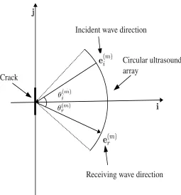
of the maximum amplitude reflected wave. The angle between the specular

reflection direction and the normal to the crack is equal to that between

the direction of the transmitted wave and the normal, as demonstrated in

Figure 2. In addition, c is the wave speed for a pressure wave, ρ is the host material density,λis the wavelength of the transmitted pressure wave,

Ckplj is the elastic modulus tensor, J1 is the Bessel function of the first

kind of order 1 and re is the effective radius of the crack. In an isotropic,

homogeneous medium the elastic modulus tensor in equation (1) reduces to

Ckplj =Lδkpδlj+µ(δklδpj+δkjδpl), whereLandµare the Lam´e co-efficients.

Letting eq = (ei−es)/|ei−es| and u2,u3 be unit vectors along the x2, x3

axis respectively, then the effective radius of the crack is defined as

re =

q

a2₂(eq_·u2)2+a2₃(eq·u3)2 =a2|eq·u2| (2)

sinceei andesare perpendicular tou3. By substituting the definition of the

Figure 1: A schematic of the geometry used to derive the scattering matrices that arise in the Kirchhoff model (equation (1)) for a crack inclusion in an elastic solid. Here 2a2 is the crack length, n is the

normal to the crack, ei (er,es) is the transmitted (receiving, specular)

wave direction, θi(θs) is the angle measured in an anticlockwise

direc-tion from the positive x1 axis of the transmitted (received) wave and

u1,u2 and u3 are unit vectors in the x1, x2 and x3 directions.

that

An(ei;es) =−

ia3esn(L((ei−er)·n) + 2µ((ei−er)·es)(es·n))

2ρc2_|(e

i−es)·u2|

J1 ³_2πa2

λ |(ei−es)·u2|

´

.

(3)

where the scale factor a3 has been dropped and the scattering amplitude

Incident wave direction

Receiving wave direction

Crack

Circular ultrasound

array

Figure 2: A schematic showing the location of the unit vector in the specular reflection direction, e(rm), with respect to the unit vector in

the incident direction, e(_im), on a limited aperture, circular array.

the direction of reception,es. The transmitted and received wave directions

can be defined at a discrete set of values and if these completely surround

the flaw it is called a full aperture. By calculating the absolute value of

the scattering amplitude given in equation (3) for every possible pair of

transmitting and receiving angles (at a fixed frequency), a scattering matrix

can be constructed, with the largest entries occuring close to the specular

3

Approximation to a limited aperture

ul-trasonic array

The Kirchhoff model provides the response from a full aperture, circular

array which is shown by the dashed line in Figure 1. However, in this work

the circular array is approximated by a discretised linear limited aperture

array as this is all that can be measured in practice. The approximation

to a limited aperture array allows the expression for the scattering matrices

given by equation (3) to be parameterised. The unit vector in the receiving

direction for thenth element in the ultrasound array is given by

e(_sn)= p d

d2_+q2

n

i+ p qn

d2_+q2

n

j=p1₋qˆ2

ni+ ˆqnj. (4)

wheredis the minimum distance between the flaw and the ultrasound array (it is assumed here that the centre of the array is the closest point in the

array to the flaw),qn dictates the element position,

qn= △

q

2 (N + 1−2n), (5)

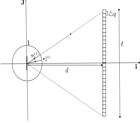
where N is the total number of elements in the ultrasound array and the periodicity of the array elements (the pitch) is given by

△q = l

N₋1 (6)

wherel is the array length (aperture) as shown in Figure 3.

Figure 3: A schematic demonstrating the geometry of the linear ultra-sound array. The unit vectore(sn) is in the receiving direction for array

elementn on the array. The array is of length l, the flaw is at a depth

d from the array and_△q gives the pitch between the array elements. ofn. Combining equations (4), (5) and (6) then

ˆ

qn=

l

p

4d2_+l2_(1−h(n))2

N+ 1₋2n

N₋1 (7)

in equation (7) is manipulated further to give

ˆ

qn=

l

√

4d2_+l2

N + 1₋2n N ₋1

1

√

1₋α (8)

where α = l2(2h₋h2)/(4d2 +l2). Since 0 _≤ h _≤ 2 for n = 1, ..., N then 0_≤2h₋h2_{≤1, and since 0< l}2_/(4d2_+l2_{)<1, then α is small. A Taylor}

series approximation is applied to equation (8) to approximate ˆqn as

ˆ

qn=yn+O(α2) (9)

where

yn=△y(N + 1−2n)/2 (10)

and

△y= l

((N ₋1)√4d2_+l2₎. (11)

From equation (4) the approximate transmitting and receiving unit vectors

are therefore given by

e(_im)=₋p1₋y2

mi−ymj, m= 1, ..., N (12)

and

e(_sn)=p1₋y2

ni+ynj, n= 1, ..., N. (13)

By restricting attention to the case where the flaw is orientated to lie along

thex2 axis then the specular reflection is given by

e(_rm) =p1₋y2

mi−ymj, m= 1, ..., N (14)

becomes

A(ym, yn) =

p

1₋y2

m

ρc2_|y

n+ym|

(L+2µ(1₋y_n2))J1 ³

2πˆa_|yn+ym|

´ _.

= 1

ρc2Am,n (15)

where ˆa = a2/λ and 2a2 is the crack length. In the next section a crack

sizing method is developed which relates the maximum eigenvalue of the

scattering matrixAm,n to the length of the crack.

4

Crack sizing using the maximum

eigen-value

It is clear from empirical observations that there is a relationship between

the size of the crack and the form of the scattering matrix [25]. It would

therefore be advantageous if an analytical approach could be developed to

capture this correlation. From the scattering matrices in Figure 4 it can be

seen that the dominant values aggregate around the skew diagonal. There

is a considerable body of research concerning Toeplitz matrices and in an

effort to benefit from this body of work the scattering matrix,A (given by equation (15)), will be approximated by a Toeplitz matrix. First, the matrix

Ais transformed toAT via

AT(ym′, y_n) =A(y_m, y_n) where m′ =N −m+ 1 (16)

so that the dominant values accumulate around the main diagonal. The

transformed scattering matrix,AT, will be approximated by a Toeplitz

ma-trix, where the row where the maximum of AT(ym, yn) occurs will be used

to create this Toeplitz approximation, ¯AT. This row is highlighted by the

the transformed matrix,AT, in Figure 4 (b). The Toeplitz matrix resulting

from this matrix is shown in Figure 4 (c) where all remaining entries in the

row are filled with zeroes. To begin we observe that in equation (15) the

term

J1(2πˆa(yn+ym))

yn+ym

(17)

obtains its maximum whenyn+ym= 0.The prefactor to the Bessel function

in equation (15) is given by

p

1₋y2

m(L+ 2µ(1−y2n′)), (18)

and, since 0 < y2_m, y2_n < 1, this is also maximised when ym = yn = 0.

Since the array is centred on the x1-axis, this means that ym = yn = 0

corresponds to the centre of the array. IfN is odd then the central element is given by n=m = (N + 1)/2 and if N is even then the smallest value is

ym =yn =−△y/2 which occurs at n=m =N/2 + 1. In what follows the

focus will be on the case whereN is even (the analysis is virtually identical for the case whereN is odd) and so we will take this row of A (and hence

AT) to form our Toeplitz approximation. Substituting ym = −△y/2 into

equation (15) gives the first N/2 entries in the first row of the Toeplitz matrix ¯AT as

¯

AT(yp) =

2p1_{− △}y2_{/4(L+ 2µ(1−y}2

p))

ρc2_(2y

p− △y)

J1 ³

2πˆa

µ

yp−△

y

2

¶´

(19)

wherep=N/2 + 1, ..., N and the absolute value has been removed asyp− △y/2 < 0 and J1(2πˆa(yp − △y/2)) < 0. This row is highlighted in the

scattering matrix shown in Figure 4 (b). The remaining terms in the first

row of ¯AT are set equal to zero (that is ( ¯AT)j = 0, j =N/2 + 1, ..., N). The

n=1 n=N

m=N n=1 m=1

m=n=N/2+1

n=N n=1

m'=N m'=1

m'=N/2, n=N/2+1

(a) (b)

(c)

Figure 4: The original scattering matrix,A (equation (15), is shown in (a) where the green squares highlight the section of the row which is used to construct the Toeplitz approximation. This is the row where the maximum occurs at n = m = N/2 + 1. The red dashed lines highlight the rows which are shown to be approximately equal to the portion of the row where the maximum occurs (shown by the green squares). The equivalent is highlighted in the transformed matrix, AT

(equation (16)), in (b) and (c) shows the Toeplitz matrix, ¯AT (equation

by showing that

¯ ¯ ¯ ¯

A(y_N/2+1, yn)−A(ym, yn−m+N/2+1)

A(y_N/2+1, yn)

¯ ¯ ¯

¯=O(ǫ) ∀m, n=N/2 + 1, ..., N,

(20)

where 0< ǫ_≪1 is of the order of the array aperture size squared (typically

ǫ_{∼ O}(10−2_{)) (see Appendix A).}

4.1

An approximation for the maximum eigenvalue

of the Toeplitz form of the scattering matrix.

In the forthcoming section an approximation which relates the radius of a

crack in terms of the wavelength, ˆa, to the maximum eigenvalue σmax of

the Toeplitz approximation to the scattering matrix will be derived. This

maximum eigenvalue is approximated using an upper bound, σB, which is

given by [28]

σB= ( ¯AT)1·w (21)

where ( ¯AT)1 = (( ¯AT)1,1,|( ¯AT)1,2|, ...,|( ¯AT)1,N|), w= (1, w2, ...wN) and

wk(N) = 2 cos

Ã

π

¥_N−1

k−1

¦

+ 2

!

, (22)

where_⌊._⌋ denotes the floor function. The first row of the Toeplitz matrix, ¯

AT(yp), is given by equation (19) and when substituted into equation (21)

gives

σB = ¯AT(yN/2+1) +

N

X

t=N/2+2

|AT(yt)|wt

= ¯AT(yN/2+1) +

N

X

t=N/2+2

Ft(ˆa)

J1(2πˆa(yt− △y/2))

2πaˆ(yt− △y/2)

where

wt(N) = 2 cos

Ã

π

¥2(N−1) 2t−2−N

¦

+ 2

!

, (24)

withk=t₋N/2 and the prefactor is given by

Ft(ˆa) =

2πˆap1₋(_△y)2_/4

ρc2 (L+ 2µ(1−y 2

t)). (25)

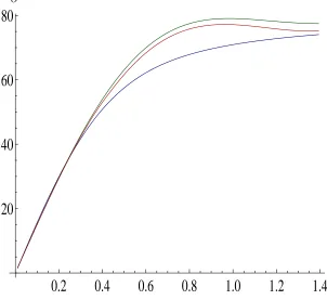
The true (numerically calculated) maximum eigenvalue from a scattering

matrix from the Kirchhoff model is plotted as a function of the crack radius

over the wavelength (ˆa) in Figure 5 (blue line). The approximation to this maximum eigenvalue given by equation (23) is also plotted in this figure

(green line) and there is good agreement as ˆais varied. In order to view the explicit dependency of σB on ˆa it is necessary to make approximations to

the expression within the summation in equation (23). The Bessel function

within equation (23) is approximated by

J1(2πˆa(yt− △y/2))

2πˆa(yt− △y/2)

=       

f_t(1)(ˆa) ifN/2 + 2_≤t_≤t∗

f_t(2)(ˆa) ift∗_{+ 1≤t≤N}

where the approximation for small arguments [29] is used to obtain

f_t(1)(t,ˆa) =

¯

ft(1)

z }| {

1 2

Ã

1₋1 4

µ

πˆa

µ

yt−△

y 2 ¶¶2! +_O à 1 384 µ

πˆa

µ

yt−△

y

2

¶¶4!

(26)

and for large arguments [29]

f_t(2)(t,aˆ) =

¯

ft(2)

z }| {

1 2π2

µ

ˆ

a

µ

yt−△y

2

¶¶−3₂

cos³2πaˆ

µ

yt−△y

2

¶

−3₄π´ (27) +_O

Ã

3 24π3sin

µ

ˆ

a

µ

yt− △

y

2

¶

−3₄π

¶ µ

ˆ

a

µ

yt− △

y

2

¶¶−5₂!

The indext∗ _{determines when the argument of the Bessel function converts}

from small values to large values. An expression for t∗ _{can be determined}

(see Appendix B) and is given in terms of the system parameters and ˆa. Evaluating equation (19) at p=N/2 + 1 gives

¯

AT(yN/2+1) = ¯AT

µ

−△₂y

¶

=FN/2+1(ˆa) =

2ˆaπp1₋(_△y)2_/4¡_{L+ 2µ}¡_1−(△y)2_/4¢¢

ρc2

(28)

where 0 < _△y _≪ 1. The approximation to equation (23) is split into two summations and is therefore given by

σB =FN/2+1(ˆa) +

t∗

X

t=N/2+1

Ft(ˆa)ft(1)¯ (ˆa)wt(N) + N

X

t=t∗₊₁

Ft(ˆa)ft¯(2)(ˆa)wt(N)

+_O(max_{e1, e2}) (29)

where

e1 =

π4_ˆa4

384

t∗

X

t=N/2+1 µ

yt− △

y

2

¶4

wt(N)Ft(ˆa) (30)

and

e2 = 3

24π3

N

X

t=t∗₊₁

µ

ˆ

a

µ

yt−△y

2

¶¶−5₂

sin³2πaˆ

µ

yt−△y

2

¶

−3₄π´Ft(ˆa)wt(N).

(31)

As these error functions are monotonically increasing in t then, by taking

t = t∗ _{for all t upper bounds can be derived (see Appendix B). Further}

approximations are applied to equation (27) to allow σB to be expressed

in terms of a polynomial in t. This will be useful later where the aim is to extract the parameter ˆa in order to obtain an explicit expression which relates σB to ˆa. Let

¯

where

s(1)_t (t,ˆa) = 1

π2

³ ₂

ˆ

a_△y(N ₋2t)

´3₂

, (33)

and

s(2)_t (ˆa) = cos³πˆa_△y(N ₋2t)₋ 3π 4

´

. (34)

The Taylor series approximation ofs1 around the pointt=m= (t∗+N)/2

(the midpoint betweent∗ _{and N) is given by}

s(1)_t (ˆa, m) =

¯

s(1)t

z }| {

1 2π2

µ

1 ˆ

a_△y(N ₋2m)

¶3/2µ

1 + 3

N₋2m(t−m)

¶

+_O

Ã

15ˆa2(_△y)2

µ

1 ˆ

a_△y(N ₋2m)

¶7/2

(t₋m)2

!

. (35) and similarly

s(2)_t (ˆa, m) = cos³πˆa_△y(N₋2t)₋3π 4

´Ã

1₋2³ˆaπ_△y(t₋m)´2

!

+ sin³πˆa_△y(N ₋2t)₋3π 4

´Ã

−2ˆaπ_△y(t₋m) + 4 3

³

ˆ

aπ_△y(t₋m)´3

!

+_O

µ

2

3(πaˆ△y)

4_(t

−m)4cos³πˆa_△y(N ₋2t)₋3π 4

´¶

= ¯s(2)_t +_O

µ

2

3(πˆa△y)

4

(t₋m)4cos³πˆa_△y(N ₋2t)₋ 3π 4

´¶

.

(36)

This gives the approximation

¯

where

e3=O Ã

¯

s(2)_t (ˆa, m)Ft(ˆa)wt(N)15ˆa2(△y)2

µ

1 ˆ

a_△y(N ₋2m)

¶7/2

(t₋m)2

!

(38)

and

e4 =O µ

¯

s(1)_t (ˆa, m)Ft(ˆa)wt(N)

2

3(πˆa△y)

4_(t

−m)4cos³πaˆ_△y(N ₋2t)₋ 3π 4

´¶

.

(39)

Substituting equations (35) and (36) into equation (29) gives

σB=FN/2+1(ˆa) +

t∗

X

t=p+1 h

Ft(ˆa) ¯ft(1)wt(N)

i

+

N

X

t=t∗

h

Ft(ˆa)¯s(1)t (t,a, mˆ )¯s

(2)

t (t,ˆa, m)wt(N)

i

+_O(max_{e1, e2, e3, e4}).

(40)

Finally, wt given by equation (24) is approximated by a linear function.

First the floor function within the cosine in equation (22) is dropped (a

justification is given in Appendix C) to give

wt= 2 cos

Ã

π

2(N−1) 2t−N−2+ 2

!

= 2 cos

µ

π(2t₋2₋N) 2(2t₋3)

¶

The function is then approximated by a Taylor series about 3N/4 (the mid-point in the ranget=N/2 + 1 to t=N) to give

wt(N) =

¯

wt(N)

z }| {

2 cos

µ

π(N₋4) 6(N₋2)

¶

−8π(N₉₍−_N1) (t−3N/4)

−2)2 sin

µ

π(N₋4) 6(N₋2)

¶

+_O

Ã

2

µ

t₋3N

4

¶2µ

8π(N ₋1) 27(N₋2)3

¶ Ã

2 sin

µ

π(N₋4) 6(N₋2)

¶

−π

2_{(N −1)}

3(N ₋2) cos

µ

π(N ₋4) 6(N ₋2)

¶!!

. (42)

This is substituted into equation (40) to give

σB =FN/2+1(ˆa)

+

t∗

X

t=N/2+2

Ft(ˆa) ¯ft(1)w¯t(N)

+

N

X

t=t∗

Ft(ˆa)¯s(1)t (ˆa, m)¯s

(2)

t (ˆa, m) ¯wt(N)

+_O(max_{e1, e2, e3, e4, e5, e6}) (43)

where

e5=O Ã

2

µ

t₋3N

4

¶2µ

8π(N₋1) 27(N ₋2)3

¶ Ã

2 sin

µ

π(N ₋4) 6(N ₋2)

¶

−π

2_{(N −1)}

3(N₋2) cos

µ

π(N₋4) 6(N ₋2)

¶!

×s¯(1)_t (ˆa, m)Ft(ˆa)¯s(2)t (ˆa, m)(N−t)

!

and

e6=O Ã

2

µ

t₋3N

4

¶2µ

8π(N₋1) 27(N ₋2)3

¶ Ã

2 sin

µ

π(N ₋4) 6(N ₋2)

¶

−π

2_{(N −1)}

3(N₋2) cos

µ

π(N₋4) 6(N ₋2)

¶!

×f¯_t(1)(ˆa)Ft(ˆa)(t−N/2)

!

(45)

The expressions within each summation are polynomials in t which allows

σB to be expressed in the following form

σB= ˆAˆa+

6 X

l=1

S_l(1)(ˆa)bl(ˆa) +

8 X

l=1

S_l(2)(ˆa)dl(ˆa) (46)

where

ˆ

A= π

p

1_{− △}y2_{/4)(L+ 2µ}¡_{1− △y}2_/4¢₎

ρc2 , (47)

S_l(1)(ˆa) =

t∗

X

t=N/2+2

tl−1, S_l(2)(ˆa) =

N

X

t=t∗₊₁

tl−1, (48) and bl and dl are functions of ˆa. Since t∗ is a function of ˆa then to derive

an equation where the dependency on ˆais explicit, it is necessary to rewrite these summations so thatt∗ _{does not appear as a limit. Using a closed form}

expression for the sum ton terms oftp [30] then

S_l(1)(ˆa) =(t

∗_{+ 1)}l

l +

l

X

k=1

Bk

l₋k

µ

l₋1

k

¶

(t∗_{+ 1)}l−k₋(N/2 + 2) l l − l X k=1 Bk

l₋k

µ

l₋1

k

¶ µ

N

2 + 2

¶l−k

and

S_l(2)(ˆa) = (N + 1)

l

l +

l

X

k=1

Bk

l₋k

µ

l₋1

k

¶

(N + 1)l−k₋(t∗+ 1) l

l

− l

X

k=1

Bk

l₋k

µ

l₋1

k

¶

(t∗_{+ 1)}l−k ₍₅₀₎

where Bk is thekth Bernoulli number. The coefficients bl are expressed in

terms of a polynomial function in ˆaas follows

bl(ˆa) =b(1)_l aˆ+b(2)_l ˆa3 (51)

whereb(1)_l and b(2)_l are functions of the number of elements in the array,N,

△y, Lam´e coefficients L and µ, wave speed c and material density ρ. The dependency on ˆais extracted from the first summation in equation (46) to give

6 X

l=1

S_l(1)(ˆa)bl(ˆa) =

6 X

l=1

S_l(1)(ˆa)(b(1)_l ˆa+b(2)_l ˆa3)

= ˆaSˆ1(ˆa) + ˆa3Sˆ2(ˆa) (52)

where

ˆ

S1(ˆa) = 6 X

l=1

S_l(1)(ˆa)b(1)_l and Sˆ2(ˆa) = 6 X

l=1

S_l(1)(ˆa)b(2)_l . (53) The coefficientsdl are extracted from equation (40) and are of the form

dl(ˆa) =B(ˆa)

Ã

((d(0)_l +d(1)_l aˆ+d(2)_l ˆa2+d(3)_l aˆ3+d_l(4)ˆa4) cos(p(ˆa)) +(d(5)_l +d(6)_l aˆ+d(7)_l aˆ2+d(8)_l ˆa3+d_l(9)ˆa4) sin(p(ˆa))

!

where

B(ˆa) =

µ

1

πaˆ_△y(2N₋2t∗₋₃₎

¶5/2

, (55)

and

p(ˆa) = π

4 + ˆaπ△yt

∗_{. (56)}

The second summation in the expression forσB, equation (46), can now be

expressed in the form

8 X

l=1

S_l(2)(ˆa)dl(ˆa) =B

8 X

l=1

S_l(2)(ˆa)³(d(0)_l + ˆad(1)_l + ˆa2d(2)_l + ˆa3d(3)_l + ˆa4d(4)_l ) cos(p(ˆa)) + (d(5)_l + ˆad(6)_l + ˆa2d(7)_l + ˆa3d(8)_l + ˆa4d(9)_l ) sin(p(ˆa))´

= ˆS3(ˆa) cos(p(ˆa)) + ˆS4(ˆa) sin(p(ˆa)) (57)

with

ˆ

S3(ˆa) =B(ˆa)(D0+D1aˆ+D2ˆa2+D3aˆ3+D4ˆa4)

=B(ˆa)

4 X

k=0

Dk(ˆa)ˆak (58)

and

ˆ

S4(ˆa) =B(ˆa)(D5+D6aˆ+D7ˆa2+D8aˆ3+D9ˆa4)

=B(ˆa)

9 X

k=5

Dk(ˆa)ˆak−5 (59)

where

Dj(ˆa) =

8 X

l=1

(57) can then be expressed in the form

8 X

l=1

S_l(2)(ˆa)dl(ˆa) =Q(ˆa) cos(p(ˆa)−φ(ˆa)) (61)

where

φ(ˆa) = tan−1 Ã

ˆ

S4(ˆa)

ˆ

S3(ˆa) !

(62)

and

Q(ˆa) =

q

ˆ

S3(ˆa)2+ ˆS4(ˆa)2. (63)

Finally, the approximation to the maximum eigenvalue,σB, from the

scat-tering matrix,A, defined by equation (15) is

σB(ˆa) = ( ˆA+ ˆS1(ˆa))ˆa+ ˆS2(ˆa)ˆa3+Q(ˆa) cos(p(ˆa)−φ(ˆa))

+_O(max_{e1, e2, e3, e4, e5, e6}) (64)

after equations (52) and (61) are substituted into equation (46). Ift∗ _{> N}

thenσB(ˆa) is further reduced to give

σB(ˆa) = ( ˆA1+ ˆS1(ˆa))ˆa+ ˆS2(ˆa)ˆa3+O(max{e1, e6}) (65)

using only equation (52). The final approximation forσB given by equation

(64) is shown in Figure 5 (red line). This again shows good agreement with

the true (numerically calculated from equation (15)) eigenvalue from the

0.2

0.4

0.6

0.8

1.0

1.2

1.4

20

40

60

80

ˆ

a

σ

Figure 5: The maximum eigenvalue as a function of ˆa from the scatter-ing matrices given by equation (15) (Blue line), the upper bound to the maximum eigenvalue from the Toeplitz approximation to a scattering matrix given by equation (23) (Green line) and the final approximation derived from equation to the maximum eigenvalue given by equation (64) (Red line).

5

The effects of varying the system

pa-rameters on the maximum eigenvalue

In order to assess the robustness of this approximation, a comparison with

the numerically calculated maximum eigenvalue from the original scattering

matrix (given by equation (15)) is made, as the system parameters are

var-ied. In this section each of the system parameters (N, the number of array elements,d, the depth of the flaw, andl, the length of the array) are varied in turn. The effects observed are explained by investigating the changes in

5.1

Varying the depth of the flaw,

d

As the scattered wave propagates through the material it is attenuated and

so, in order to discount this effect, we calculate the scattered field by

mul-tiplying the scattered amplitude (given by equation (15)) by exp(ikrm)/rm

whererm =

p

q2

m+d2andqmis given by equation (5). Sinced≈mthen this

scaling factor can be approximated by 1/√2d. The maximum eigenvalues

0.2

0.4

0.6

0.8

1.0

1.2

20

40

60

80

100

ˆ

a σB, σK

(a)

0.2

0.4

0.6

0.8

1.0

1.2

500

1000

1500

ˆ

a σB, σK

(b)

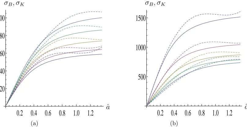
Figure 6: These plots show the approximation to the largest eigenvalue from a scattering matrix,σB (dashed lines), equation (64), and the

nu-merically calculated eigenvalue from the scattering matrix, σK (solid

lines), equation (15), as the crack radius over wavelength, ˆa, is varied (in both cases a prefactor to account for loss of amplitude with depth 1/√2d is used). Each different coloured pair of lines show this com-parison for increasing depths of crack from the array; the flaw depth

d is 30mm (purple), 50mm (red), 70mm (yellow), 90mm (green) and 110mm (blue). The other system parameters are fixed with the number of array elements,N = 64 and the array aperture, l = 128mm.

from the scattering matrices from the approximation,σB, (dashed lines) in

equation (64) and those calculated numerically (solid lines), σK, from the

It can be observed that there is good agreement throughout and that the

values ofσB and σK decrease asdincreases, which is physically intuitive.

5.2

Varying the number of elements,

N

Now the effect of varying the number of elements in the ultrasonic, linear

array on the maximum eigenvalue is examined. In this subsection the other

system parameters are fixed withd= 50mm andl= 128mm. Figure 7 shows the plot of the maximum eigenvalue from the approximationσB, equation

(64), (dashed line) and the mnumerically calculated maximum eigenvalue

from the scattering matricesσK (solid line) as ˆais varied forN= 32 (blue),

64 (red), 128 (yellow) and 256 (green) array elements. This figure shows

0.2

0.4

0.6

0.8

1.0

1.2

50

100

150

200

250

300

ˆ

a σB, σK

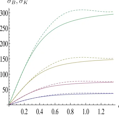
Figure 7: These plots demonstrate the effect of varying the number of elements, N, on the maximum eigenvalue, σB. The approximation

to the largest eigenvalue (dashed lines), equation (64), and the numer-ically calculated eigenvalue from the scattering matrix (solid lines), equation (15), are plotted in (a) as a function of the crack radius over the wavelength ˆafor various numbers of array elements (N= 32 (blue), 64 (red), 128 (yellow), 256 (green)), withl = 128mm and d= 50mm.

that the maximum eigenvalue from the scattering matrix increases as the

is more sensitive (∂σB/∂aˆ increases) to the size of the crack as the density

of the array elements increases. This is to be expected as the increase in the

number of array elements enables more information to be recorded by the

ultrasonic transducer and therefore a higher volume of detail is contained

within the scattering matrix.

5.3

Varying the array length,

l

Increasing the array length has the same effect as decreasing the depth of

the flaw. That is, the total angle the array makes with the crack (the array

aperture angle) increases as the length of the array increases. As the length

0.2

0.4

0.6

0.8

1.0

1.2

50

100

150

ˆ

a σB, σK

(a)

0.05

0.10

0.15

0.20

0.25

80

100

120

140

l σB

(b)

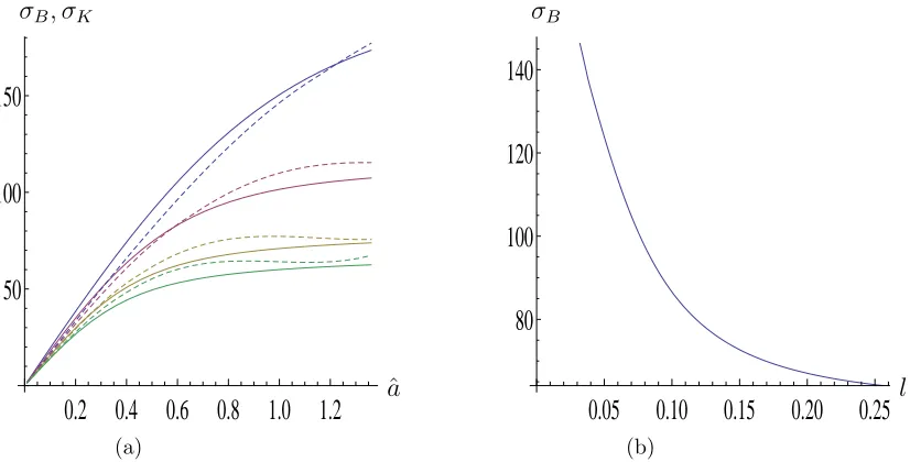
Figure 8: These plots demonstrate the effect of varying the length of the array, l, on the maximum eigenvalue, σB. The approximation to

of the array is increased the maximum eigenvalue,σB (dashed lines), from

equation (64) and the actual maximum eigenvalue,σK (solid lines), decrease

as is shown in Figure 8 where σB and σK are plotted as a function of ˆa

for various lengths of array (l=32mm (blue), 64mm (red), 128mm (yellow) and 256mm (green)). This seems counterintuitive, however, as the array

length is increased (and the array aperture angle is increased) then there

is a larger range of values in the scattering matrix; since more of the main

lobe in the scattering matrix is captured. This in turn leads to broader

spread of eigenvalues and, with less energy being associated with the largest

eigenvalue, its value comes down in magnitude. Note also that here the

number of array elements, N, is fixed and so the information recorded by the ultrasonic transducer is more sparse. In the next subsection the array

length is varied but with the pitch, _△y, fixed and so the number of array elements,N, and the array length,l, increase proportionally.

5.4

Varying the array length,

l

, and the number

of elements,

N

In this subsection the length of the array is varied, however the pitch, _△y

is fixed; this means that the number of elements in the array is a function

of the array length and is given by

N = 2l

△y√4d2_+l2 + 1. (66)

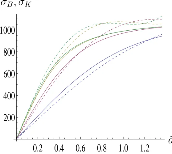
In this section _△y = 0.025 and d = 50mm. Figure 9 shows the approxi-mation to the maximum eigenvalue σB (dashed line) and the numerically

calculated maximum eigenvalue σK (solid line) as ˆa is varied. This figure

shows that the maximum eigenvalue now increases as the length of the array

This suggests that in experimental investigations one should try and retain

a constant pitch when scanning different test peieces (this of course would

naturally occur if one uses the same transducer array probe).

0.2

0.4

0.6

0.8

1.0

1.2

200

400

600

800

1000

ˆ

a

σ

, σ

Figure 9: This plot demonstrates the effect of varying the number of elements, N, and the length of the array l simultaneously on the maximum eigenvalue,σB. The approximation to the largest eigenvalue

(dashed lines), equation (64), and the numerically calculated eigenvalue from the scattering matrix (solid lines), equation (15), are plotted in (a) as a function of the crack radius over the wavelength ˆa for various numbers of array lengths (l= 32mm (blue), 64mm (red), 128mm (yel-low), 256mm (green)), with corresponding N =_{25,44,64,76_} (to the nearest whole number) and the depth of the flaw fixed at d = 50mm. The plot in (b) showsσB asN is varied where ˆa= 1 andd = 50mm.

This investigation into the effects of the system parameters can lead

to other recommendations for experimental designs. For instance, Figure

9 shows that there is very little increase in sensitivity of σB to ˆa when

the array length is increased from 128mm to 256mm (and the number of

elements is increased from 64 to 76 since the pitch is fixed at 2mm here).

a sub-wavelength crack within this medium then it is unnecessary to use

an array larger than 128mm, for a fixed pitch of 2.5mm. The sensitivity

of the maximum eigenvalue to the system parameters can also be studied

analytically by calculating various partial derivatives of the eigenvalue σB

with respect to these parameters (see Appendix D). This work shows that

σB is sensitive in particular to changes in the crack radius to wavelength

ratio ˆa and hence suggests that the inverse problem of recovering ˆa from measured values of the maximum eigenvalue should be viable. Importantly,

the analysis shows that small errors in the length of the array,l, the number of elements,N and the depth of the flaw, ddo not create large errors inσB.

It was also found that σB is particularly sensitive to changes in the crack

radius over the wavelength, ˆa, when ˆa <0.8, which implies that this method should be used for sizing cracks commensurate with the wavelength (or at

least in that neighbourhood) and for ˆa > 0.8 another method, such as an image-based method (TFM for example) should be used.

6

Results from simulated data

In this section the method is applied to simulated FMC data in the time

do-main generated using the finite element package PZFlex [31]. It simulates

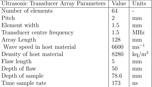
a crack of length 5mm (a = 2.5mm and ˆa _≈ 0.5) within a homogeneous medium, and the parameters used in this simulation are given in Table

1. Each transmit-receive time domain signal was transformed into the

fre-quency domain using a Fast Fourier Transform. A 1.5 MHz single cycle

sinu-soid wave was used in the simulation and so a₋3dBwindow is taken around this central frequency to give a usable bandwidth of 0.75₋2.25MHz (this gives of a range of 0.6 to 1.8 for the crack length to wavelength ratio). The

Ultrasonic Transducer Array Parameters Value Units

Number of elements 64

-Pitch 2 mm

Element width 1.5 mm

Transducer centre frequency 1.5 MHz

Array Length 128 mm

Wave speed in host material 6600 ms−1

Density of host material 8280 kq/m3

Flaw length 5 mm

Depth of flaw 50 mm

Depth of sample 78.6 mm

Time sample rate 173 ns

Table 1: Parameters used in the finite element simulations of a homo-geneous medium with a horizontal crack inclusion.

the Kirchhoff model used in this work. For example, in the Kirchhoff model

(as used here) there is no mode conversion of the wave considered when it

encounters the crack; only a pressure wave is considered. This results in

amplitude differences between the scattering matrices from the simulated

data and the model and therefore the scattering matrices need to be

nor-malised. The scattering matrices from the simulated data,AS(m, n, f), and

from the model,AK(m, n, a, f), (wherem, n= 1, ..., N correspond to

trans-mitting and receiving element indices) are normalised with respect to the

l2-norm to allow the signatures of each to be compared as crack radius, a, and frequency,f are varied. That is, for the simulated data let

¯

AS(m, n) =

AS(m, n, f)

q PN

m=1 PN

n=1AS(m, n, f)2

(67)

and similarly from the Kirchhoff model (equation (15)) the normalised

scat-tering matrix is

¯

AK(m, n) =

AK(m, n, a, f)

q PN

m=1 PN

n=1AK(m, n, a, f)2

LetσS(f) denote the numerically calculated maximum eigenvalue from the

normalised scattering matrix, given by equation (67), at a fixed frequency,

f, and let σK(a, f) denote the numerically calculated maximum eigenvalue

from the Kirchhoff model (equation (68)) at a frequencyf and for a crack of radius a. Figure 10 shows the plot of σS (blue line) across the frequency

range 0.75₋2.25MHz and compares this with σK from the model for the

same range of frequencies for different values of crack radii. This figure

shows that σK(a, f) is sensitive to changes in crack radius (as our analysis

showed) and thatσS(f) compares well withσK(a, f) for crack radii between

2mm and 2.5mm. Next the differences betweenσS(f) andσK(a, f) summed

over the frequency range is calculated as the crack radius, a is varied, and is denoted by

D(a) =_||σS(f)−σK(a, f)||2. (69)

Figure 11 plotsD(a) as the crack radius,a, is varied within the model and shows a clear minimum fora= 2.2mm (again the frequency range used was 0.75-2.25 MHz). The actual crack radius in the simulation is 2.5mm and so the percentage error in the value recovered using the maximum eigenvalue

method is 12%, which is a reasonable error considering the assumptions

within the model and the effects within the simulation which are not

in-cluded within the model.

7

Conclusions

In this paper a formula which relates the maximum eigenvalue from a

scat-tering matrix to the length of a crack within an elastic solid was presented.

This formula shows that there is a one to one relationship between the two

and that this can be used to tackle the inverse problem of objectively

0.8 1 1.2 1.4 1.6 1.8 2 2.2 0.75

0.8 0.85 0.9 0.95 1

Simulated Data

0.5

1

1.5

2

2.5

3

3.5

4

Frequency (MHz)

σB

,K

Figure 10: This plot shows the maximum eigenvalue, σS(f), from

the scattering matrices extracted from the simulated data (thick blue line) as a function of frequency and compares this with the maximum eigenvalue,σK(a, f) from the scattering matrices determined using the

Kirchhoff model as a function of frequency for different crack radii.

Kirchhoff model was used to approximate the scattering matrices which

arise when a linear elastic wave encounters a crack within a homogeneous

medium. The scattering matrix from the model was approximated by a

Toeplitz matrix and an upper bound to the maximum eigenvalue from this

Toeplitz matrix was used to derive an explicit relationship between the

max-imum eigenvalue and the crack radius over the wavelength ˆa = a/λ. The sensitivity of the maximum eigenvalue approximation,σB, to changes in the

0

0 2 4 6 8 10

5 10

15 20

a(mm)

D

(

a

)

Figure 11: This plot shows the sum of the absolute differences, D(a) (equation (69)), over a range of frequencies (0.75 -2.25 MHz) between the maximum eigenvalue from the scattering matrices from the sim-ulated data, σS(f), and the Kirchhoff model, σK(a, f), as the crack

radius,a, is varied within the model.

that σB is most sensitive to changes in ˆa when ˆa < 0.8 and there is little

change inσB for ˆa > 0.8. This implies that the method of using the

maxi-mum eigenvalue to determine the size of a crack in a homogeneous material

(the inverse problem) is most effective when the crack is of similar length

to the wavelength (that is, when ˆa_≈0.5). For much larger cracks another method should be adopted such as an image-based method (for example the

TFM). In addition, it was observed that errors in the measured length of

the array, depth of the flaw, and number of elements has little effect on the

inverse problem. Finally the method was applied to time domain FMC data

from a finite element simulation and the crack size was objectively recovered

Appendices

A

Toeplitz Matrix Approximation

The aim here is to show that each row of N/2 elements starting at the specular reflection diagonal is approximately equal to the row of N/2 ele-ments where the maximum occurs,A(yN/2+1, yn), and so justify the Toeplitz

approximation. From equation (10)

y_n−m+N/2+1+ym = △

y

2 (N−2n) (70)

and also

yN/2+1+yn=yn−△y

2 =

△y

2 (N−2n). (71) Hence, from equation (15)

A_N/2+1,n = 2

p

1_{− △}y2_/4

ρc2_△y(2n−N) µ

L+ 2µ

µ

1₋△y

2

4 (N −2n+ 1)

2 ¶¶

J1(πˆa△y(2n−N)),

(72)

and

A_{m,n−m+N/2+1}= 2

p

1_{− △}y2_{/4(N−2m+ 1)}2

ρc2_△y(2n−N)

Ã

L+ 2µ

Ã

1₋△y

2

4

µ

N

2 −2n+ 2m−1

¶2!!

which gives

A_N/2+1,n−A_{m,n−m+N/2+1}= J1(πˆa△y(2n−N))

ρc2_△y(2n−N) Ã

2

r

1₋△y

2

4

×

µ

L+ 2µ

µ

1₋△y

2

4 (N−2n+ 1)

2 ¶¶

−2

r

1₋△y

2

4 (N −2m+ 1)

2 Ã

L+ 2µ

Ã

1₋△y

2

4

µ

N

2 −2n+ 2m−1

¶2!!!

.

(74)

If we let

χ=L+ 2µ

µ

1₋△y

2

4 (N −2n+ 1)

2 ¶

(75)

then equation (74) becomes

A_N/2+1,n−A_{m,n−m+N/2+1}= J1(πˆa△y(2n−N))

ρc2_△y(2n−N) Ã

2

r

1₋△y

2

4 χ

−2

r

1₋△y

2

4 (N−2m+ 1)2

Ã

χ₋µ△y

2

2

ÃÃ

N

2 −2m+ 2

!2

−2

µ

N

2 −2m+ 2

¶

(N ₋2n+ 1)

!!!

. (76)

Now since m _∈[N/2 + 1, N] then the maximum that _|△y/2(N ₋2m+ 1)_| can achieve is whenm=N and so this is bounded by

µ

−△y(N−1)

2

¶2

= l

2

4(4d2_+l2₎ =ǫ (77)

where 0 < ǫ _≪ 1 for small apertures. This then allows the Taylor series expansion

s

1₋

µ

△y

2 (N −2m+ 1)

¶2

= 1₋ ǫ 2 +O(ǫ

2_{). (78)}

made within equation (76) to give

△y2

2

õ

N

2 −2m+ 1

¶2

+ 2

µ

N

2 −2m+ 2

¶

(N₋2n+ 1)

!

= △y

2

2

õ

3N

2 −1

¶2

−2

µ

3

N −2

¶!

= 9 2

△y2

4

µ

N2₋8

3N + 20

9

¶

≈ 9₂O(ǫ). (79)

for largeN (as the N2 term dominates) and from equation (77)

△y2

4 N

2₌

O(ǫ). (80)

Substituting the approximations given by equations (78) and (79) into

equa-tion (76) gives

A_N/2+1,n−A_{m,n−m+N/2+1}= J1(πˆa△y(2n−N))

ρc2_△y(2n−N) ³

2χ₋2³1₋ ǫ 2

´

(χ+µǫ)´ = 2J1(2πaˆ△y(N/2 + 1−n))

ρc2_{△y(2n−N−2)} (ǫ(χ+µǫ−2µ))

(81)

wherep1₋(_△y)2_{/4≈1 since 0<△y ≪ǫ. In order to obtain the relative}

error, equation (81) is divided by

A_N/2+1,n = 2J1(πˆa△y(2n−N))

ρc2_△y(2n−N) χ (82)

to give

¯ ¯ ¯ ¯

A_N/2+1,n−A_{m,n+m−N/2+1} A_N/2+1,n

¯ ¯ ¯ ¯=ǫ−

2µ χ ǫ+

µ χǫ

2

since χ = _O(µ) from equation (75) and therefore µ/χ _≈ 1. Hence the approximation of the limited aperture scattering matrix by a Toeplitz matrix

is justified here.

B

Determining the transition parameter

t

In section 4.1 the Bessel function in equation (23) is approximated by two

expansions, one for small arguments and one for large arguments, as given

by equations (26) and (27). The parameter t∗ _{is the index which}

deter-mines when the argument transitions from small to large. If we denote the

argument in the Bessel function byT then at t=t∗

T = 2πaˆ

µ

△y

2 (N−2t

∗₎

¶

(84)

from equation (10). Rearranging gives

t∗_{(ˆa) =} N

2 −

T

2πˆa_△y. (85)

The higher order terms from the approximations in equations (26) and (27)

are used to find a suitable numerical value forT. These are given by

E1(t,ˆa) = ¯ ¯ ¯ 1 384 µ

πˆa

µ

yt−△

y 2 ¶¶4_¯ ¯ ¯ (86) and

E2(t,aˆ) = ¯ ¯ ¯ ¯ ¯ 3 24π2sin

µ

2πaˆ

µ

yt−△

y

2

¶

−3₄π

¶ µ

2πˆa

µ

yt−△

y

2

¶¶−52

A function ˆt∗_{(ˆa) is introduced and is taken to be the array element index,}

n, closest to the point of intersection of the functionsE1(t,ˆa) and E2(t,aˆ),

that is

ˆ

t∗_{(ˆa) = max} E1(t,ˆa)>E2(t,ˆa)

t ift_∈[N/2 + 2, N]. (88) As the error functions given by (30) and (90) are monotonically

increas-ing in tthen, by taking t=t∗ _{for all t, the following upper bounds can be}

derived.

e1=

ˆ

a4

384

µ

yt∗−△

y

2

¶4

wt∗(N)F_t∗(ˆa)(t∗−N/2) (89)

and similarly settingt=N for all tgives the upper bound

e2 =

3 24π3

µ

ˆ

a

µ

yN −△

y

2

¶¶−52

sin³2πˆa

µ

yN −△

y

2

¶

−3₄π´FN(ˆa)wN(N)(N−t∗).

(90)

C

Approximating the Upper Bound on

the Maximum Eigenvalue

To justify the removal of the floor function it necessary to show that

cos (α1)−cos (α2) =ǫ, (91)

for 0< ǫ_≪1, where

α1 = π

2(N ₋1)/(2t₋2₋N) + 2 and α2 =

π

since the maximum error that occurs with the floor function is 1. The range

oft ist=N/2 + 2, ..., N which gives 2(N ₋1)

2t₋2₋N =N −1, N ₋1

2 , ...,

2(N₋1)

N₋2

≈N ₋1,N −1

2 , ...,2 (93) for largeN and so the ranges of α1 and α2 are

α1 =

π N+ 1, ...,

π

4 (94)

and

α2=

π N + 2, ...,

π

5, (95)

and therefore 0 < α1, α2 < π/2. The derivative of cos(αi) is maximised

atπ/2 and minimised at 0 and therefore the maximum difference between cos(α1) and cos(α2) occurs whent=N and is such that

ǫ= cos³π 4

´

−cos³π 5

´

=_O(10−1_{). (96)}

D

Sensitivity of the maximum eigenvalue

to the system parameters

In order to analytically assess the sensitivity of the maximum eigenvalue

to changes in the system parameters, such as the number of elements in

relative change inσB, △σB

σB

= ∂σB

∂aˆ ˆ

a σB

△ˆa

ˆ a + ∂σB ∂N N σB △N N + ∂σB ∂l l σB △l l + ∂σB ∂d d σB △d

d . (97)

The expression given by

∂σB

∂ˆa

ˆ

a σB

(98)

in equation (97) provides a relative measure of how sensitiveσBis to changes

in the crack size. This provides a guide as to how useful this method will

be in practice in recovering the crack size from a given maximum eigenvalue

(the so called inverse problem). This sensitivity is dependent on the other

system parameters and the effects of these will be examined in this section.

The other three components in equation (97)

∂σB

∂N N σB

, ∂σB ∂l

l σB

and ∂σB

∂d d σB

(99)

determine the errors that occur in σB as a result of errors in the system

parameters;N,l andd. In this section the derivatives contained in each of these components will be calculated and numerically interpreted to analyse

the sensitivity of the method.

From equation (64) the derivative ofσB with respect to ˆa is given by

∂σB

∂ˆa = ( ˆA+ ˆS1(ˆa)) + ∂Sˆ1

∂ˆaaˆ+ 3 ˆS2(ˆa)ˆa

2₊∂Sˆ2

∂ˆa ˆa

3₊∂Q(ˆa)

∂ˆa cos(p(ˆa)−φ(ˆa))

−Q(ˆa) sin(ˆp(ˆa)₋φ(ˆa))

µ

∂p ∂ˆa−

∂φ ∂ˆa

¶

. (100)

The expression given by equation (98) gives the relative error in the

maximum eigenvalue σB for a relative change in the crack radius over the

0.2

0.4

0.6

0.8

1.0

1.2

1.4

0.2

0.4

0.6

0.8

1.0

∂σB ∂ˆa

ˆ

a σB

ˆ

a

(a)

100 150 200 250 0.625

0.630 0.635 0.640

∂σB ∂ˆa

ˆ

a σB

N

(b)

0.10 0.15 0.20 0.25 0.60

0.65 0.70 0.75 0.80 0.85

∂σB ∂ˆa

ˆ

a σB

l

(c)

0.04 0.06 0.08 0.10 0.55

0.60 0.65 0.70 0.75

∂σB ∂ˆa

ˆ

a σB

d

(d)

Figure 12: The relative derivative of the maximum eigenvalue,σB, with

respect to ˆa, equation (98), as a function of (a) ˆa, (b) N, (c)l and (d)

d, where all other parameters fixed at ˆa = 0.5, N=64, l=128mm and

d=50mm in each respective case.

to one which illustrates that changes in σB are sensitive to changes in ˆa.

This is encouraging as it indicates that this crack sizing method is sensitive

to changes inσB for cracks that are close to or below the wavelength. For

ˆ

method should be adopted; perhaps an image-based method. Figures 12

(b), (c) and (d) show that (∂σB/∂ˆa)·(ˆa/σB) is reasonably constant as the

number of elementsN (Figure 12 (b)), the length of the array l(Figure 12 (c)) and the depth of the flawd(Figure 12 (d)) are varied. This implies that the crack sizing capability of the maximum eigenvalue method is relatively

insensitive to changes in these parameters. Examining now the second of

the terms in equation (97) the derivative ofσB with respect to the number

of elementsN is given by

∂σB

∂N = ( ∂Sˆ1

∂Aˆ+ ∂Sˆ1

∂N)ˆa+ ∂Sˆ2

∂Nˆa

3₊∂Q

∂N cos(p(ˆa)−φ(ˆa))−Q(ˆa)

µ

∂p ∂N −

∂φ ∂N

¶

sin(p(ˆa)₋φ(ˆa)).

(101)

Figure 13 plots the relative derivative

∂σB

∂N N σB

(102)

as (a) ˆa, (b)N, (c)land (d)dare varied. These plots show that for each of the parameters (ˆa, N, land d) the value of the expression given in equation (102) is pretty much constant and roughly equally to 1. In reality the error

in the number of elements in the array will be zero as this should be known

with certainty within an experiment.

Turning now to the third term in equation (97), the derivative of σB

with respect to the length of the array,l, is given by

∂σB

∂l = ( ∂Aˆ

∂l + ∂Sˆ1

∂l )ˆa+ ∂Sˆ2

∂l ˆa

3₊∂Q

∂l cos(p(ˆa)−φ(ˆa))−Q(ˆa)

µ

∂p ∂l −

∂φ ∂l

¶

sin(p(ˆa)₋φ(ˆa)).

(103)

Figure 14 shows the relative derivative,

∂σB

∂l l σB

0.2 0.4 0.6 0.8 1.0 1.2 1.4 1.0

1.1 1.2 1.3 1.4

∂σB ∂N

N σB

ˆ

a

(a)

100 150 200 250 1.010

1.015 1.020 1.025 1.030

∂σB ∂N

N σB

N

(b)

0.10 0.15 0.20 0.25

1.014 1.015 1.016 1.017

∂σB ∂N

N σB

l

(c)

0.04 0.06 0.08 0.10

1.014 1.016 1.018 1.020 1.022

∂σB ∂N

N σB

d

(d)

Figure 13: The relative derivative of the maximum eigenvalue,σB, with

respect to N, equation (102)is plotted as (a) ˆa, (b) N, (c) l and (d) d

are varied, with all other parameters fixed at ˆa = 0.5,N=64,l=128mm and d=50mm in each case.

which gives the relative change,σB, caused by a relative error in the length

of the array,l, as (a) ˆa, (b)N, (c)l and (d)dare varied. These plots show that the change inσB, due to an error in the measured length of the array

l, is negligible; plots (a)-(d) show that the expression in equation (104) is of the order 10−1 _{as each of the parameters (ˆa, N, l and d) are varied. This}

is encouraging as it means that the inverse problem of recovering the size

0.2 0.4 0.6 0.8 1.0 1.2 1.4 -0.40 -0.35 -0.30 -0.25 -0.20 -0.15 -0.10 ∂σB ∂l l σB ˆ a (a)

100 150 200 250

-0.216 -0.215 -0.214 -0.213 -0.212 ∂σB ∂l l σB N (b)

0.10 0.15 0.20 0.25

-0.25 -0.20 -0.15 -0.10 ∂σB ∂l l σB l (c)

0.04 0.06 0.08 0.10

-0.25 -0.20 -0.15 -0.10 -0.05 ∂σB ∂l l σB d (d)

Figure 14: The relative derivative of the maximum eigenvalue,σB, with

respect to l, equation (104), is plotted as (a) ˆa, (b) N, (c) l and (d) d

are varied, with all other parameters fixed at ˆa = 0.5,N=64,l=128mm and d=50mm in each case.

array.

Finally, σB is differentiated with respect to the depth of the crack, d,

and is given by

∂σB

∂d =

Ã

∂Aˆ ∂d +

∂Sˆ1

∂d

!

ˆ

a+∂Sˆ2

∂d ˆa

3₊∂Q

∂d cos(p(ˆa)−φ(ˆa))−Q(ˆa)

µ ∂p ∂d − ∂φ ∂d ¶

sin(p(ˆa)₋φ(ˆa)).

(105)

0.2 0.4 0.6 0.8 1.0 1.2 1.4

-0.85 -0.80 -0.75 -0.70 -0.65 -0.60 -0.55

∂σB ∂d

d σB

ˆ

a

(a)

100 150 200 250

-0.788 -0.787 -0.786 -0.785 -0.784

∂σB ∂d

d σB

N

(b)

0.10 0.15 0.20 0.25

-0.85 -0.80 -0.75

∂σB ∂d

d σB

l

(c)

0.04 0.06 0.08 0.10

-0.95 -0.90 -0.85 -0.80 -0.75

∂σB ∂d

d σB

d

(d)

Figure 15: The relative derivative of the maximum eigenvalue, σB,

with respect to d, equation (106) is plotted as a function of (a) ˆa, (b)

N, (c)l and (d) d, with all other parameters fixed at ˆa = 0.5, N=64,

l=128mm and d=50mm in each case.

flaw,d, is shown in Figure 15 where

∂σB

∂d

△d σB

(106)

is plotted as a function of (a) ˆa, (b) N, (c) l and (d) d. Again, it is clear from these figures that there will be little error inσBresulting from an error

the order 10−1 _{for each of the parameters varied in Figure 15 (a)-(d).}

References

[1] C. Hellier. Handbook of Nondestructive Evaluation. McGraw Hill

Pro-fessional, New York, USA, 2012.

[2] R.D. Adams and P. Cawley. A review of defect types and non

destruc-tive testing techniques for composites and bonded joints.NDT &E Int.,

21(4):208–222, 1988.

[3] L. Cheng and G.Y. Tian. Pulsed electromagnetic NDE for defect

de-tection and characterisation in composites. IEEE Int. Instrumentation

and Measurement Technology Conference, pages 1902–1907, 2012.

[4] A. Ettemeyer. Laser shearography for inspection of pipelines. Nuclear

Engineering and Design, 160:237–240, 1996.

[5] J.L. Rose. Ultrasonic Waves in Solid Media. Cambridge University

Press, Cambridge, UK, 1999.

[6] L. Schmerr and S. Song.Ultrasonic Nondestructive Evaluation Systems.

Springer, NY, USA, 2010.

[7] A. Safari and E.K. Akdo gan. Piezoelectric and Acoustic Materials for

Transducer Applications. Springer, NY, USA, 2008.

[8] B.W. Drinkwater and P.D. Wilcox. Ultrasonic arrays for

non-destructive evaluation: A review. NDT & E Int, 39(7):525–541, 2006.

[9] G.D. Connolly, M.J.S. Lowe, S.I. Rokhlin, and J.A.G. Temple. Imaging

of defects within austenitic steel welds using an ultrasonic array. AIP

[10] P.D. Wilcox, C. Holmes, and B.W. Drinkwater. Advanced reflector

characterization with ultrasonic phased arrays in NDE applications.

IEEE TUFFC, 38(8):701–711, 2005.

[11] J. Zhang, B.W. Drinkwater, P.D. Wilcox, and A.J. Hunter. Defect

de-tection using ultrasonic arrays: The multi-mode total focusing method.

NDT & E Int, 43(2):123–133, 2010.

[12] C. Holmes, B.W. Drinkwater, and P.D. Wilcox. Post processing of the

full matrix of ultrasonic transmit receive array data for non destructive

evaluation. NDT & E Int, 38(8):701–711, 2005.

[13] A. Velichko and P.D. Wilcox. An analytical comparison of ultrasonic

array imaging algorithms. JASA, 127(4):2378–2384, 2010.

[14] C. Fan, M. Caleap, M. Pan, and B.W. Drinkwater. A comparison

between ultrasonic array beamforming and super resolution imaging

algorithms for non-destructive evaluation. Ultrasonics, 54:1842–1850,

2014.

[15] J. Zhang, B.W. Drinkwater, and P.D. Wilcox. Effects of array

trans-ducer inconsistencies on total focusing method imaging performance.

NDT & E Int., 44:361–368, 2011.

[16] J. Zhang, B.W. Drinkwater, and P.D. Wilcox. Comparison of ultrasonic

array imaging algorithms for nondestructive evaluation. IEEE TUFFC,

60(8):1732–1745, 2013.

[17] A. Velichko and P. Wilcox. Reversible back-propagation imaging

al-gorithm for postprocessing of ultrasonic array data. IEEE TUFFC,

56(11):2492–2264, 2009.

[18] J. Zhang, B.W. Drinkwater, and P.D. Wilcox. Defect characterization

using an ultrasonic array to measure the scattering coefficient matrix.