Tow-tank testing of a 1/20th scale horizontal axis tidal turbine with uncertainty analysis

1

Tow-tank Testing of a 1/20

th

Scale

Horizontal Axis Tidal Turbine with Blade

Element Momentum Model Verification

Darrel A. Doman#_{, Robynne E. Murray}*#_{, Michael J. Pegg}§_{,Katie Gracie}*†_{, Cameron M. Johnstone}† _and Thomas Nevalainen*†

# _{Department of Mechanical Engineering}

and

§ _{Department of Process Engineering and Applied Science,} Dalhousie University, PO Box 15000,

Halifax, Nova Scotia, Canada, B3H 4R2

†_{Energy Systems Research Unit, Department of Mechanical and Aerospace Engineering,} University of Strathclyde,

Glasgow, UK, G1 1XJ

Abstract

Tidal turbine developers and researchers use small scale testing (i.e. tow tank and flume testing) as a cost effective and low risk way to conduct proof-of-concept studies and evaluate early stage device performance. This paper presents experimental performance data for a three-bladed 1/20th scale NREL S814 tidal turbine rotor, produced at the 4.6 x 2.5 m and 76 m long Kelvin Hydrodynamics Laboratory tow tank at Strathclyde University. The rotor performance was characterised from very low tip speed ratios to runaway for four carriage speeds. A maximum CP of 0.285 and a maximum CT of 0.452 were recorded at tip speed ratios

of 3.53 and 4.45 for a carriage speed of 1m/s. The uncertainty in the instrument calibration and experimental measurements was quantified, allowing accurate representation of the experiments in numerical models. The methodology behind the uncertainty calculations is described in this paper. The uncertainty in the experimental measurements was found to be less than 5% for over 87% of the tests. Reynolds number scaling effects were found to be influential on the rotor performance in the range of velocities tested.

Keywords: Tidal turbine, Rotor blade, Blade element momentum theory, Power and thrust measurements, Uncertainty analysis

* _{Corresponding authors: Robynne E. Murray, Department of Mechanical Engineering, Dalhousie University,}

2

Nomenclature

a Constant in linear equation (-) b Gradient of the line (-) Cp Power coefficient (-) CT Thrust coefficient (-)

CMy Axial bending moment bending coefficient (-)

CMx Radial bending moment bending coefficient (-)

FT Force of thrust (N)

g Gravitational acceleration (m/s) i Sample number, aspect ratio (-)

l Moment arm (m)

M Moment (Nm)

Mass (kg)

Q Torque (Nm)

U∞ Inflow velocity (m/s)

x Variable (-)

y Variable (-)

Tip-speed ratio (-)

µx Total uncertainty in variable x

Density (kg/m3₎

Ω Turbine Rotational velocity (rad/s)

Subscripts

B Bias uncertainty

calibration Calibration

measured Measured quantity P Precision uncertainty SEE Standard error of estimate

Summed square of residuals

x Along x-axis

3

1. Introduction

Scale model tidal turbine testing is one of the early stages of the European Marine Energy Center’s technology readiness levels (TRLs) program [1]. Empirical data obtained from small scale turbine testing can be used for verification or calibration of turbine performance prediction models, and to explore the benefits and downfalls of new ideas at a relatively low cost before developing the idea to a larger scale. Many researchers use scale testing to study effects which are thought to influence turbine performance. Milne et al. [2] undertook a set of tow tank tests to study the effects of unsteady hydrodynamic loading on tidal turbines, and cavitation tunnel test results were used by Batten et al. [3] to verify a blade element momentum theory (BEMT) performance model. Other such experiments, performed in both tow tanks and flume facilities, have been undertaken and are reported in [4-7].

Compared to the steady water of tow tanks, the flowing water in flumes has a shear profile, which can create non-uniform flow conditions across the tested device. The inherent turbulence in the flow can be advantageous if, for example, wake recovery is the subject of study and turbulence has been considered in the testing programme. However, it has been noted that the turbulence intensity of some facilities can be high, of varied intensity, and difficult to scale [8]. The MARINET Round Robin testing programme [9] aims to clarify the differences between testing in tow tanks and flumes, as well as the differences between test results from facilities of the same kind

This paper presents the results of tow tank tests undertaken at the University of Strathclyde’s 76 m long Kelvin Hydrodynamics Laboratory tow tank. A three-bladed 0.762 m diameter rotor, attached to a horizontal axis test rig, was tested at four inflow speeds and a range of rotor rotational velocities, quantifying its performance over the operational range of tip speed ratios, λ. The aim of the experiments presented herein was to quantify the performance of a small scale tidal turbine rotor over a range of flow and rotor velocities. This experimental data will be used to verify a BEMT-based design tool, to benchmark performance enhancements with altered blade designs, and to obtain the structural loads expected for a set of blades.

1.1.Limitations of scale model testing

4 unconstrained passage, which causes more fluid to pass through the rotor area, increasing the measured thrust and power [10]. For large blockage ratios, correlations can be used to adjust measured data. The blockage ratio at which to apply corrections is an on-going discussion within the industry. For example, Tedds [11] presented tests on a 0.5 m diameter turbine in a tow tank with a blockage ratio of approximately 16% without a blockage correction, and Bahaj et al. [12] reported a tow tank blockage of 7.5% and applied a correction which resulted in a 5% reduction in both the power coefficient, Cp, and thrust coefficient, CT.

To extrapolate scale model data to a full-scale prototype, it must be shown that the model and prototype obey the same physical laws and that relevant dimensionless numbers are the same for both. Force ratios (dynamic similarity) are paid the most attention in the design of scale model tests, as geometric and kinematic (fluid and velocity ratios) scaling are more easily done [8]. Reynolds number scaling is the most relevant for tidal turbines, as it considers fully submerged devices, but is almost impossible to achieve for small-scale models because of the high rotational and inflow speeds required by the test facilities. When Reynolds number matching is not possible, common practice in the industry is to use Euler or Froude number scaling and kinematic relations for λ [2, 8]. Froude number scaling is not appropriate for determination of power output or structural loads [8], but is important when considering gravity or buoyancy effects. Reynolds number effects are further discussed in Section 5.

2. Methodology

This section outlines the test setup, instrumentation, design of experiment, and test procedures used. The thrust and torque sensors, as well as bending moments strain gauges, were calibrated prior to testing. The bending moment strain gauges were also calibrated after the test period was completed to ensure there was no drift in the measurements.

2.1.Test setup and instrumentation

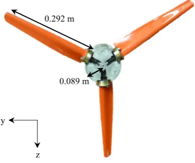
5 Figure 1. Turbine rotor with the nose cone removed.

Table 1 outlines the rotor geometry, and Table 2 presents the geometry of the tested blades (blade twist and chord as functions of radial location). The angle between the rotor plane and the blade at any radial position was defined by adding the values of twist to the root pitch angle given in Table 1.

Table 1 - General dimensions and uncertainties of the rotor ROTOR RADIUS BLADE LENGTH ROOT PITCH SETTING 0.381 ± 0.0005 m 0 .292 ± 0.0005 m 28 ° ± 0.875°

`

Table 2. Geometry of NREL S814 blades

RADIUS (m) TWIST (DEGREES) CHORD (m)

0.089 0 0.0643

0.114 -4.38 0.0629

0.149 -10.74 0.0598

0.183 -14.80 0.0560

0.216 -17.33 0.0516

0.251 -18.91 0.0473

0.286 -19.75 0.0426

0.321 -20.39 0.0381

0.355 -20.87 0.0337

0.381 -21.11 0.0249

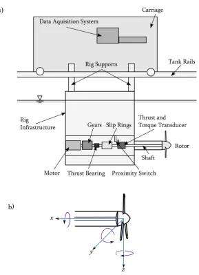
Figure 2 shows the experimental configuration tested in the 76 m by 4.6 m by 2.5 m tow tank at the University of Strathclyde.

0.292 m

y

0.089 m

6 Figure 2. (a) Tow tank carriage and turbine test setup (b) coordinate system.

A motor was used to drive the rotor at a constant rotational speed while the torque was measured with the thrust and torque transducer. A 10:1 gear box was used to step down the rotational speed of the motor to give that of the rotor. A Futek FSH00747 torque and thrust biaxial sensor was used to measure the thrust and the torque on the rotor system. An IS 1163 SW 110/20 CAT slip ring was used to feed the electrical signal from the rotating dynamometer and strain gauges to the data acquisition (DAQ) system.

A proximity sensor was used as a pulse counter to count the number of shaft revolutions in a given time period. Data was logged using a Cambridge Electronic Design Power 1401 DAQ and the DAQ program, Spike, and exported as text files for post processing in MATLAB®. The motor, slip ring, and thrust and torque sensors were enclosed in a submerged container,

a)

7 which was rigidly mounted to the carriage and located approximately 2 diameters downstream of the rotor.

Strain gauges attached to the blade root were used to measure the axial (blade 1 and 2) and radial (blade 3) blade root bending moments. The strain gauges were positioned on cylindrical steel transducers which were isolated from the water with waterproofing material, as shown in Figure 3. The upper section of each steel transducer was bolted firmly to a brass flange and pin designed to enable an accurate pitch setting.

Figure 3. Photograph of hub, bending moment transducer and blade, viewed in axial plane (along the x-axis).

To firmly connect the blade and hub in all degrees of freedom, bolts were secured through the flanges and the pin was slotted into a hole drilled on the bottom-side of the blades at a point on the chord line. The position of this pin hole on the chord line of the blade coincided with the midpoint of the hub depth.

Considerable effort was given to ensuring each blade was set at the same root pitch setting, and that the value and uncertainty of the root pitch were quantified. To achieve this, a depth gauge, fixed in the horizontal plane, was used to measure the distance between the edge of the rotor hub and the trailing edge of the blade at the root. The blades were rotated about the pins until this distancewas the same for each blade. These dimensions were input to the original CAD model of the rotor and used to determine the angle between the blade chord-line and the rotor plane. In the CAD, as in the physical turbine, the blades were constrained to have one degree of freedom in rotation about the pin position on the hub. The resulting angle was

Upper section of steel transducer Waterproofing

material

Brass pitch setting

8 obtained from the CAD program. A machining tolerance of 0.0005 m existed for each dimension of the blades. The original machining process and the subsequent drilling of the pin hole resulted in uncertainty between the CAD model and the physical turbine. When this was taken into consideration, the uncertainty in the pitch setting at the root of the blade was ±

0.875°. The quantification of this uncertainty allows accurate turbine modelling in the numerical performance prediction tools, and informs the upper and lower limits of a sensitivity analysis.

2.2.Theory

To facilitate direct comparison of different turbine systems, regardless of size or design, it is recommended by EquiMar [13] that non-dimensionalized turbine performance characteristics should be used. The relevant performance characteristics for the tests presented here are:

 The coefficient of power, CP, which describes the efficiency of a rotor in capturing the

available energy in a stream tube of the same diameter. CP is defined as

P 3 1 2 Q C Au     (1)

 The coefficient of thrust, CT, which describes the axial thrust experienced by the rotor,

caused by the change in fluid pressure. CT is defined as

T T 2 1 2 F C Au    (2)  The coefficient of blade root bending moment in both the axial and radial directions,

CMy and CMx respectively, which are defined as

y My 2 1 2 M C ARu    (3) x Mx 2 1 2 M C ARu    (4)  The tip speed ratio, λ, which is the ratio between the tangential velocity of the blade

9

R u

 

 

(5) Where is the tow tank carriage speed, Ω is the rotational velocity of the rotor, Q is the rotor torque, FT is the rotor thrust, and Mx/My are the blade root bending moments. The

relationship between CP or CT and λ shows the turbine performance over the range of flow

conditions, and is the most common way of presenting the power-capture capabilities and structural loads expected for a turbine rotor.

2.3.Design of Experiment

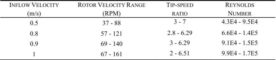
The desired output of this test program was a set of fully-characterized performance curves for the rotor. Four rotor inflow speeds (i.e. carriage tow velocities) were used: 0.5 m/s, 0.8 m/s, 0.9 m/s and 1 m/s. For each inflow speed, a range of rotational velocities, shown in Table 3, were utilized to sufficiently populate the rotor performance curves and clearly characterize the performance and load trends of the turbine. Chord-Reynolds numbers are given in Table 3 and show the range of Reynolds numbers at 75% radius, where the chord length is 0.0421 m.

Table 3. Fluid and rotational velocities used in testing program. INFLOW VELOCITY

(m/s)

ROTOR VELOCITY RANGE

(RPM)

TIP-SPEED RATIO

REYNOLDS

NUMBER

0.5 37 - 88 3 - 7 4.3E4 - 9.5E4

0.8 57 - 121 2.8 - 6.29 6.6E4 - 1.4E5

0.9 69 - 140 3 - 6.29 9.1E4 - 1.5E5

1 67 - 161 2 - 6.51 9.9E4 - 1.7E5

This test program was designed observing the requirements outlined in EquiMar Deliverable D3.4, "Best practice for tank testing of small marine energy devices" [14]. Tests were run in a non-sequential order, and were scheduled (blocked) to avoid random errors such as time of day (affecting steadiness of tank), carriage operators (affecting data collection) and tank temperature (varying over the day). By choosing the tow and rotor velocities of the tests at random, it was also ensured that any sources of uncertainty described as “nuisance factors” in the EquiMar Best Practices document [14] could be eliminated.

To ascertain the repeatability of the tests, a number of repeat runs were performed. In particular one set of conditions, with an inflow velocity of 1 m/s and rotor velocity of 110.7 RPM, was repeated 5 times.

10 Several test sets were run in which the inflow speed was fixed and the rotor velocity varied, producing a fully defined performance curve for the turbine at each inflow speed. Data collection was started in the DAQ programme, Spike, before the carriage was accelerated to test velocity to obtain a steady zero reading for all sensors. During this period, the rotor was spun by the motor at 3 RPM. Collection of offset zero values for the measurement equipment were obtained while the rotor was spinning slowly to allow any rotor misalignments or buoyancy forces to be recorded and their effects considered. With the exception of the rotor velocity, it was assumed that the mean values of the recorded data were zero at this very low rotational speed and that, due to the care taken to ensure appropriate calibration and amplification factors, all noise in the data was Gaussian and could therefore be assumed to be zero over the mean. A motor control curve (voltage waveform text file) was input to Spike to ramp up the rotor rotational speed gradually and keep it constant over the test run. As shown in Figure 4, the carriage was ramped up to the desired inflow speed once the rotor rotational speed was steady. Figure 4 shows the carriage and rotational velocity output data from one of the 0.9 m/s tests.

Figure 4. Carriage velocity and rotor rotational velocity, live data output from test. The carriage was towed down the length of the tank, and gradually slowed near the end. The rotor was ramped down once the carriage stopped, and the tank water was allowed to settle before the next test was run. In the test run illustrated in Figure 4, the zero region occurred between time t=0 s and t=20 s, and the steady region was taken between t=55 s and t=85 s,

0 20 40 60 80 100 120 140 160

-0.2 0 0.2 0.4 0.6 0.8 1 1.2

0 25 50 75 100 125

Rotor

con

trol

cu

rve

(RPM)

Inflow

v

elocity

(ms -1)

Time (s)

11 giving a total time of 30 s at steady carriage (inflow) and rotational velocities. The small drops in the rotor velocity over the course of the test were from electrical noise, and did not influence the actual rotor velocity.

2.5.Post-processing

Measurements from the thrust and torque sensors, bending moment gauges, proximity switch (at a rate of 1 pulse-per-revolution), and motor encoder (at a rate of 10 pulses-per-revolution) were output, along with a timestamp, to a text file during testing. The binary pulse voltage signal from the proximity switch was used to define the start of each rotor revolution such that data could be averaged over full revolutions. The carriage velocity, rotor torque, thrust, and blade root bending moment outputs were averaged over an integer number of rotor revolutions in the steady section of each test (once both the rotor and carriage were operating at steady velocities). The mean zero values for each measurement were subtracted from these average values to correct for measurement offsets.

The binary pulse signals from the proximity switch and motor encoder, along with the time stamp, were used to calculate a moving average of the rotor rotational velocity during the steady section of each test, giving a visual check on the steadiness of the rotor velocity. The mean rotor velocity was calculated from this moving average rotor velocity, and λ was calculated according to Eq. (5). The standard deviation of this moving average rotor velocity was calculated and used to express the uncertainty in the measurement of rotor velocity,

 

std

   .

3. Uncertainty analysis

For each test run, the uncertainty associated with the calculated parameters caused by the bias and precision uncertainties in the instruments, was calculated. This section describes the how these uncertainty estimates were made.

3.1.Uncertainty in calibration

12 the test runs; a reading for thrust force in Newtons is easier to check for accuracy than a reading in volts.

The calibration of torque is used as an example for the uncertainty analyses method employed. To calibrate the torque sensor, known torque loads, Q_applied, were applied to the stationary rotor and the output voltage, V_measured, was recorded. A linear regression analysis of the various applied torques and resulting voltages showed a highly linear calibration curve, well-fitted to the data (with coefficients of determination, R2, above 0.99). During testing, the voltage readings were converted to torque measurements by applying a linear calibration equation of the form V_measured bQ_applieda, where b was the slope and a theoffset constant. The uncertainty associated with this calibration curve was found based on the standard error of estimate, as outlined in the ITTC’s document "Uncertainty Analysis Instrument Calibration" [15]. The summed square of residuals (SSR) is defined as:





R

2

SS ₁

n

i i

i

x





y a bx

 

where x is the known value, y is the measured value, there are n sample points (where i is the sample number), and a and b are from the linear calibration equation. The document [15] states that the standard error of estimate (SEE) is "a measure of the standard deviation for the linear regression analysis", and is defined as:

R

SS SEE

2

x x

n



 (7)

The precision uncertainty,_{P,calibration, Q}, associated with the linear regression method of calibration of torque was determined from:

P,calibration, Q xSEE

  (8)

The total bias uncertainty in the torque measurement (for example from the uncertainty in the mass of the calibration weights used), was calculated by the law of propagation of uncertainty, as detailed in [16], and outlined in EquiMar Deliverable D 3.4 [14]. During calibration, the torque, Q_applied, was calculated from:

applied

13 Where m was the mass of the weight applied during calibration with a bias uncertainty of

Bm

 =0.015 kg, g was the gravitational constant with a bias uncertainty of _Bg=0.001 m/s2, and l was the moment arm with a bias uncertainty of _Bl=0.0005 m. The calculation of the total bias uncertainty in the torque measurement,_{B,calibration, Q}, in Nm, was based on the bias uncertainty for each of these variables, and is expressed as:

2

2 2

Bg

Bm Bl

B,calibration, Q Qapplied _m2 _g2 _l2 

 

    (10)

Combining the precision and bias uncertainties according to the method outlined in [14], the total uncertainty, in Nm, associated with the calibration of torque was calculated by:

2 2

Q,calibration P,calibration,Q B,calibration,Q







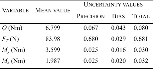
The uncertainty in each of the calibrated instruments was found in this manner, and the uncertainty values for each measured variable are given in Table 4.

Table 4. Uncertainty values from calibration

VARIABLE MEAN VALUE UNCERTAINTY VALUES

PRECISION BIAS TOTAL

Q (Nm) 6.799 0.067 0.043 0.080 FT (N) 83.98 0.680 0.029 0.681

My (Nm) 3.599 0.025 0.016 0.030 Mx (Nm) 1.987 0.025 0.020 0.032

The data in Table 4 showed that the total (combined bias and precision) uncertainty in the calibration of each instrument was two orders of magnitude smaller than the associated mean value of that measurement, providing confidence in the calibration process.

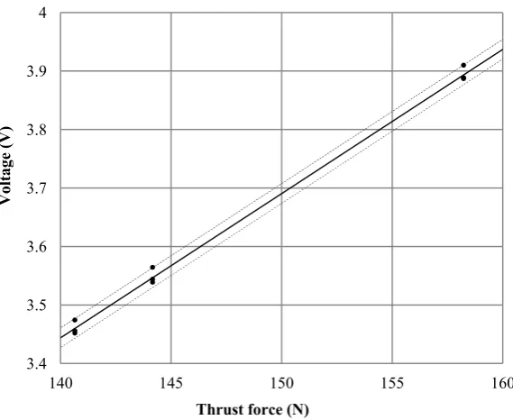
14 Figure 5. Thrust calibration curve with bounding uncertainty lines.

Figure 5 illustrates that all data points fall within the uncertainty bounds, highlighting the low level of scatter in the calibration test data.

3.2.Uncertainty in calculated parameters

For each test the uncertainty in the final calculated results, from the bias and precision uncertainties in the instruments, was calculated using the method of propagation of uncertainty, as previously described. For example, the uncertainty of CP,C_P, was a function

of the uncertainty in each of the parameters used to calculate CP from Eq. (1), and is given by:

B B

P

2 2

2 2 ₂

ρ Q,calibration

2 A 2

C P

mean mean ,mean

3 _U

C

Q A U

 

  



 





 

 

    _{ }

   _    _ _  _ _

        (12)

Values with the subscript “mean” were the average value of each measurement, taken when the carriage and rotor velocities were steady during each test run. This gave the uncertainty in the calculated value for CP.

The same process was undertaken for each of the required experimental outputs.

4. Results

Figure 6 and Figure 7 show CP and CT as a function of λ. 3.4

3.5 3.6 3.7 3.8 3.9 4

140 145 150 155 160

Voltage

(V)

15 Figure 6. CP – λ curve for varying inflow speeds.

Figure 6 shows that a general trend for each of the four tow velocities presented, with some mild scatter in the data. The efficiency of the rotor increased with increasing λ, peaked and then began decreasing. The peak efficiency occurred at a λ of 4.08 for the 0.8 m/s tests, with a

CP of 0.263; at a λ of 3.90 for the 0.9 m/s tests, with a CP of 0.274; and at a λ of 3.53 for the 1

m/s tests, with a CP of 0.285.

Figure 7. CT – λ curve for varying inflow speeds.

From Figure 7, CT for the rotor increased steeply before leveling off and peaking at a λ of

approximately 4.5. After which CT decreased to about 0.40. Comparison between the plots of 0

0.05 0.1 0.15 0.2 0.25 0.3 0.35 0.4

2 3 4 5 6 7

Cp

λ

0.5m/s 0.8m/s

0.9m/s 1 m/s

0.2 0.25 0.3 0.35 0.4 0.45 0.5

2 3 4 5 6 7

CT

λ

0.5m/s 0.8m/s

16

CP and CT showed that, for each flow speed, the peak power capture efficiency of the rotor

roughly coincided with the transition from steep to more shallow increase in CT.

Figure 8 and Figure 9 show the axial and radial root bending moment coefficients.

Figure 8. CMy – λ curve for varying inflow speeds.

Figure 9. CMx – λ curve for varying inflow speeds.

From Figure 8, the coefficient of axial bending moment increased steeply from 0.042 at the lowest λ, to 0.081 at a λ of 3.5, a 93% increase. For λ between 3.5 and 6.4, there was a relatively small increase in bending moment coefficient (1.34 % increase). From Figure 9, the coefficient of bending moment decreased initially until λ of about 3.5, then increased

0 0.02 0.04 0.06 0.08 0.1 0.12

2 3 4 5 6 7

CMy

λ

0.5m/s 0.8m/s 0.9m/s 1 m/s

-0.06 -0.04 -0.02 0 0.02 0.04 0.06

2 3 4 5 6 7

CMx

λ

17 continuously, reaching a maximum of 0.014 at a λ of 6.5. The difference between the 0.5 m/s tests and the higher inflow speed tests is thought to be due to Reynolds number effects, which are discussed in Section 5

4.1.Uncertainty analysis results

Figure 10 shows the percentage uncertainty in CP, CT and λ as a function of tip speed ratio.

Figure 10. Percentage uncertainty for calculated parameters.

The uncertainty in CT and λ was consistently under 1.7%. As shown in Figure 10, there was a

greater percentage uncertainty in CP at very low and very high λ, where the values of CP were

small. The uncertainty in CP was less than 5% for tests below λ of 5.3, with a maximum

uncertainty in CP of 6.8% at the maximum λ. This gave an overall uncertainty in the CP values

of less than 5% for 87% of the tests.

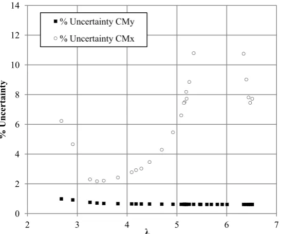
Figure 11 shows the percentage uncertainty in CMy and CMx as a function of λ. 0

2 4 6 8 10 12 14

2 3 4 5 6 7

%

Un

certain

ty

λ

18 Figure 11. Percentage uncertainty for calculated parameters.

The uncertainty in CMy was consistently less than 1.4% for over 93% of the tests done. From

Figure 11, CMx had the largest percent uncertainty; over 15% for 37% of the tests. As Table 4

shows, the combined uncertainty in the calibration of the radial blade root bending moment, CMx, was of the same order of magnitude as that of the axial blade root bending moment, CMy;

however, the measured radial bending moments were small, making the percentage uncertainty much higher than for the other measurements.

The standard deviations of the CP, CT, CMx, CMy and λ for the 5 repeated tests were compared

with the set’s minimum uncertainty for each variable. Comparing the standard deviation to the minimum uncertainty indicated if the experimental scatter was within the calibration-based uncertainty bounds, giving a conservative analysis of the repeatability of the tests. Table 5 shows the standard deviation and the minimum uncertainty for each parameter over the 5 tests.

Table 5 - Results of the repeatability analysis.

PERFORMANCE CHARACTERISTIC STANDARD DEVIATION MINIMUM UNCERTAINTY

CP 0.0013 0.0044

CT 0.0017 0.0039

λ 0.0014 0.0077

CMx 7.5e-5 0.00038

CMy 1.7e-4 0.00063

0 2 4 6 8 10 12 14

2 3 4 5 6 7

%

Un

certain

ty

λ

% Uncertainty CMy

19 The repeatability analysis showed that, for each of the performance characteristics, the standard deviation of the values in the set of repeated tests fell within the bounds of the known uncertainty associated with that value, illustrating the high repeatability of the results.

5. Discussion

The aim of this test program was to obtain high quality data to use for verification and calibration of performance models. The optimum root pitch angle was not pre-determined. This reduced the maximum CP and CT to values below the theoretical maximum for these

blades. This test data is therefore not presented to showcase the optimum performance of NREL S814 blades, but rather to empirically quantify their performance.

For this system, the rotor-tank blockage ratio was 4.47%; evidence from the literature suggested that it was not necessary to apply any correction.

A small amount of noise was captured in the data, however, this noise was of equal amplitude above and below the data mean, and the processing method ensured data was averaged over a full rotation of the rotor. Therefore, it was deemed acceptable to take the mean values of the data captured without applying a filter.

The efficieny of the rotor presented was well below Betz limit of 0.59 [17]. This is thought to be due to high frictional losses in the system, a non-optimum root pitch setting, and low Reynolds number operational effects. Losses in a scale model test have a higher impact on test results than in larger systems due to a higher ratio between frictional losses and the captured power. The performance of the blade airfol shape, which is dependant on the chord Reynolds number, also influenced power capture. Reynolds number matching for small scale tidal turbines is limited at most test facilities due to carriage and rotational velocity constraints. For this work, due to the small scale of the turbines being tested, the operational range of Reynolds numbers was low. In the lower Reynolds-number ranges, airfoil performance is degraded and unusual performance characteristics can develop, caused by different effects of transition, laminar separation, and laminar bubble behavior [18]. The differences between the performance curves obtained at different carriage speeds –particularly between the 0.5 m/sCP-λ curve and those of the higher inflow speed tests - highlight the

Reynolds number sensitivities. As the inflow speed and Reynolds number increased, the turbine became more efficient and the optimum λ decreased. At higher inflow speeds, the

CP-λ curves began to converge, as seen in Figure 6. According to experimental research

20 occured on the upper and lower airfoil surface due to the thickness of the airfoil, which is thought to have influenced the performance of the NREL S814 airfoil. These effects may have also varied with Reynolds number, however, this was not investigated at this time.

Carriage vibrations, speed tolerances, and uniformity can affect the accuracy of speed control and the length of time for data collection at a constant speed. However, in this test setup, the uncertainty in λ was shown to be consistently below 1.7%. This low uncertainty, due to the high precision in the carriage speed, confirms that the quality of the inflow velocity and rotor speed did not negatively influence the test results. Due to the high frequency of data capture, and the length of time at steady state in the tow tank facility, it was possible to obtain large sample numbers. This ensured that the effect of any fluctuations would be negated over the test period. As Figure 4 shows, both the carriage speed and the motor rotational speed input were maintained at steady values over the steady region.

6. Conclusions

An experimental dataset for a small scale tidal turbine with quantified uncertainty was produced in the tow tank at Strathclyde University. This data will be used for verification of a BEMT-based performance tool and will form a base-case for the development of new blade design methodologies. The rotor performance has been characterized over a full range of operational tip speed ratios for carriage speeds of 0.5, 0.8, 0.9 and 1 m/s. A maximum CP of

0.285 and a maximum CT of 0.452 were recorded at λ of 3.53 and 4.45 for the 1 m/s carriage

speed.

Uncertainty analyses were undertaken to give confidence in the methods and data produced. The uncertainty in the measurements were found to be less than 5% for over 87% of the tests, with the higher uncertainty coming from tests with very small measured values, such as Cp

21

Acknowledgments

The authors would like to acknowledge the involvement and support of the staff at Strathclyde University; Sandy Day, Charles Kay, Ed Nixon Grant Dunning and the rest of the team at Achre Road. Our thanks also go to Steve Martin for his contributions in this test series. Finally, we gratefully thank OREA, the United Kingdom Science and Innovation Network, Scottish Development International, NSERC and RCUK SuperGen for their support.

References

1. The European Marine Energy Centre (EMEC), Guidelines for Reliability, Maintainability and

Survivability of Marine Energy Conversion Systems, 2009.

2. I. A. Milne, A. H. Day, R. N. Sharma, and R. G. J. Flay, Blade loads on tidal turbines in planar oscillatory flow. Ocean Engineering, 2013. 60: p. 163-174.

3. W. M. J. Batten, A. S. Bahaj, A. F. Molland, and J. R. Chaplin, The prediction of the hydrodynamic performance of marine current turbines. Renewable Energy, 2008. 33(5): p. 1085-1096.

4. Chul Hee Jo, Jin Young Yim, Kang Hee Lee, and Yu Ho Rho, Performance of horizontal axis tidal current turbine by blade configuration. Renewable Energy, 2012. 42: p. 195-206.

5. J.A. Clarke, G. Connor, A.D. Grant, C. Johnstone, and D. Mackenzie, Development of a contra-rotating tidal current turbine and analysis of performance, in EWTEC, 2007: Southampton , UK.

6. Luke E. Myers Pascal W. Galloway, Abubakr S. Bahaj. Experimental and numerical results of rotor power and thrust of a tidal turbine operating at yaw and in waves, in WREC, 2011. Sweden

7. F. Maganga, G. Germain, J. King, G. Pinon, and E. Rivoalen, Experimental characterisation of flow effects on marine current turbine behaviour and on its wake properties. IET Renewable Power Generation, 2010. 4(6): p. 498.

8. T. Mccombes, et al., EquiMar Deliverable 3.3 Assessment of current practice for tank testing of small marine energy devices, in Equitable Testing and Evaluation of Marine Energy Extraction Devices in terms of Performance, Cost and Environmental Impact, 2010.

9. MARINET - Marine Renewables Infrastructure Network for Emerging Energy Technologies 2015; Available from: http://www.fp7-marinet.eu/standardisation&bestpractice_tidal_energy.html.

10. Pascal Galloway, Luke Myers, and Abubakr Bahaj, Operational issues surrounding the use of towing tanks for performance quantification of marine current energy converters, in EWTEC, 2011: Southhampton, U.K. .

11. R. J. Poole and I. Owen S. C. Tedds. Wake characteristics of Horizontal Axis Tidal Stream Turbines in uniform and non-uniform steady flows, in 4th International Conference on Ocean Energy, 2012,Dublin, Ireland.

12. A. S. Bahaj, W. M. J. Batten, and G. Mccann, Experimental verifications of numerical predictions for the hydrodynamic performance of horizontal axis marine current turbines. Renewable Energy, 2007.

32(15): p. 2479-2490.

13. J.A. Clarke, et al., EquiMar Deliverable 3.2 Concept Appraisal and Tank Testing Practices for 1st Stage Prototype Devices, in Equitable Testing and Evaluation of Marine Energy Extraction Devices in terms of Performance, Cost and Environmental Impact, 2009.

14. T. Mccombes, et al., EquiMar Deliverable 3.4 Best practice for tank testing of small marine energy devices, in Equitable Testing and Evaluation of Marine Energy Extraction Devices in terms of Performance, Cost and Environmental Impact, 2010.

15. International Towing Tank Conference "Specialist Committee on Uncertainty Analysis", Recommended Procedures and Guidelines Uncertainty Analysis and Instrument Calibration, 2008.

16. National Institute of Standards And Technology, Engineering Statistics Handbook- Propagation of error for many variables, 2014.

22

Atrium, Southern Gate, Chichester, West Sussex PO 19 8SQ, England: John Wiley & Sons, Ltd.

18. Ian Angus Milne, An Experimental Investigation of Turbulence and Unsteady Loading on Tidal