A Stochastic Differential Equation SIS
Epidemic Model
A. Gray
1, D. Greenhalgh
1, L. Hu
2, X. Mao
1,∗, J. Pan
11
Department of Mathematics and Statistics,
University of Strathclyde, Glasgow G1 1XH, U.K.
2Department of Applied Mathematics,
Donghua University, Shanghai 201620, China.
Abstract
In this paper we extend the classical SIS epidemic model from a deterministic framework to a stochastic one, and formulate it as a stochastic differential equation
(SDE) for the number of infectious individuals I(t). We then prove that this SDE
has a unique global positive solution I(t) and establish conditions for extinction
and persistence ofI(t). We discuss perturbation by stochastic noise. In the case of
persistence we show the existence of a stationary distribution and derive expressions for its mean and variance. The results are illustrated by computer simulations, including two examples based on real life diseases.
Key words: SIS model, Brownian motion, stochastic differential equations, ex-tinction, persistence, basic reproduction number, stationary distribution, gonorrhea, pneumococcus.
1
Introduction
Epidemics are commonly modelled by using deterministic compartmental models where the population amongst whom the disease is spreading is divided into several classes, such as susceptible, infected and removed individuals. The classical Kermack-McKendrick model [15] is sometimes used for modelling common childhood diseases where a typical individual starts off susceptible, at some stage catches the disease and after a short infec-tious period becomes permanently immune. This is sometimes called the SIR (susceptible-infected-removed) model.
However some diseases, in particular some sexually transmitted and bacterial diseases, do not have permanent immunity. For these diseases individuals start off susceptible, at some stage catch the disease and after a short infectious period become susceptible again. There is no protective immunity. For these diseases SIS (susceptible-infected-susceptible)
models are appropriate [14]. If S(t) denotes the number of susceptibles and I(t) the
number of infecteds at time t, then the differential equations which describe the spread of the disease are:
( dS(t)
dt =µN−βS(t)I(t) +γI(t)−µS(t), dI(t)
dt =βS(t)I(t)−(µ+γ)I(t),
(1.1)
with initial values S0 +I0 = N. N is the total size of the population amongst whom
the disease is spreading. Here µ is the per capita death rate, and γ is the rate at which
infected individuals become cured, so 1/γ is the average infectious period. β is the disease
transmission coefficient, so thatβ =λ/N whereλis the per capita disease contact rate. λ
is the average number of adequate contacts of an infective per day. An adequate contact is one which is sufficient for the transmission of an infection if it is between a susceptible and an infected individual. This is one of the simplest possible epidemic models and because it is so simple it and its variants are commonly studied. For example, SIS models are discussed by Brauer et al. [2]. There are many other examples of SIS epidemic models in the literature.
In their excellent monograph Hethcote and Yorke [14] outline several mathematical models for gonorrhea with increasing levels of complexity. The simplest of these is the
above model (1.1) with µ set to zero (i.e. no demography). As S +I = N, the total
population is constant, the two models with and without demographics are equivalent; just
replaceγ in the model with no demography byµ+γ to get the model with demography.
This is a very simple model for gonorrhea. It assumes that the population is homoge-neous (so is more suitable for a homosexual than a heterosexual population) and mixing is homogeneous, whereas in practice sexual mixing is extremely heterogeneous. It also ignores the small but non-zero disease incubation period and assumes that contact rates remain constant and do not vary seasonally. Lajmanovich and Yorke [17] and Nold [28] discuss heterogeneously mixing SIS epidemic models for the spread of gonorrhea. The model (1.1) also ignores screening. Hethcote and Yorke define the contact number to be
σ =λ/γ, so in our model σ=βN/(µ+γ).
If ˜I =I/N is the fraction of the population infected at timet then they show that in
our notation the solution is
I(t) =
h
β
βN−µ−γ(1−e
−(βN−µ−γ)t) + 1
I0e
−(βN−µ−γ)ti−1, if βN µ+γ 6= 1,
h
βt+ 1
I0
i−1
, if µβN+γ = 1.
(1.2)
It is straightforward to show that σ has the usual interpretation as the basic
repro-duction numberR0. This is the expected number of secondary cases produced by a single
newly infected individual entering a disease-free population at equilibrium. In such a
situation each newly infected individual remains infectious for time 1/(µ+γ) and during
this period infects βN of the N susceptibles present. Hence
R0 =σ=
βN
µ+γ. (1.3)
From now on we denote this R0 by RD0 to emphasise that it is R0 for the deterministic
• IfRD
0 ≤1, limt→∞I(t) = 0.
• IfRD
0 >1, limt→∞I(t) =N
1− 1
RD
0
.
Another disease for which it is possible to use an SIS model is pneumococcal carriage.
Streptococcus pneumoniae (S.pneumoniae) is a bacterium commonly found in the throat
of young children. When an individual carries pneumococcus the infectious carriage nor-mally lasts around 7 weeks [30] and at the end of this carriage period the individual is
susceptible again. R0 for pneumococcal carriage and transmission is 1.8-2.2 [32]. Lipsitch
[20] discusses mathematical models for the transmission of S.pneumoniae with multiple
serotypes and vaccination. Lamb, Greenhalgh and Robertson [18] discuss a mathematical
model for the transmission of a single serotype of S.pneumoniae with vaccination. If
we have only a single serotype and no vaccination then the disease can be modelled by equations (1.1). Other bacterial diseases, for example tuberculosis, can be modelled by SIS models [9].
Allen [1] discusses a stochastic model of the above SIS epidemic model. However this is done by constructing a stochastic differential equation (SDE) approximation to the continuous time Markov Chain model. The latter is obtained by assuming that events oc-curring at a constant rate in the deterministic model occur according to a Poisson process with the same rate. McCormack and Allen [27] construct a similar SDE approximation to an SIS multihost epidemic model and explore the stochastic and deterministic models numerically. However this is not the only way to introduce stochasticity into the model, and in this paper we explore an alternative, namely parameter perturbation.
We have previously used the technique of parameter perturbation to examine the effect of environmental stochasticity in a model of AIDS and condom use [5]. We found that the introduction of stochastic noise changes the basic reproduction number of the disease and can stabilise an otherwise unstable system. Ding, Xu and Hu [6] apply a similar technique to a simpler model of HIV/AIDS transmission. Other previous work on parameter perturbation in epidemic models seems to have concentrated on the SIR model. Tornatore, Buccellato and Vetro [29] discuss an SDE SIR system with and without delay with a similar parameter perturbation as we shall discuss here. The system for the SDE SIR model with no delay is
dS˜(t) = [µ−β˜S˜(t) ˜I(t)−µS˜(t)]dt−σ˜S˜(t) ˜I(t)dB(t),
dI˜(t) = [ ˜βS˜(t) ˜I(t)−(µ+γ) ˜I(t)]dt+ ˜σS˜(t) ˜I(t)dB(t),
dR˜(t) =γI˜(t)−µR˜(t),
(1.4)
where B(t) is a Brownian motion. Here ˜S,I˜and ˜R denote respectively the susceptible,
infected and removed fractions of the population, rather than absolute numbers, so that ˜
β in this model corresponds to βN in (1.1). They study the stability of the disease-free
equilibrium (DFE). They find that
0<β <˜ min
γ+µ− σ˜
2
2 ,2µ
introduction of noise into the system raises the threshold toµ+γ+ (˜σ2/2), so if
min
µ+γ− σ˜
2
2 ,2µ
<β < γ˜ +µ+ σ˜
2
2
then the DFE E0 = (S(0), I(0), R(0)) = (1,0,0) is stable and the disease does not occur,
whereas if ˜β > γ+µ+ (˜σ2/2) then the DFE is unstable. These results are similar to those
of [5]. Chen and Li [4] study an SDE version of the SIR model both with and without delay, but introduce stochastic noise in a different way than we and Tornatore, Buccellato and Vetro [29] do. Lu [22] studies an SIRS (susceptible-infected-removed-susceptible) model which generalises the model of [29] by allowing removed individuals to become susceptible again. He extends their results by including the possibility that immunity is only temporary and improving the analytical bound on the sufficient condition for the
stability of the DFE to β < µ+γ −(˜σ2/2).
In summary the deterministic SIS epidemic model is one of the simplest possible epi-demic models, which has applications to transmission of real-life diseases, such as pneu-mococcus, gonorrhea and tuberculosis. It is important to include the effect of uncertainty in estimation of parameters such as the disease transmission coefficient. Whilst several papers study the effect of stochastic parameter perturbation on SIR and SIRS epidemic models, we are not aware of any literature addressing this issue in SIS epidemic models. This paper is an attempt to fill this gap.
2
Stochastic Differential Equation SIS Model
Throughout this paper, we let (Ω,F,{Ft}t≥0,P) be a complete probability space with a
filtration {Ft}t≥0 satisfying the usual conditions (i.e. it is increasing and right continuous
whileF0 contains allP-null sets) and we letB(t) be a scalar Brownian motion defined on
the probability space. We use a∨b to denote max(a, b), a∧b to denote min(a, b), and
a.s. to mean almost surely. We will denote the indicator function of a set G byIG.
Let us now consider the second equation of (1.1). To establish the stochastic dif-ferential equation (SDE) model, we naturally re-write this equation in the difdif-ferential form
dI(t) = [βS(t)I(t)−(µ+γ)I(t)]dt. (2.1)
Here [t, t+dt) is a small time interval and we use the notationd·for the small change
in any quantity over this time interval when we intend to consider it as an infinitesimal
change, for example dI(t) = I(t+dt)−I(t) and the change dI(t) is described by (2.1).
Consider the disease transmission coefficient β in the deterministic model. This can be
thought of as the rate at which each infectious individual makes potentially infectious contacts with each other individual, where a potentially infectious contact will transmit the disease if the contact is made by an infectious individual with a susceptible individual.
Thus the total number of new infections in the small time interval [t, t+dt) is
βS(t)I(t)dt
βdt
potentially infectious contacts with each other individual in the small time interval [t, t+
dt).
Now suppose that some stochastic environmental factor acts simultaneously on each
individual in the population. In this case β changes to a random variable ˜β. More
precisely each infected individual makes
˜
βdt =βdt+σdB(t)
potentially infectious contacts with each other individual in [t, t+dt). HeredB(t) = B(t+
dt)−B(t) is the increment of a standard Brownian motion. Thus the number of potentially
infectious contacts that a single infected individual makes with another individual in
[t, t+dt) is normally distributed with meanβdt and variance σ2dt. Hence E( ˜βdt) =βdt
and var( ˜βdt) = σ2dt. As var( ˜βdt) →0 as dt→ 0 this is a biologically reasonable model.
Indeed this is a well-established way of introducing stochastic environmental noise into biologically realistic population dynamic models. See [7, 10, 11, 12, 19, 22, 29] and many other references.
To motivate our assumption we argue as follows. Suppose that the number of po-tentially infectious contacts between an infectious individual and another individual in
successive time intervals [t, t+T),[t+T, t+ 2T), . . . ,[t+ (n−1)T, t+nT) are
indepen-dent, identically distributed random variables and n is very large. Then by the Central
Limit Theorem the total number of potentially infectious contacts made in [t, t+nT)
has approximately a normal distribution with mean nµ0 and variancenσ20, where µ0 and
σ2
0 are respectively the mean and variance of the underlying distribution in each of the
separate time intervals of lengthT. Thus it is reasonable to assume that the total number
of potentially infectious contacts has a normal distribution whose mean and variance scale as the total length of the time interval as in our assumptions.
Therefore we replace βdt in equation (2.1) by ˜βdt=βdt+σdB(t) to get
dI(t) =S(t)I(t)(βdt+σdB(t))−(µ+γ)I(t)dt. (2.2)
Note that βdt now denotes the mean of the stochastic number of potentially infectious
contacts that an infected individual makes with another individual in the infinitesimally
small time interval [t, t+dt). Similarly, the first equation of (1.1) becomes another SDE.
That is, the deterministic SIS model (1.1) becomes the Itˆo SDE
dS(t) = [µN−βS(t)I(t) +γI(t)−µS(t)]dt−σS(t)I(t)dB(t),
dI(t) = [βS(t)I(t)−(µ+γ)I(t)]dt+σS(t)I(t)dB(t). (2.3)
This SDE is called an SDE SIS model.
Given that S(t) +I(t) = N, it is sufficient to study the SDE for I(t)
dI(t) =I(t)[βN −µ−γ −βI(t)]dt+σ(N −I(t))dB(t) (2.4)
with initial value I(0) =I0 ∈(0, N). In the following sections we will concentrate on this
3
Existence of Unique Positive Solution
The SDE SIS model (2.4) is a special SDE. In order for the model to make sense, we need to show at least that this SDE SIS model does not only have a unique global solution but
also the solution will remain within (0, N) whenever it starts from there. The existing
general existence-and-uniqueness theorem on SDEs (see e.g. [23, 24, 25]) is not applicable to this special SDE in order to guarantee these properties. It is therefore necessary to establish such a new theory.
Theorem 3.1 For any given initial value I(0) =I0 ∈(0, N), the SDE (2.4) has a unique
global positive solution I(t)∈(0, N) for all t≥0 with probability one, namely
P{I(t)∈(0, N) for all t≥0}= 1.
Proof. Regarding equation (2.4) as an SDE on R, we see that its coefficients are locally Lipschitz continuous. It is known (see e.g. [23, 24, 25]) that for any given initial value
S0 ∈ (0, N) there is a unique maximal local solution I(t) on t ∈ [0, τe), where τe is the
explosion time. Let k0 > 0 be sufficiently large for 1/k0 < I0 < N −(1/k0). For each
integer k ≥k0, define the stopping time
τk = inf{t∈[0, τe) :I(t)6∈(1/k, N −(1/k))},
where throughout this paper we set inf∅ =∞ (as usual, ∅= the empty set). Clearly, τk
is increasing as k → ∞. Set τ∞ = limk→∞τk, whence τ∞ ≤ τe a.s. If we can show that
τ∞ = ∞ a.s., then τe = ∞ a.s. and I(t) ∈ (0, N) a.s. for all t ≥ 0. In other words, to
complete the proof all we need to show is thatτ∞=∞a.s. If this statement is false, then
there is a pair of constants T >0 and ε∈(0,1) such that
P{τ∞ ≤T}> ε.
Hence there is an integer k1 ≥k0 such that
P{τk≤T} ≥ε for all k≥k1. (3.1)
Define a function V : (0, N)→R+ by
V(x) = 1
x +
1
N −x.
By the Itˆo formula (see e.g. [25]), we have, for anyt ∈[0, T] and k ≥k1,
EV(I(t∧τk)) =V(I0) +E
Z t∧τk
0
LV(I(s))ds, (3.2)
where LV : (0, N)→R is defined by
LV(x) = x
− 1
x2 +
1
(N−x)2
[βN −µ−γ−βx]
+ σ2x2(N −x)2
1
x3 +
1
(N −x)3
It is easy to show that
LV(x)≤ µ+γ
x +
βN
N −x +σ
2N2
1
x +
1
N −x
≤CV(x), (3.4)
where C = (µ+γ)∨(βN) +σ2N2. Substituting this into (3.2) we get
EV(I(t∧τk))≤V(I0) +E
Z t∧τk
0
CV(I(s))ds ≤V(I0) +C
Z t
0
EV(I(s∧τk))ds.
The Gronwall inequality yields that
EV(I(T ∧τk))≤V(I0)eCT. (3.5)
Set Ωk = {τk ≤ T} for k ≥ k1 and, by (3.1), P(Ωk) ≥ ε. Note that for every ω ∈ Ωk,
I(τk, ω) equals either 1/k orN −(1/k), and hence
V(I(τk, ω))≥k.
It then follows from (3.5) that
V(I0)eCT ≥E
h
IΩk(ω)V(I(τk, ω)) i
≥kP(Ωk)≥εk.
Letting k→ ∞ leads to the contradiction
∞> V(I0)eCT =∞,
so we must therefore have τ∞=∞ a.s., whence the proof is complete.
4
Extinction
In the study of population systems, extinction and persistence are two of most important issues. We will discuss the extinction of the SDE SIS model (2.4) in this section but leave its persistence to the next section.
Theorem 4.1 If
R0S :=RD0 − σ
2N2
2(µ+γ) =
βN
µ+γ −
σ2N2
2(µ+γ) <1 and σ
2 ≤ β
N, (4.1)
then for any given initial value I(0) =I0 ∈(0, N), the solution of the SDE (2.4) obeys
lim sup
t→∞
1
t log(I(t))≤βN−µ−γ−0.5σ
2
N2 <0 a.s., (4.2)
Proof. By the Itˆo formula, we have
log(I(t)) = log(I0) +
Z t
0
f(I(s))ds+ Z t
0
σ(N −I(s))dB(s), (4.3)
where f :R→R is defined by
f(x) =βN −µ−γ−βx−0.5σ2(N −x)2. (4.4)
However, under condition (4.1), we have
f(I(s)) = βN −µ−γ−0.5σ2N2−(β−σ2N)I(s)−0.5σ2I2(s),
≤ βN −µ−γ−0.5σ2N2,
for I(s)∈(0, N). It then follows from (4.3) that
log(I(t))≤log(I0) + (βN −µ−γ −0.5σ2N2)t+
Z t
0
σ(N −I(s))dB(s). (4.5)
This implies
lim sup
t→∞
1
t log(I(t))≤βN−µ−γ−0.5σ
2N2+ lim sup
t→∞
1 t
Z t
0
σ(N−I(s))dB(s) a.s. (4.6)
But by the large number theorem for martingales (see e.g. [25]), we have
lim sup
t→∞
1 t
Z t
0
σ(N −I(s))dB(s) = 0 a.s.
We therefore obtain the desired assertion (4.2) from (4.6).
It is useful to observe that in the classical deterministic SIS model (1.1), I(t) tends
to 0 if and only if RD0 ≤ 1; while in the SDE SIS model (2.3), I(t) tends to 0 if RS0 =
RD
0 −0.5σ2N2/(µ+γ) < 1 and σ2 ≤ β/N. In other words, the conditions for I(t) to
become extinct in the SDE SIS model are weaker than in the classical deterministic SIS model. The following example illustrates this result more explicitly:
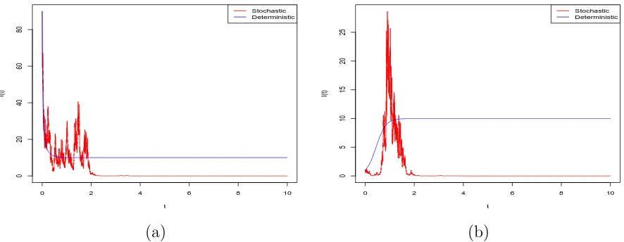
Example 4.2 Throughout the paper we shall assume that the unit of time is one day and the population sizes are measured in units of 1 million, unless otherwise stated. With these units assume that the system parameters are given by
β = 0.5, N = 100, µ= 20, γ = 25, σ = 0.035.
So the SDE SIS model (2.4) becomes
dI(t) = I(t)[5−0.5I(t)]dt+ 0.035(100−I(t))dB(t). (4.7)
Noting that
RS0 = βN
µ+γ −
σ2N2
2(µ+γ) =
50
45 −
12.25
90 = 1.111−0.136 <1,
and σ2 = 0.001225≤ β
we can therefore conclude, by Theorem 4.1, that for any initial valueI(0) =I0 ∈(0,100),
the solution of (4.7) obeys
lim sup
t→∞
1
t log(I(t))≤ −1.125 a.s.
That is,I(t) will tend to zero exponentially with probability one.
On the other hand, the corresponding deterministic SIS model (1.1) becomes
dI(t)
dt =I(t)(5−0.5I(t)). (4.8)
For RD
0 >1, it is known that, for any initial value I(0) = I0 ∈(0,100), this solution has
the property
lim
t→∞I(t) = N
1− 1
RD
0
= 10 (see section 1).
The computer simulations in Figure 4.1, using the Euler Maruyama (EM) method (see e.g. [16, 25, 26]), support these results clearly, illustrating extinction of the disease.
0 2 4 6 8 10
0
20
40
60
80
t
I(t)
Stochastic Deterministic
(a)
0 2 4 6 8 10
0
5
10
15
20
25
t
I(t)
Stochastic Deterministic
[image:9.612.75.518.338.510.2](b)
Figure 4.1: Computer simulation of the pathI(t) for the SDE SIS model (4.7) and its
corresponding deterministic SIS model (4.8), using the EM method with step size ∆ = 0.001,
using initial values (a)I(0) = 90 and (b) I(0) = 1.
In Theorem 4.1 we require the noise intensity σ2 ≤ β/N. The following theorem
covers the case when σ2 > β/N:
Theorem 4.3 If
σ2 > β
N ∨
β2
2(µ+γ), (4.9)
then for any given initial value I(0) = I0 ∈ (0, N), the solution of the SDE SIS model
(2.4) obeys
lim sup
t→∞
1
t log(I(t))≤ −µ−γ+
β2
namely, I(t) tends to zero exponentially almost surely. In other words, the disease dies out with probability one.
Proof. We use the same notation as in the proof of Theorem 4.1. It is easy to see that
the quadratic function f :R→R defined by (4.4) takes its maximum valuef(ˆx) at
x= ˆx:= σ
2N −β
σ2 .
By condition (4.9), it is easy to see that ˆx∈(0, N). Compute
f(ˆx) =βN −µ−γ−0.5σ2N2+(σ
2N −β)2
2σ2 =−µ−γ+
β2
2σ2,
which is negative by condition (4.9). It therefore follows from (4.3) that
log(I(t))≤log(I0) +f(ˆx)t+
Z t
0
σ(N −I(s))dB(s).
This implies, in the same way as in the proof of Theorem 4.1, that
lim sup
t→∞
1
t log(I(t))≤f(ˆx) a.s.,
as required. The proof is hence complete.
Note that condition (4.9) implies that RS
0 ≤1.
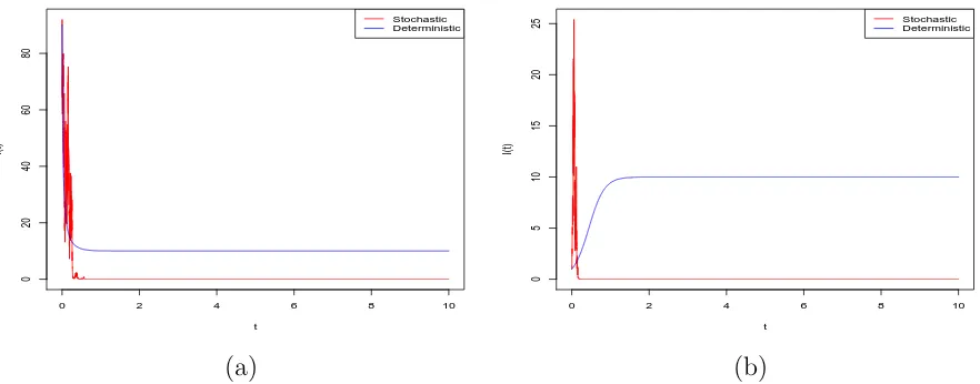
Example 4.4 We keep the system parameters the same as in Example 4.2 but let σ =
0.08, so the SDE SIS model (2.4) becomes
dI(t) =I(t)[5−0.5I(t)]dt+ 0.08(100−I(t))dB(t). (4.11)
It is easy to verify that the system parameters obey condition (4.9). We can therefore
conclude, by Theorem 4.3, that for any initial value I(0) =I0 ∈ (0,100), the solution of
(4.11) obeys
lim sup
t→∞
1
t log(I(t))≤ −45 +
0.52
2×0.082 =−25.4688 a.s.
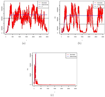
That is, I(t) will tend to zero exponentially with probability one. The computer
simula-tions shown in Figure 4.2 support these results clearly.
5
Persistence
Theorem 5.1 If
RS0 := βN
µ+γ −
σ2N2
0 2 4 6 8 10
0
20
40
60
80
t
I(t)
Stochastic Deterministic
(a)
0 2 4 6 8 10
0
5
10
15
20
25
t
I(t)
Stochastic Deterministic
[image:11.612.77.518.82.255.2](b)
Figure 4.2: Computer simulation of the pathI(t) for the SDE SIS model (4.11) and its
corresponding deterministic SIS model (4.8), using the EM method with step size ∆ = 0.001,
with initial values (a) I(0) = 90 and (b) I(0) = 1.
then for any given initial value I(0) = I0 ∈ (0, N), the solution of the SDE SIS model
(2.4) obeys
lim sup
t→∞
I(t)≥ξ a.s. (5.2)
and
lim inf
t→∞ I(t)≤ξ a.s. (5.3)
where
ξ= 1
σ2
p
β2−2σ2(µ+γ)−(β−σ2N) (5.4)
which is the unique root in (0, N) of
βN−µ−γ−βξ−0.5σ2(N −ξ)2 = 0. (5.5)
That is, I(t) will rise to or above the level ξ infinitely often with probability one.
Proof. Recall the definition (4.4) of functionf :R→R. By condition (5.1), it is easy to
see that equation f(x) = 0 has a positive root and a negative root. The positive one is
1 σ2
p
(β−σ2N)2+ 2σ2(βN −µ−γ −0.5σ2N2)−(β−σ2N)
= 1
σ2
p
β2−2σ2(µ+γ)−(β−σ2N)=ξ.
Noting that
f(0) =βN−µ−γ−0.5σ2N2 >0 and f(N) = −µ−γ <0,
we see that ξ ∈(0, N) and
f(x)>0 is strictly decreasing on x∈(0∨x, ξˆ ), (5.7)
while
f(x)<0 is strictly decreasing on x∈(ξ, N). (5.8)
We now begin to prove assertion (5.2). If it is not true, then there is a sufficiently
small ε∈(0,1) such that
P(Ω1)> ε, (5.9)
where Ω1 ={lim supt→∞I(t)≤ξ−2ε}. Hence, for everyω∈Ω1, there is aT =T(ω)>0
such that
I(t, ω)≤ξ−ε whenever t≥T(ω). (5.10)
Clearly we may chooseεso small (if necessary reduce it) thatf(0)> f(ξ−ε). It therefore
follows from (5.6), (5.7) and (5.10) that
f(I(t, ω))≥f(ξ−ε) whenever t≥T(ω). (5.11)
Moreover, by the large number theorem for martingales, there is a Ω2 ⊂Ω withP(Ω2) = 1
such that for every ω∈Ω2,
lim
t→∞
1 t
Z t
0
σ(N −I(s, ω))dB(s, ω) = 0. (5.12)
Now, fix any ω∈Ω1∩Ω2. It then follows from (4.3) and (5.11) that, fort ≥T(ω),
log(I(t, ω)) ≥ log(I0) +
Z T(ω)
0
f(I(s, ω))ds+f(ξ−ε)(t−T(ω))
+ Z t
0
σ(N −I(s, ω))dB(s, ω). (5.13)
This yields
lim inf
t→∞
1
t log(I(t, ω))≥f(ξ−ε)>0, whence
lim
t→∞I(t, ω) =∞.
But this contradicts (5.10). We therefore must have the desired assertion (5.2).
Let us now prove assertion (5.3). If it were not true, then there is a sufficiently small
δ∈(0,1) such that
P(Ω3)> δ, (5.14)
where Ω3 ={lim inft→∞I(t)≥ξ+ 2δ}. Hence, for every ω ∈Ω3, there is a τ =τ(ω)>0
such that
I(t, ω)≥ξ+δ whenever t≥τ(ω). (5.15)
Now, fix any ω∈Ω3∩Ω2. It then follows from (4.3) and (5.8) that, fort ≥τ(ω),
log(I(t, ω)) ≤ log(I0) +
Z τ(ω)
0
f(I(s, ω))ds+f(ξ+δ)(t−τ(ω))
+ Z t
This, together with (5.12), yields
lim sup
t→∞
1
t log(I(t, ω))≤f(ξ+δ)<0,
whence
lim
t→∞I(t, ω) = 0.
But this contradicts (5.15). We therefore must have the desired assertion (5.3). The proof is therefore complete.
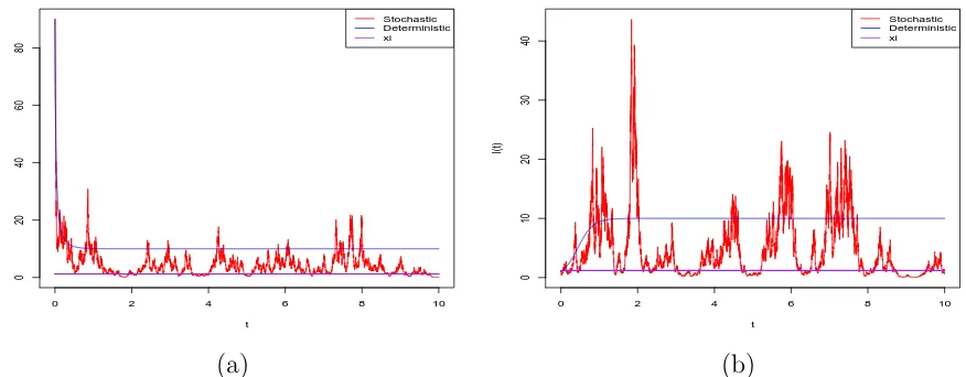
Example 5.2 Assume that the system parameters are given by
β = 0.5, N = 100, µ = 20, γ= 25, σ= 0.03.
That is, we keep all the system parameters the same as in Example 4.2 exceptσ is reduced
to 0.03 from 0.035. So the SDE SIS model (2.4) becomes
dI(t) =I(t)[5−0.5I(t)]dt+ 0.03(100−I(t))dB(t). (5.17)
Noting that
RS0 = βN
µ+γ −
σ2N2
2(µ+γ) =
50
45−0.1>1,
we compute
ξ= 1
σ2
p
β2−2σ2(µ+γ)−(β−σ2N)= 1.2179.
We can therefore conclude, by Theorem 5.1, that for any initial valueI(0) =I0 ∈(0,100),
the solution of (5.17) obeys
lim inf
t→∞ I(t)≤1.2179 ≤lim supt→∞ I(t) a.s.
In comparison, we recall that the solution of the corresponding deterministic SIS model (1.2) has the property
lim
t→∞I(t) = N
1− 1
RD
0
= 10.
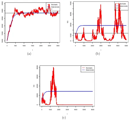
The computer simulations in Figure 5.1 support these results clearly, showing fluctuation around the level 1.2179.
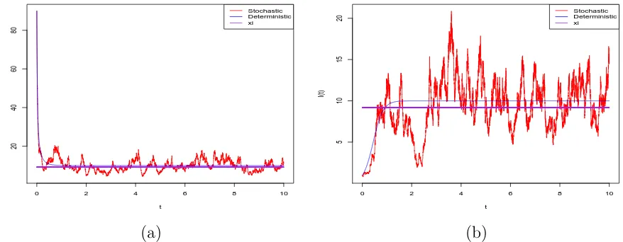
Example 5.3 To further illustrate the effect of the noise intensity σ on the SDE SIS
model, we keep all the parameters in Example 5.2 unchanged but reduce σ to σ = 0.01,
namely we have
β = 0.5, N = 100, µ = 20, γ= 25, σ= 0.01.
So the SDE SIS model (2.4) now becomes
0 2 4 6 8 10
0
20
40
60
80
t
I(t)
Stochastic Deterministic xi
(a)
0 2 4 6 8 10
0
10
20
30
40
t
I(t)
Stochastic Deterministic xi
[image:14.612.80.518.82.253.2](b)
Figure 5.1: Computer simulation of the pathI(t) for the SDE SIS model (5.17) and its
corresponding deterministic SIS model (4.8), using the EM method with step size ∆ = 0.001
and initial values (a)I(0) = 90 and (b)I(0) = 1.
Noting that
R0S = βN
µ+γ −
σ2N2
2(µ+γ) =
50
45−0.011>1,
we compute
ξ= 1
σ2
p
β2−2σ2(µ+γ)−(β−σ2N)= 9.1751.
We can therefore conclude, by Theorem 5.1, that for any initial valueI(0) =I0 ∈(0,100),
the solution of (5.18) obeys
lim inf
t→∞ I(t)≤9.1751 ≤lim supt→∞ I(t) a.s.
The computer simulations in Figure 5.2 support these results clearly, illustrating
persis-tence and that the effect of reducing the standard deviation σ is to increase the level ξ,
which becomes closer to the limiting value of the corresponding deterministic SIS model.
These computer simulations indicate strongly that ξ will increase to N(1−(1/RD
0 )),
which is the equilibrium state of the deterministic SIS model (1.1), as the noise intensity
σ decreases to zero. This is of course not surprising. The following proposition describes
this situation rigorously:
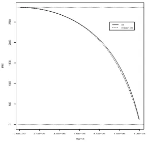
Proposition 5.4 Assume that RS
0 >1 and regard ξ defined by (5.4) as a function of σ
for
0< σ < p
2(βN −µ−γ)
N := ˆσ.
Then ξ is strictly decreasing and
lim
σ→0ξ=N
1− 1
RD
0
and lim
σ→σˆξ =
(
0, if 1≤RD0 ≤2,
NRD0−2 RD
0−1
0 2 4 6 8 10
20
40
60
80
t
I(t)
Stochastic Deterministic xi
(a)
0 2 4 6 8 10
5
10
15
20
t
I(t)
Stochastic Deterministic xi
[image:15.612.79.518.83.254.2](b)
Figure 5.2: Computer simulation of the pathI(t) for the SDE SIS model (5.18) and its
corresponding deterministic SIS model (4.8), using the EM method with step size ∆ = 0.001
and initial values (a)I(0) = 90 and (b)I(0) = 1.
Proof. Compute
dξ
dσ =
1 2
β2
σ4 −
2(µ+γ)
σ2
−12
− 4β
2
σ5 +
4(µ+γ)
σ3
+ 2β
σ3,
= −2β
2+ 2σ2(µ+γ) + 2βp
β2−2σ2(µ+γ)
σ3pβ2−2σ2(µ+γ) ,
= −(
p
β2−2σ2(µ+γ)−β)2
σ3pβ2−2σ2(µ+γ) .
Since σ > 0 we have pβ2−2σ2(µ+γ)−β 6= 0. We therefore have that dξ
dσ < 0
which implies that ξ is strictly decreasing as σ increases. Moreover, by the well-known
L’Hopital’s rule,
lim
σ→0ξ = limσ→0[−(β
2 −2σ2(µ+γ))−1
2(µ+γ) +N] =−µ+γ
β +N =N
1− 1
RD
0
as desired. Furthermore, it is obvious that
lim
σ→ˆσξ =
p
β2−2ˆσ2(µ+γ)−β+ ˆσ2N
ˆ
σ2 .
The numerator equals
|βN −2(µ+γ)|
N +
βN −2(µ+γ)
N ,
so if 1 ≤ R0D ≤ 2 we have limσ→σˆξ = 0, but if RD0 > 2 we have limσ→σˆξ = N
RD
0−2
RD
0−1
Note that Proposition 5.4 implies that for RS
0 > 1, ξ lies between the deterministic
equilibrium value (and limiting value)
N
1− 1
RD
0
for I(t) and
max
0, N
1− 1
RD
0 −1
.
If RD0 is large then ξ will be close to but beneath the deterministic equilibrium value for
I(t).
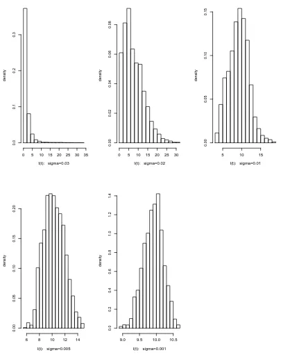
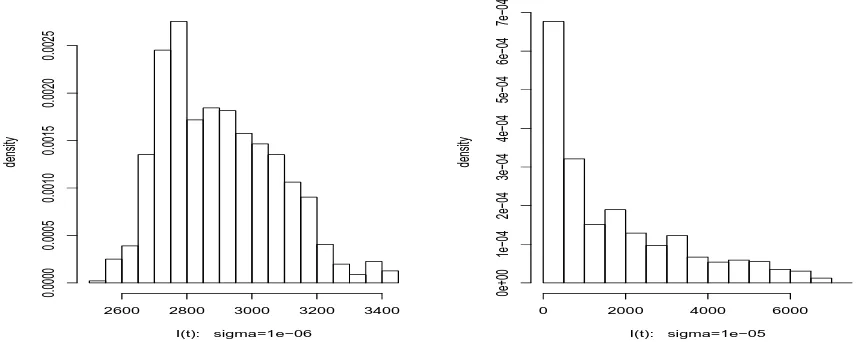
Example 5.5 The computer simulations of the solution to the SDE SIS model in the
persistent case also suggest for higherσ that the distribution of the solution is skewed, as
there are larger oscillations aboveξ than below ξ, while for lower σ the oscillations about
ξ appear to be more symmetrically distributed. This is confirmed by the histograms in
Figure 5.3, showing the distribution ofI(t) in the case ofβ = 0.5, N = 100, µ= 20, γ = 25,
and σ= 0.03, 0.02, 0.01, 0.005 and 0.001, respectively. The simulations were run for
100,000 iterations with step size ∆ = 0.001, i.e. for 100 time steps, and the first 90,000
iterations were discarded to allow for I(t) to reach its recurrent level. The distribution is
positively skewed forσ = 0.03 and 0.02, but asσreduces it becomes more symmetric about
ξ, so that the distribution appears closer to a normal distribution. The corresponding
sample skewness coefficients are 4.8774,0.9319,0.1692,0.1798, and −0.2106.
Testing these data for normality, all tests used were highly significant, conclusively rejecting normality in all cases. This is not surprising in view of the very large sample sizes (10,000), as even moderate deviations from the tested distribution will be significant, however the normal QQ plots in Figure 5.4 suggest that these data are not far from being
normally distributed for smaller values of σ.
6
Stationary Distribution
In the previous section we showed thatI(t) will fluctuate around the level ξ∈(0, N) with
probability 1 when RS
0 > 1. The computer simulations also strongly indicate that the
SDE SIS model (2.4) has a stationary distribution. To be more precise, let PI0,t(·) denote
the probability measure induced by I(t) with initial value I(0) =I0, that is
PI0,t(A) =P(I(t)∈A), A∈ B(0, N),
where B(0, N) is the σ-algebra of all the Borel sets A ⊂ (0, N). If there is a probability
measureP∞(·) on the measurable space ((0, N),B(0, N)) such that
PI0,t(·)→P∞(·) in distribution for any I0 ∈(0, N),
we then say that the SDE (2.4) has a stationary distribution P∞(·) (see e.g. [13, 26]).
I(t): sigma=0.03
density
0 5 10 15 20 25 30 35
0.0
0.1
0.2
0.3
I(t): sigma=0.02
density
0 5 10 15 20 25 30
0.00
0.02
0.04
0.06
0.08
I(t): sigma=0.01
density
5 10 15
0.00
0.05
0.10
0.15
I(t): sigma=0.005
density
6 8 10 12 14
0.00
0.05
0.10
0.15
0.20
I(t): sigma=0.001
density
9.0 9.5 10.0 10.5
0.0
0.2
0.4
0.6
0.8
1.0
1.2
[image:17.612.84.489.66.577.2]1.4
Figure 5.3: Histograms of the values of the pathI(t) for the recurrent SDE SIS model (2.4),
for parameter valuesβ= 0.5, N = 100, µ= 20, γ = 25,I(0) = 90, and differing values ofσ=
0.03, 0.02, 0.01, 0.005 and 0.001.
Lemma 6.1 The SDE SIS model (2.4) has a unique stationary distribution if there is a strictly proper sub-interval (a, b) of (0, N) such that E(τ)<∞ for all I0 ∈(0, a]∪[b, N),
where