Uniform bounds on the 1-norm of the inverse of lower triangular Toeplitz matrices

(1)

bounds on the 1-norm of the inverse of lower triangular Toeplitz

matrices. Linear Algebra and its Applications, 435 (1). pp. 1157-1170.

ISSN 0024-3795 , http://dx.doi.org/10.1016/j.laa.2011.02.044

This version is available at

https://strathprints.strath.ac.uk/30711/

Strathprints

is designed to allow users to access the research output of the University of

Strathclyde. Unless otherwise explicitly stated on the manuscript, Copyright © and Moral Rights

for the papers on this site are retained by the individual authors and/or other copyright owners.

Please check the manuscript for details of any other licences that may have been applied. You

may not engage in further distribution of the material for any profitmaking activities or any

commercial gain. You may freely distribute both the url (

https://strathprints.strath.ac.uk/

) and the

content of this paper for research or private study, educational, or not-for-profit purposes without

prior permission or charge.

Any correspondence concerning this service should be sent to the Strathprints administrator:

[email protected]

The Strathprints institutional repository (https://strathprints.strath.ac.uk) is a digital archive of University of Strathclyde research outputs. It has been developed to disseminate open access research outputs, expose data about those outputs, and enable the

(2)

Contents lists available atScienceDirect

Linear Algebra and its Applications

journal homepage:w w w . e l s e v i e r . c o m / l o c a t e / l a a

Uniform bounds on the 1-norm of the inverse of lower

triangular Toeplitz matrices

<

X. Liu

a

, S. McKee

b

, J.Y. Yuan

c,

∗

_{, Y.X. Yuan}

a

a_{Institute of Computational Mathematics and Scientific/Engineering Computing, AMSS, CAS, Beijing 100190, China} b_{Department of Mathematics, University of Strathclyde, 26 Richmond Street, Glasgow G1 1XH, UK}

c_{Departamento de Matemática – UFPR, Centro Politénico, CP: 19.081, 81531-980 Curitiba, Brazil}

A R T I C L E I N F O A B S T R A C T

Article history:

Received 7 September 2010 Accepted 21 February 2011 Available online xxxx

Submitted by C.K. Li

AMS classification:

15A09 39A10 61A45 65R20 34K28 47B35 74B10 34K06 90C33 15A57 15A0

Keywords:

1-Norm uniform upper bound

Inverse of lower triangular Toeplitz matrix Brunner’s conjecture

Abel equation

A uniform bound on the 1-norm is given for the inverse of a lower triangular Toeplitz matrix with non-negative monotonically decreas-ing entries whose limit is zero. The new bound is sharp under cer-tain specified constraints. This result is then employed to throw light upon a long standing open problem posed by Brunner concerning the convergence of the one-point collocation method for the Abel equa-tion. In addition, the recent conjecture of Gauthier et al. is proved.

<_{The work of the last second authors was supported by the CAPES, CNPq, Fundação Araucária, Brazil, NSFC and CAS, China.}

∗_{Corresponding author.}

(3)

1. Introduction

Consider the Abel equation

t

0

(

t

−

s

)

−α_y

₍

_s

₎

_ds

=

g

(

t

),

t

∈

I

:= [

0

,

T

]

,

(1.1)

withg

(

0

)

₌

0, and

α

_{∈ [}

0

,

1

)

. Its unique solutiony

_∈

C

(

I

)

is given by

y

(

t

)

=

1

γ

α

t

0

(

t

−

s

)

α−1_g′

₍

_s

₎

_ds

_,

_t

_∈

_I

with

γ

α

:=

Γ

(α)

Γ

(

1

−

α)

. Consider its associated difference equation

a0

(

c

;

α)

yi+1

+

i−1

j=0

ai−j

(

c

;

α)

yj+1

=

bi

(

c

;

α),

i

=

0

,

1

, . . . ,

n

,

(1.2)

where the parameterclies in

(

0

,

1

_]

, and the coefficients are given by

(

a

)

a0

(

c

;

α)

=

c

0

(

c

−

s

)

−α_ds

;

(

b

)

ak

(

c

;

α)

=

1

0

(

c

₊

k

₋

s

)

−αds

,

k

₌

1

,

2

, . . . ,

n

_;

(

c

)

bi

(

c

;

α)

=

hα−1g

(

ti

+

ch

),

i

=

0

,

1

, . . . ,

n

.

(1.3)

Here we define ℓ

j=k

≡

0 if

ℓ <

k.

The pointstibelong to a uniform meshIi

= {

ti

=

ih

:

i

=

0

,

1

, . . . ,

n

+

1

;

tn+1

=

T

}

.

This is a collocation method with a single collocation pointti+cper sub-interval

[

ti

,

ti+1

]

.

Note that the casec

₌

1 gives rise to the implicit Euler product-integration method (see e.g. Weiss and Anderssen [14], Eggermont [7]).

In [3] Brunner posed the problem:

Problem 1.1. Given

α

∈ [

0

,

1

)

, for which values ofc

=

c

(α)

∈

(

0

,

1

]

do the solutionsyi+1of the

difference equation (1.2) remain uniformly bounded asn

_{→ ∞}

,

h

_→

0 with

(

n

₊

1

)

h

₌

T?

By evaluating the integrals in (a) and (b) of (1.3) the totality of the difference equations (1.2) may be written as

Tny

=

⎛

⎜ ⎜ ⎜ ⎜ ⎜ ⎜ ⎜ ⎜ ⎜ ⎜ ⎜ ⎜ ⎜ ⎝

c1−α

O

(

1

₊

c

)

1−α

₋

c1−α c1−α

(

2

₊

c

)

1−α

₋

(

1

₊

c

)

1−α

(

1

₊

c

)

1−α

₋

c1−α c1−α

..

. .

.

(

n

+

c

)

1−α

−

(

n

−

1

+

c

)

1−α

. . .

c1−α

⎞

⎟ ⎟ ⎟ ⎟ ⎟ ⎟ ⎟ ⎟ ⎟ ⎟ ⎟ ⎟ ⎟ ⎠

y

₌

d

,

(1.4)

where

y

₌

(

y1

, . . . ,

yn+1

)

T

,

d

=

(

d1

, . . . ,

dn+1

)

T

.

(4)

We note thatTnis a Toeplitz matrix.

Furthermore, in the case of this class of lower triangular Toeplitz matricesTnwe have that

Tn

1

=

Tn

∞

,

due to the fact that

max i

n+1

j=1

|

tij

| =

max j

n+1

i=1

|

tij

|

.

It is easy to see that

T_n−1

1

(

=

Tn−1

∞

)

being uniformly bounded is a necessary condition fory

to remain uniformly bounded. Notice that if

α

₌

0 in (1.1), then the complete answer to Problem 1.1 is known: the solutions of the difference equation (1.2) remain uniformly bounded if, and only

if,c

≥

1

2 (cf. Brunner [3–5]). For 0

< α <

1 is a sufficient condition for uniform boundedness is

c

_≥

c∗

(α)

_:=

₁

2

[

α(

1

₋

α)γ

α

]

1/(1−α)(see [3]). For example,c∗

(α)

≃

0

.

3084 when

α

=

1 2

.

The following conjecture suggests the existence of an upper bound on the inverse of a Toeplitz matrix with a similar, but different structure to that of (1.4).

1.1. GKM conjecture

IfTn

∈

R

(n+1)×(n+1)is the lower triangular Toeplitz matrix whose first column is

1

√

2

(

1

,

√

3

−

1

,

√

5

−

√

3

, . . . ,

√

2n

+

1

−

√

2n

−

1

)

T

,

(1.5)

then for alln,

T_n−1

1

<

3.

Recently, Gauthier et al. [8] proved that an algorithm due to Chen and Mangasarian [6] for solving a mixed linear complementarity problem arising from the discretization of a special system of singular Volterra integral equations would converge if the above conjecture were true.

These and related problems have a long history dating back to the work of Holyhead [10], Weiss and Anderssen [14] and others; yet they appear to have evaded resolution.

Essentially the problem may be regarded as requiring that the 1-norm of the inverse of the lower triangular Toeplitz matrix with specific constraints on its elements be uniformly bounded with respect to its order. Consider the lower triangular

(

n

₊

1

)

_×

(

n

₊

1

)

Toeplitz matrix

Tn

=

⎛

⎜ ⎜ ⎜ ⎜ ⎜ ⎜ ⎜ ⎜ ⎜ ⎜ ⎝

b0

b1 b0

b2 b1 b0

..

.

..

.

. .

.

. .

.

bn

. . . .

b1 b0

⎞

⎟ ⎟ ⎟ ⎟ ⎟ ⎟ ⎟ ⎟ ⎟ ⎟ ⎠

,

(1.6)

which may be characterized by its first column

(

b0

,

b1

, . . . ,

bn

)

Twhereb0

≥

b1

≥ · · · ≥

bn

≥

b

≥

0. The upper bounds for

T_n−1

∞given in [1,12] (see Section2) are not uniform with respect ton

(5)

This paper will be organized as follows. In Section2, a uniform bound is given for the 1-norm of the inverse of the lower triangular Toeplitz matrix (1.6) subject to certain constraints on its elements. Under these restrictions, it is shown that this new bound is sharp. The GKM conjecture is proved in Section3. In the last section, Brunner’s one-point collocation problem is also partially answered. Furthermore, we prove that the 1-norm of Brunner’s associatedTnmatrix is not uniformly bounded when

α

₌

0.

2. Uniform upper bound

Interesting results have already been obtained for matrices of the type defined by (1.6): the main result is given below.

Theorem([1,12] See, also the more recent papers [2,13]). An upper bound on

T_n−1

_∞is given by

T_n−1

_∞

_≤

⎧ ⎪ ⎨

⎪ ⎩

2

b

1

₋

1

₋

_bb

0

[n₂]+1

,

if b

>

0

,

2

b0

_n

2

+

1

,

if b

₌

0

.

(2.1)

In particular if b

>

0,

T_n−1

_∞

_≤

2 b

independently of n and b0.

Note from (2.1) that the upper bound is dependent onnwhenb

₌

0. The GKM conjecture and Problem 1.1 both involve the case ofb

=

0. However, numerical tests clearly show that

T_n−1

∞is

bounded independently ofn. Thus, this paper will deal with obtaining a uniform bound forT_n−1in the 1-norm (or

_∞

-norm) whenb

₌

0 subject to specified constraints on the elements ofTn.

The following lemma, due to Jurkat [11], is an extension of a result by Hardy [9] on inclusion theorems for Norlund means. For clarity and completeness we include Jurkat’s concise proof.

Lemma 2.1. If aiand bisatisfy the conditions

bi

>

0

,

i

=

0

,

1

,

2

, . . . ,

bi+1 bi

≥

bi

bi−1

,

i

₌

1

,

2

, . . .

(2.2)

and

ai

bi

≥

ai−1 bi−1

,

i

₌

1

,

2

, . . . ,

with a0

>

0

,

(2.3)

then all the coefficients, kn, of the Taylor expansion of

∞

i=0 aixi

_∞

i=0

bixi (2.4)

are non-negative. Furthermore, these coefficients of the Taylor expansion are all positive if (2.3) holds as a strict inequality for all i

₌

1

,

2

, . . .

Proof. We first note that n

ν=0

kνbn−ν

=

an forn

≥

0

,

(2.5)

(6)

and

k0

=

a0

/

b0

≥

0

.

(2.6)

Assume thatk1

, . . . ,

kn−1

≥

0. Then we have to show thatkn

≥

0. From (2.5) we have the identity

n−1

ν=0 kν

bn−ν

bn

−

bn−1−ν

bn−1

+

kn

b0 bn

=

an

bn

−

an−1 bn−1

,

(2.7)

and from (2.2)

bn−ν

bn

−

bn−1−ν

bn−1

⎧ ⎨

⎩

=

0

,

for

ν

=

0

,

≤

0

,

for 1

_≤

ν

_≤

n

₋

1

.

(2.8)

Substituting (2.8) into (2.7) and using (2.3), it follows that

kn

b0 bn

≥

an

bn

−

an−1 bn−1

≥

0

.

In a similar way, we can show that these coefficients are strictly positive if (2.3) holds as a strict inequality for alli

=

1

,

2

, . . .

Corollary 2.1. Let bi

,

i

=

0

,

1

,

2

, ...

, be a positive sequence such that

bi+1 bi

,

i

=

0

,

1

,

2

, ....

, is

non-decreasing, then all the coefficients of the Taylor expansion of

1

∞

i=0bixi

(2.9)

are non-positive except the constant term. Furthermore, all these coefficients except the constant term are

negative ifbi+1 bi

,

i

₌

0

,

1

,

2

, ....

, is strictly increasing for all i

₌

0

,

1

,

2

, ...

Proof. It is easy to see that

1

∞

i=0bixi

=

1

b0

−

x b0

∞

i=0bi+1xi

∞

i=0bixi

.

(2.10)

This relation and the previous lemma withai

=

bi+1imply that the corollary is true.

Now we come to a more general case.

Corollary 2.2. Let bi

,

i

=

0

,

1

,

2

, ...

, be a positive sequence such that

bi+1 bi

,

i

₌

2

,

3

, ...

, is

non-decreasing and that the relation

b2 b1

<

b1

b0

≤

b3 b2

(2.11)

(7)

Proof. Again the following identity holds:

1

∞

i=0bixi

=

1

b0

1

₋

γ

1x

−

γ

2x2

−

x3

∞

i=0aixi

∞

i=0bixi

,

(2.12)

where

γ

1

=

b1

b0

, γ

2

=

γ

1

_b2

b1

−

b1 b0

,

(2.13)

and

ai

=

bi+3

−

γ

1bi+2

−

γ

2bi+1

,

(2.14)

for alli

₌

0

,

1

,

2

, ...

. Assumption (2.11) implies that

γ

2

<

0. Consequently, it follows from relation

(2.14) that

ai

≥

bi+3

−

γ

1bi+2

=

bi+2

bi+3 bi+2

−

b1 b0

≥

bi+2

_b

3 b2

−

b1 b0

≥

0

,

(2.15)

for alli

₌

0

,

1

,

2

, ...

. Moreover, we have

ai+1

=

bi+4

−

γ

1bi+3

−

γ

2bi+2

=

bi+3 bi+4 bi+3

−

γ

1bi+3

−

γ

2bi+2

≥

bi+3

bi+2

[

bi+3

−

γ

1bi+2

] −

γ

2bi+2

≥

bi+2

bi+1

[

bi+3

−

γ

1bi+2

] −

γ

2bi+2

=

bi+2

bi+1

[

bi+3

−

γ

1bi+2

−

γ

2bi+1

]

=

bi+2

bi+1 ai

≥

bi+1

bi

ai

,

(2.16)

for alli

=

0

,

1

,

2

, ...

.

We have demonstrated that, in (2.15),

ai

≥

0

,

i

=

0

,

1

,

2

, . . .

(2.17)

and, in (2.16),

ai+1

≥

bi+1

bi

ai

,

i

=

0

,

1

,

2

, . . .

(2.18)

Thus, we may appeal to (2.7) in Lemma 2.1 to show that the coefficients of the Taylor expansion of

∞

i=0aix

i

∞

i=0bix

i

(8)

in (2.12) are all non-negative, and consequently that the coefficients of the Taylor expansion of (2.9) are all non-positive.

We may note that a consequence of this corollary is that

bi+3

−

γ

1bi+2

−

γ

2bi+1

≥

0

,

i

=

0

,

1

,

2

, . . .

(2.19)

We now impose an additional condition on the sequence

_{

bi

}

and provide an estimate of the sum of the coefficients of the Taylor expansion of (2.9).

Lemma 2.2. Suppose that the sequence bi

,

i

=

0

,

1

,

2

, . . .

, satisfies the conditions of Corollary 2.2 and

suppose that

bi+1 bi

≤

1

,

i

₌

0

,

1

,

2

, . . .

(2.20)

Then,

φ (

x

)

=

∞1

i=0bixi

=

1

b0

[

1

−

γ

1x

−

γ

2x2

] −

x3

∞

i=0

θ

ixi

,

(2.21)

where

γ

1and

γ

2are given by (2.13), and

θ

i

≥

0for all i

=

0

,

1

,

2

, . . .

Furthermore, we have that

1

b0

[

1

₋

γ

1

−

γ

2

] −

β

=

∞

i=0

θ

i

,

(2.22)

where

β

₌

⎧ ⎨

⎩

0

,

if ∞

i=0bi

= ∞;

1 ∞

i=0bi

,

otherwise

.

(2.23)

Proof. From Corollary 2.2, (2.21) gives the Taylor expansion of

φ (

x

)

. Due to the assumption (2.20), it follows thatbi

≤

b0for alli

≥

0. Thus, for any given

δ

∈

(

0

,

1

)

, the sequence∞i=0bixiis uniformly convergent on the interval

|

x

| ≤

δ

. Hence, we see that the relation (2.21) holds for all

|

x

|

<

1. Now (2.22) follows from (2.21) by lettingx

_→

1₋. This completes the proof.

Now, we apply the above results to provide an estimate of the 1-norm of lower triangular Toeplitz matrices. First, we can write the matrixTngiven in (1.6) in the following form:

Tn

=

b0I

+

n

i=1

biJi

=

b0I

+

∞

i=1

biJi

,

(2.24)

whereJis the Jordan matrix

J

₌

⎛

⎜ ⎜ ⎜ ⎜ ⎜ ⎜ ⎜ ⎜ ⎜ ⎜ ⎜ ⎜ ⎜ ⎝

0 0 0

· · ·

0 0 1 0 0

_{· · ·}

0 0

0 1 0

· · ·

0 0 0 0 1

_{· · ·}

0 0

..

.

..

.

..

.

. .

.

..

.

..

.

0 0 0

_{· · ·}

1 0

⎞

⎟ ⎟ ⎟ ⎟ ⎟ ⎟ ⎟ ⎟ ⎟ ⎟ ⎟ ⎟ ⎟ ⎠

∈

R

(n+1)×(n+1)

,

(2.25)

(9)

Thus, we have that

T_n−1

₌

φ (

J

),

(2.26)

where

φ (

x

)

is defined in (2.21).

The following result follows directly from Corollary 2.1 and Lemma 2.2.

Theorem 2.1. Suppose that Tnis defined by (1.6) with bi

>

0for i

≥

0. If bi+1

/

biis non-decreasing and

bounded above by 1 for i

=

0

,

1

,

2

, . . . ,

we have the bound:

T_n−1

1

≤

2

b0

−

β,

(2.27)

where

β

is defined in (2.23). If, on the other hand, bi

,

i

=

0

,

1

,

2

, . . . ,

is a positive sequence, bi+1

/

bi

(

i

≥

2

)

is non-decreasing and bounded above by 1 and the condition (2.11) holds then

T_n−1

1

≤

2

b0

1

−

b2

b0

+

_b

1 b0

2

−

β.

(2.28)

Proof. Ifbi+1

/

biis non-decreasing and bounded above by 1 fori

=

0

,

1

,

2

, . . . ,

then it follows from Corollary 2.1 that there exists

θ

˜

i

≥

0 such that

1

∞

i=0bix

i

=

1

b0

−

x

∞

i=0

˜

θ

ixi

.

Thus, by a similar argument to Lemma 2.2, we have

∞

i=0

˜

θ

i

=

1

b0

−

β.

(2.29)

Therefore,

T_n−1

1

=

1

b0

+

∞

i=0

| ˜

θ

i

|

=

1

b0

+

₁

b0

−

β

=

2

b0

−

β.

(2.30)

This proves (2.27).

Now we assume thatbi+1

/

bi

(

i

≥

2

)

is non-decreasing (and bounded above by 1) and, additionally, that the condition (2.11) is satisfied. In this case, we also have the relation (2.29). The assumptions on the sequence

_{

bi

,

i

=

0

,

1

,

2

, . . .

}

and Corollary 2.2 imply that

γ

1

≥

0

, γ

2

≤

0 and

θ

i

≥

0 for all

i

≥

0. Therefore, it follows that

T_n−1

1

=

1

b0

[

1

_{+ |}

γ

1

| + |

γ

2

|] +

∞

i=0

|

θ

i

|

=

1

b0

[

1

₊

γ

1

+ |

γ

2

|] +

∞

i=0

θ

i

=

2

b0

(

1

_{+ |}

γ

2

|

)

−

β.

(2.31)

Since it is clear that

γ

2

<

0, the above equality and (2.13) yield (2.28).

(10)

Note that the bound given in Theorem 2.1 depends onb0

,

b1, andb2but not onn. Consequently it is a uniform bound with respect ton.

3. GKM conjecture

Since the GKM conjecture is relatively straightforward to demonstrate, we shall deal with it first. Using the results given in the previous section, we can easily prove that this conjecture is true.

Theorem 3.1. Let Tn

∈

R

(n+1)×(n+1)be the lower triangular Toeplitz matrix whose first column is given

by (1.5). Then the inequality

T_n−1

1

≤

2

√

2

(

5

₋

√

3

₋

√

5

)

₌

2

.

91860082

<

3 (3.1)

holds for all n

₌

1

,

2

, . . .

Proof.Ifn

₌

1, we have that

T₁−1

1

=

√

2

⎛

⎝

1 0

−

(

√

3

₋

1

)

1

⎞

⎠

1

=

√

2

_[

(

√

3

₋

1

)

₊

1

_]

<

2

√

2

(

5

₋

√

3

₋

√

5

),

(3.2)

which shows that (3.1) holds forn

₌

1. Similarly, direct calculations then provide

T₂−1

1

=

√

2

⎛

⎜ ⎜ ⎜ ⎝

1 0 0

−

(

√

3

₋

1

)

1 0

4

₋

√

3

₋

√

5

₋

(

√

3

₋

1

)

1

⎞

⎟ ⎟ ⎟ ⎠

1

=

√

2

_[

1

₊

(

√

3

₋

1

)

₊

(

4

₋

√

3

₋

√

5

)

_]

=

√

2

(

4

₋

√

5

) <

2

√

2

(

5

₋

√

3

₋

√

5

),

(3.3)

which demonstrates that (3.1) holds forn

=

2 as well.

Now we consider the case whenn

_≥

3. Define the sequencebi

,

i

=

0

,

1

,

2

, . . . ,

as follows:

b0

=

√

1

2

,

bi

=

√

2i

₊

1

₋

√

2i

₋

1

√

2

,

i

=

1

,

2

, . . .

(3.4)

We can easily check that all the conditions forbigiven in Lemma 2.2 (and, consequently, those given in Corollary 2.2) are satisfied. It follows from (2.13) and (3.4) that

γ

2

=

b2 b0

−

_b

1 b0

2

=

√

5

−

√

3

−

(

√

3

−

1

)

2

=

√

5

+

√

3

−

4

.

(3.5)

Moreover, (3.4) also gives

β

₌

0. Thus, from Theorem 21, we have that

T_n−1

1

≤

2

√

2

(

1

_{+ |}

√

5

₊

√

3

₋

4

_|

)

₌

2

√

2

(

5

₋

√

3

₋

√

5

) <

3

.

(3.6)

(11)

4. Brunner’s one-point collocation problem

Consider first the lower triangular Toeplitz matrixTnwhose first column is

(

1

,

21−α

₋

1

,

31−α

₋

21−α

, . . . , (

n

₊

1

)

1−α

₋

n1−α

)

T

,

(4.1)

where

α

_∈

(

0

,

1

)

. This corresponds to the casec

₌

1, which is the case of the implicit Euler product-integration method applied to the Abel equation. Define the corresponding sequence

b0

=

1

,

bi

=

(

i

+

1

)

1−α

−

i1−α

,

i

=

1

,

2

, . . .

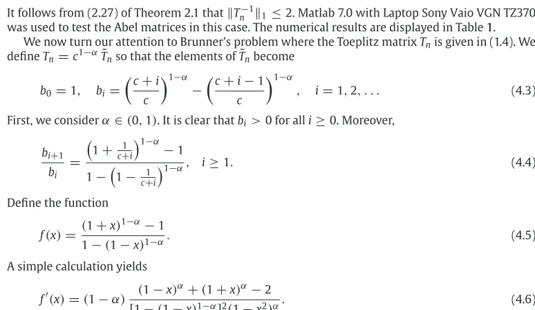
(4.2)

It follows from (2.27) of Theorem 2.1 that

T_n−1

1

≤

2. Matlab 7.0 with Laptop Sony Vaio VGN TZ370

was used to test the Abel matrices in this case. The numerical results are displayed in Table1. We now turn our attention to Brunner’s problem where the Toeplitz matrixTnis given in (1.4). We defineTn

=

c1−αT

˜

nso that the elements ofT

˜

nbecome

b0

=

1

,

bi

=

_c

+

_i

c

1−α

−

_c

+

_i

−

₁

c

1−α

,

i

₌

1

,

2

, . . .

(4.3)

First, we consider

α

_∈

(

0

,

1

)

. It is clear thatbi

>

0 for alli

≥

0. Moreover,

bi+1 bi

=

1

+

c+1i

1−α

−

1

−

1

−

c1+i

1−α

,

i

≥

1

.

(4.4)

Define the function

f

(

x

)

₌

(

1

+

x

)

1−α

−

1

₋

(

1

₋

x

)

1−α

.

(4.5)

A simple calculation yields

f′

(

x

)

₌

(

1

₋

α)

(

1

−

x

)

α

+

(

1

₊

x

)

α

₋

2

[

1

₋

(

1

₋

x

)

1−α

_]

2

₍

₁

₋

_x2

₎

α

.

(4.6) It is easy to verify thatf′

(

x

) <

0 for all

α

∈

(

0

,

1

)

andx

∈

(

0

,

1

)

. Therefore, if

α

∈

(

0

,

1

)

andc

>

0, we have thatbi+1

/

bifori

≥

2 is monotonically increasing and converges to 1. In order to apply Theorem 2.1, we have to consider two separate cases.

(Case A) b2

/

b1

≥

b1

/

b0. This inequality reduces to

ψ

1

(α,

c

)

=

₂

+

_c

c

1−α

−

₁

+

_c

c

1−α

−

₁

+

_c

c

1−α

−

1

2

≥

0

.

(4.7)

It follows from (2.27) of Theorem 2.1 that

˜

T_n−1

1

≤

2 so that

T_n−1

1

≤

2

[image:11.468.36.423.163.387.2]

c1−α

.

(4.8)

Table 1

1-Norm of the inverse of the Abel matrices whenc₌1.

n α₌0 α₌0.4 α₌0.5 α₌0.7

50 2 1.9512 1.9091 1.7331

100 2 1.9682 1.9360 1.7838

1000 2 1.9920 1.9799 1.8912

2000 2 1.9947 1.9858 1.9122

2500 2 1.9954 1.9873 1.9179

3500 2 1.9962 1.9892 1.9258

5000 2 1.9970 1.9910 1.9333

(12)

Graph 1. Case A displayingS1in the(c, α)-plane for whichTn−11is uniformly bounded. (ψ1(c, α)=0 – solid line.)

(Case B) b2

b1

<

b1

b0

≤

b3 b2

.

Thus, from Theorem 2.1, we have the following bound

T_n−1

1

≤

2

1

₊

b2₁

₋

b2

cα−1

₌

2 c1−α

2

₊

₁

₊

_c

c

2(1−α)

−

₁

₊

_c

c

1−α

−

₂

₊

_c

c

1−α

.

(4.9)

The inequality (2.11) implies that (4.7) does not hold andb3

/

b2

≥

b1

/

b0. The latter is the following

inequality

(

3

₊

c

)

1−α

₋

(

2

₊

c

)

1−α

(

2

₊

c

)

1−α

₋

₍

₁

₊

_c

₎

1−α

≥

(

1

₊

c

)

1−α

₋

c1−α

.

(4.10)

The above inequality may be written as

ψ

2

(α,

c

)

=

(

3

₊

c

)

1−α

₋

(

2

₊

c

)

1−α

(

2

₊

c

)

1−α

₋

₍

₁

₊

_c

₎

1−α

−

(

1

₊

c

)

1−α

₋

c1−α

≥

0

.

(4.11)

Therefore, from Theorem 2.1, we have the following result.

Theorem 4.2Let Tnbe defined in(1.4).Then we have that

T_n−1

1

≤

2

(13)

Graph 2. Case B displaying the (small) regionS2in the(c, α)-plane for whichTn−11is uniformly bounded. (ψ1(c, α)=0 – solid line;ψ2(c, α)=0 – dashed line.)

if(4.7)holds.If,however, (4.7)is not satisfied (i.e.

ψ

1

(α,

c

) <

0

)

,then we have that

T_n−1

1

≤

2

c1−α

2

₊

₁

+

_c

c

2(1−α)

−

₁

+

_c

c

1−α

−

₂

+

_c

c

1−α

,

(4.13)

provided that

α

and c satisfy

ψ

2

(α,

c

)

≥

0.

Proof. If (4.7) holds, it follows from (2.27) in Theorem 2.1 that (4.12) is satisfied. If, however, (4.7) does not hold but the inequality (4.11) does, it follows from Theorem 2.1 that (2.28) is satisfied. The bound (2.28) and the form of the elements (4.3) then imply (4.13).

Thus, by plotting the curves

ψ

i

(α,

c

)

=

0

,

i

=

1

,

2, we can easily see the region of

{

(α,

c

)

}

for which

T_n−1

1is uniformly bounded. Indeed,

Tn−1

1 is bounded uniformly for alln, if

(α,

c

)

is

contained within the following two regions:

S1

= {

(α,

c

)

|

ψ

1

(α,

c

)

≥

0

, α

∈

(

0

,

1

),

c

∈

(

0

,

1

]

.

}

(4.14)

S2

= {

(α,

c

)

|

ψ

1

(α,

c

) <

0

, ψ

2

(α,

c

)

≥

0

, α

∈

(

0

,

1

),

c

∈

(

0

,

1

]

.

}

(4.15)

Thus, for any point inS1orS2,

T_n−1

1is bounded uniformly with respect ton.

Three graphs are displayed below. Graph1corresponds to case A while Graph2corresponds to case B. The regionS1for which

Tn−1

1is uniformly bounded is the shaded region in Graph1. The region S2in Graph 2 is extremely small and so a “close-up” (Graph3) is provided:S2is the shaded region in

Graph3.

Finally, we note that in the case

α

=

0, the matrix does not satisfy the conditions of this paper.

(14)

Graph 3. Case B displaying a “close-up” of the regionS2in the(c, α)-plane for whichTn−11is uniformly bounded. (ψ1(c, α)=0 – solid line,ψ2(c, α)=0 – dashed line.)S2is the region defined byψ1(c, α) <0 andψ2(c, α) >0.

However, if

α

₌

0, we have that

Tn

=

cI

+

J

+

J2

+ · · · +

Jn

.

(4.16)

Direct calculations show that

T_n−1

₌

1 c

⎡

⎣I

−

1

c

n

i=1

1

₋

1

c

i−1

Ji

⎤

⎦

.

(4.17)

Thus,

T_n−1

1

=

1

c

⎡

⎣1

+

1

c

n

i=1

! ! ! ! !

1

₋

1

c

i−1!_! ! ! ! ⎤

⎦

=

⎧ ⎪ ⎪ ⎪ ⎪ ⎪ ⎨

⎪ ⎪ ⎪ ⎪ ⎪ ⎩

2

(

2n

₊

1

),

ifc

₌

1

/

2

_;

₁

c

−

1

n

−

2c

c

(

1

−

2c

)

,

1

2

<

c

≤

1

⎫ ⎪ ⎪ ⎪ ⎪ ⎪ ⎬

⎪ ⎪ ⎪ ⎪ ⎪ ⎭

.

(4.18)

Thus, we can conclude that with respect ton,

T_n−1

1is uniformly bounded, ifc

>

1

2

;

and not uniformly bounded, whenc

₌

1

(15)

Acknowledgement

We are grateful to Nick Higham for drawing to our attention the fact that Lemma 2.1 had already been proved by Jurkat [11].

References

[1] K.S. Berenhaut, D.C. Morton, P.T. Fletcher, Bounds for inverses of triangular Toeplitz matrices, SIAM J. Matrix Anal. Appl. 27 (2005) 212–217.

[2] K.S. Berenhaut, R.T. Guy, N.G. Vish, A 1-norm bound for inverses of triangular matrices with monotone entries, Banach J. Math. Anal. 2 (1) (2008) 112–121.

[3] H. Brunner, On systems of Volterra difference equations associated with collocation methods for weakly singular Volterra integral equations, in: S.S. Cheng, S. Elaydi, G. Ladas (Eds.), New Developments in Difference Equations and Applications (Taipei 1997), Amsterdam, Gordon and Breach, 1999, pp. 75–92.

[4] H. Brunner, Discretization of Volterra integral equations with weakly singular kernels, Fields Inst. Commun. 42 (2004) 419–422. [5] H. Brunner, Collocation Methods for Volterra Integral and Related Functional Differential Equations, C.U.P, Cambridge, 2004. [6] C. Chen, O.L. Mangasarian, A class of smooth functions for nonlinear and mixed complementarity problems, Comput. Optim.

Appl. 5 (1996) 97–138.

[7] P.P.B. Eggermont, A new analysis of the trapezoidal-discretization method for the numerical solution of Abel-type integral equations, J. Integral Equations 3 (1981) 317–332.

[8] A. Gauthier, P.A. Knight, S. McKee, The Hertz contact problem, coupled Volterra integral equations, and a linear complementarity problem, J. Comput. Appl. Math. 206 (1) (2007) 322–340.

[9] G.H. Hardy, Divergent Series, Oxford University Press, 1949.

[10] P.A.W. Holyhead, Direct Methods for the Numerical Solution of Volterra Integral Equations of the First Kind, Ph.D. Thesis, University of Southampton, 1976.

[11] W.B. Jurkat, Questions of signs in power series, Proc. Amer. Math. Soc. 5 (6) (1954) 964–970.

[12] A. Vecchio, A bound for the inverse of a lower triangular Toeplitz matrix, SIAM J. Matrix Anal. Appl. 24 (2003) 1167–1174. [13] A. Vecchio, R.K. Mallik, Bounds on the inverses of nonnegative triangular matrices with monotonicity properties, Linear and

Multilinear Algebra 55 (4) (2007) 365–379.

[14] R. Weiss, R.S. Anderssen, A product integration method for a class of singular first kind Volterra equations, Numer. Math. 18 (5) (1972) 442–456.