Detecting Execution Failures Using Learned Action Models
Maria Fox
and
Jonathan Gough
and
Derek Long
Department of Computer and Information Sciences University of Strathclyde, Glasgow, UK
{firstname.lastname}@cis.strath.ac.uk
Abstract
Planners reason with abstracted models of the behaviours they use to construct plans. When plans are turned into the instructions that drive an executive, the real behaviours in-teracting with the unpredictable uncertainties of the environ-ment can lead to failure. One of the challenges for intelligent autonomy is to recognise when the actual execution of a be-haviour has diverged so far from the expected bebe-haviour that it can be considered to be a failure. In this paper we present an approach by which a trace of the execution of a behaviour is monitored by tracking its most likely explanation through a learned model of how the behaviour is normally executed. In this way, possible failures are identified as deviations from common patterns of the execution of the behaviour. We per-form an experiment in which we inject errors into the be-haviour of a robot performing a particular task, and explore how well a learned model of the task can detect where these errors occur.
1
Introduction
In the machine learning literature, methods are described for learning classifications of behaviours based on analy-sis of raw data. These techniques have been applied to in-terpret both human behaviour (Liao, Fox, & Kautz 2004; Ravi et al. 2005; Wilson & Bobick 1999; Nam & Wohn 1996) and robot behaviour (Koenig & Simmons 1996; Fox
et al.2006; Schr¨oteret al.2004). In our earlier work [to be cited] we show that behavioural models can be learned us-ing a fully automated process of abstraction from unlabelled sensor data. These models capture the underlying patterns in the execution of fundamental operations of some execu-tive system. We now show that it is possible to use such a learned model to track a robot while it executes the corre-sponding behaviour in order to follow the evolution of the behaviour at a more abstracted level. This is significant, be-cause it forms a bridge from the primitive sensor level, at which raw data is available, to the abstract level at which a behaviour can be understood symbolically, reasoned about and monitored.
In this paper we show that it is possible to detect when the execution of a behaviour is deviating from its expected course and infer failure in the execution process. As well as recognising that an anomaly has occurred we can pin-point when the failure occurred and attempt a diagnosis of
the failure. This diagnostic capability can be installed on the robotic system, allowing it to track and diagnose its own behaviour. This capability is a prerequisite to automatically recognising plan failure and initiating a replanning effort.
To illustrate this idea with a simple example, consider a robot executing an action of navigating between two points. Suppose the robot has available to it sensors detecting the passage of time and its wheel rotations and a laser sensor al-lowing it to detect distances to objects in line-of-sight. Dur-ing execution of the navigation task the robot can directly observe the values reported by these sensors, but they do not reveal whether the robot is successfully executing the task itself. In order to detect that, the robot must have a model of the process of execution and compare the trajectory of sen-sor readings it perceives with the expectations determined by the model. The key point is that the sensors themselves can never sense failure in the execution — the failure can only be determined by comparing the trajectory seen by the sensors with a model of the behaviour.
The approach we describe is not restricted to monitoring robot behaviour. We are applying the same techniques to learning stochastic models of electrical power transformers based on UHF sensor data. The monitoring approach we describe in this paper is being used to identify, and help di-agnose, changes in the UHF-detectable health states of the transformers.
We begin by summarising the process by which the be-havioural models are learned. We then describe the activity on which we focus in this paper and the data collection strat-egy. We go on to explain the techniques by which we mon-itor execution and, finally, we explore the extent to which these techniques have proven successful.
2
Learning Models of Hidden States
In any physical system there is a gap between its actual oper-ation in the physical world and its state as perceived through its sensors. Sensors provide only a very limited view of re-ality and, even when the readings of different sensors are combined, the resulting window on the real world is still lim-ited by missing information and noisy sensor readings. The consequence is that, in reality, the system moves through
states that arehiddenfrom direct perception. Furthermore,
transi-tions between these hidden states are probabilistic and there is a probabilistic association between states and observa-tions. Such a representation of the behaviour of the system is abstracted from the physical organisation of the device and cannot be reverse-engineered from the control software.
Several authors, including (Ravi et al. 2005; Koenig &
Simmons 1996; Foxet al. 2006), have described methods
for learning abstract behaviour classifications from sensed data. These classifications have been carried out using deci-sion trees, data mining techniques and clustering. In some cases this process was followed by application of the Baum-Welch algorithm to infer a stochastic state transition sys-tem, on a predetermined set of states, to support interpre-tation of the behaviour of the system based on its observa-tions (Koenig & Simmons 1996; Oates, Schmill, & Cohen
2000). Work has also been done to manage theperceptual
aliasingproblem by refining the initial state set (Chrisman
1992). In our work (Fox et al. 2006) we apply a
clus-tering technique to perform the classification of the sensed data into observations. Our approach uses a second cluster-ing step to infer the states of the stochastic model from the observation set, before estimating the underlying stochastic process, so that the whole process of acquiring a behavioural model from raw data is automated.
We make the assumption that the stochastic model can be represented as a finite state probabilistic transition system, so we use Expectation Maximisation (Dempster, Laird, &
Rubin 1977; Baumet al.1970) to estimate a Hidden Markov
Model. Definition 1 describes the structure of the HMM.
Definition 1 A stochastic state transition model is a 5-tuple,
λ= (Ψ, ξ, π, δ, θ), with:
• Ψ ={s1, s2, . . . , sn}, a finite set ofstates;
• ξ={e1, e2, . . . , em}, a finite set ofevidence items;
• π: Ψ→[0,1], the prior probability distributions overΨ;
• δ : Ψ2 → [0,1], the transition model of λ such that δi,j = P rob[qt+1 = sj|qt = si] is the probability of
transitioning from statesi to statesj at time t (qtis the
actual state at timet);
• θ : Ψ×ξ → [0,1], the sensor model of λ such that
θi,k = P rob[ek|si]is the probability of seeing evidence
ekin statesi.
Our objective is to learn HMMs of abstract robot
be-haviours, such asgrasping,moving,recognisingand so on.
Different models must be learned for significantly differ-ent versions of these behaviours (for example, navigating 10 metres in an indoor environment is a very different version of the navigation behaviour from navigating outside). How-ever, a database of models of the key behaviours of the robot can be compiled and used to track its success or failure in the execution of plans.
We claim that, given a model of the successful execution of a given task, subsequent executions can be tracked against
the model and identified as beingexplained by the model, in
which case they are normal, ordivergent from the model, in
which case they can be classed as failing executions. The approach used to explain a sequence of observations with respect to a model is the Viterbi algorithm (Forney 1973).
Our method is to learn how to recognise the normal variabil-ity that exists amongst successful examples of a behaviour, and then to identify significantly divergent examples as ab-normal executions of the behaviour. As we demonstrate be-low, we can also estimate the time at which the divergence occurred, which can help in interpreting the cause of the ab-normality.
An important consequence of having acquired the HMM by a completely automated process is that the states of the transition model have no natural interpretation. We there-fore compare different executions of a behaviour by measur-ing statistical differences between the trajectories that best explain the observation sequences that they produce. This approach relies on the Viterbi algorithm to generate the most probable trajectories but it does not require any understand-ing of the meanunderstand-ings of the states.
3
Experiment
We begin by describing the context in which sensor data was collected, in order to make more concrete the concept of a
trajectorythat we use throughout. We describe the set up here because the first batch of empirical data collection pre-cedes the process of model construction and allows us to better explain the way in which the model can then be used to identify anomalous behaviour.
When a series of observations is generated from sensor readings during an execution of a behaviour, the observa-tions can be fed into the model, using an online implemen-tation of the Viterbi algorithm to find the most likely tra-jectory of states to explain the observation sequence. The sequence can then be assigned a likelihood, which is the probability that the model assigns to the particular trajec-tory it proposes to explain the observation sequence. The se-quence of probabilities generated as more observations are considered will be monotonically decreasing, since longer sequences reside in progressively larger spaces of possible trajectories. For long sequences, these values are very small and will typically underflow the accuracy of floating point representations. As a consequence, we work (as is usual) with log-likelihood measures. We have observed that the pattern of developing log-likelihood across a trajectory falls within an envelope for successful traces, while traces gener-ated by failing executions diverge from the envelope. This occurs because the unusual observations or atypical state transitions made in following the divergent traces have dif-ferent probabilities to those normally followed. As we will see, these probabilities can sometimes be higher than normal and sometimes lower. We discuss this further in the context of some of our results.
Figure 1: The Viterbi sequence probabilities for the training data
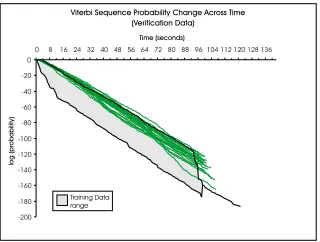
Figure 2: The Viterbi sequence probabilities for the verifica-tion data
while the wheel rotation sensors are reasonably reliable dur-ing straight traverses but tend to be inaccurate durdur-ing turns, when slip and granularity are both problematic. The robot is equipped with a map of its immediate environment which, in the experiment reported here, consisted of a collection of boxes arranged around it.
Our data was collected in a series of batches: 50 training executions, 20 verification executions and 40 error execu-tions, split into four groups of 10 executions for different errors. The training data was used to learn the HMM, and the verification data was kept separate so that the learnt mod-els could be tested. The error data consisted of executions in which a specific type of error was induced. Figures 1 and 2 show the envelope for the log-likelihood values on the training data and the log-likelihood values for the sub-sequent verification data set. There is one execution in the training data that took about twenty seconds longer to com-plete than the rest, and this protrudes past the end of the rest of the data. The most likely reason for this single execution taking longer is a build up of errors that led to a series of localisation steps that did not correct the error entirely.
[image:3.612.359.518.53.173.2]The verification data was collected in an entirely recon-structed environment, rather than simply being a subset of the data collected during training. This helps to explain why the traces in the verification data are not evenly placed within the training envelope and also serves to emphasise the robustness of the learned model. The difference in the verification environment was significant (it was constructed
Figure 3: The Viterbi sequence probabilities for the ‘Lost Connection’ error data
in a different laboratory, with quite different physical dimen-sions and different floor covering), so the fact that the model continues to provide a good characterisation of the under-lying behaviour in this task is a significant validation of its performance.
For all of the error executions, data was collected up to the point that the task finished or long enough to allow a reasonable algorithm to detect an error. The errors induced were as follows:
Lost Connection The radio connection between the con-trolling computer and the robot was disconnected, mean-ing that the robot stopped receivmean-ing commands and could not transmit new sensor data.
Blocked The robot was trapped so that it was unable to turn to the next angle to take a photograph. This is to sim-ulate the robot becoming blocked by some environmental factor.
Slowed In this data, the robot was deliberately slowed down by exerting friction on the top of the robot. This caused the robot to turn much more slowly than normal.
Propped Up This set of data was collected to simulate the robot “bottoming-out” by the wheels losing contact on the ground on an uneven surface. The front of the robot was propped-up on a block so that the wheels could not make the robot rotate. The execution continues as normal as the robot wheel sensors indicate that it is still rotating, however there may be an extreme number of localisation steps as it tries to correct the errors of inconsistency in its sonar readings. Eventually the robot’s localisation cannot keep up with the errors and it becomes highly inaccurate. We now consider the data collected from these failing tra-jectories.
[image:3.612.94.254.218.339.2]Figure 4: The Viterbi sequence probabilities for the ‘Blocked’ error data
as the training data up to a point, and then breaks off before decreasing at the slower rate. The other four cases (fail-ures induced at 6, 12, 24 and 20 seconds) show no obvious changes in the rate of probability decrease, and all appear with probabilities similar to the training data.
It may seem strange at first that in the majority of the fail-ure cases the probabilities are higher than the training data, but this is to be expected. The probability reported by the Viterbi algorithm is the chance that a particular sequence of observations produced a particular output sequence of states. The higher probability that the Viterbi sequence explains the observation sequence is not to be interpreted to mean that
the sequence itself is more likely, but rather thatgiven the
observation sequencethe generated state trajectory is more likely. The panoramic image behaviour (in common with many others) exhibits a regularity of structure that is mod-elled by loops on individual, or sets of, states. With thought it is easy to see that a repeated observation is best explained by a repeated visit to a single state. The HMM seeks out the best state (or states) to repeat in order to maximise the probability of the sequence.
Blocked Errors (Figure 4) As with the error cases in which the connection was terminated, these executions have probabilities that deviate upwards from the training data.
The difference here is thatallof the sequences exhibit this
behaviour, rather than simply the majority. One explanation for this could be that the data reported from the sensors in this case will always indicate that the robot is barely moving, while the lost connection will lead to repetition of whatever sensed data was last detected.
Slowed Errors (Figure 5)Since the robot is being slowed down during turning, the action takes much longer to com-plete than the normal executions. In these error cases, the probabilities decrease at a greater rate than normal,
proceed-ing to a minimum probability of around10−300, compared
to a minimum of10−120for the training data. The very low
probabilities of sequences are due to the fact that the most appropriate HMM sequences in these cases loop on states that have low self-transition probabilities. Such trajectories are highly unlikely to occur.
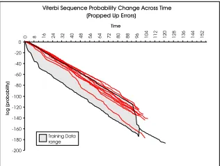
[image:4.612.360.518.53.175.2]Propped Errors (Figure 6)The data collected from these error executions do not show any apparent difference to the training or verification data. The probabilities reported are
Figure 5: The Viterbi sequence probabilities for the
‘Slowed’ error data
Figure 6: The Viterbi sequence probabilities for the
‘Propped Up’ error data
within acceptable limits and it is impossible to distinguish these executions as possessing any anomalies.
4
Automatic Error Detection
We propose two methods for automatic detection of anoma-lous execution traces.
4.1
Cumulative difference
The first method is based on an an approach we call
Cu-mulative Log Probability Difference, or CLPD. The CLPD measures how far the sequence has wandered outside the range defined by the maximum and minimum probabilities seen for the training data. If the sequence wanders outside the boundaries seen for a particular timepoint, the difference between the log probabilities is summed. By definition, the training data always remains in this range and will always have a CLPD of 0.
More formally, with the following:
px = log prob. seq. atx
mx = max log(prob. train data atx)
nx = min log(prob. train data atx)
CLPD is defined:
LP Dx= 0 [nx< px< mx]
(px−nx) [px< nx]
(mx−px) [px> mx]
CLP Dx= x X
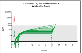
[image:4.612.360.518.218.337.2]Figure 7: The CLPD values for the verification data
Figure 7 shows the CLPD of the verification data, plotted on a log scale vertically for clarity. Note that all but two
of the executions have CLPDs of below 5001, suggesting
that in this task a CLPD of 500 or lower is a good indicator of successful execution. Once a sequence has a CLPD of over 500 it can be identified as having failed.
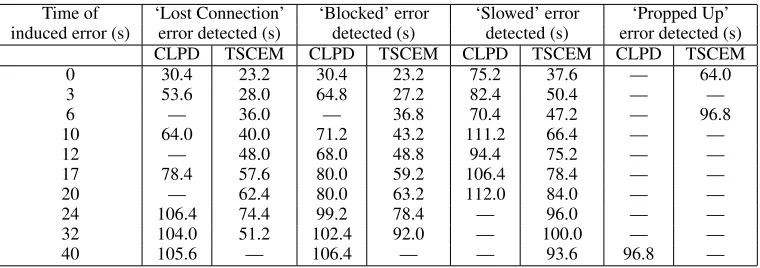
Figure 8 shows the times at which the CLPD value ex-ceeds 500 in each of the anomalous traces. Note that most of the errors in the ‘Lost Connection’, ‘Blocked’ and ‘Slowed’ data were detected before the action terminated, but only one of the ‘Propped Up’ errors was detected. The latter er-ror type is much more difficult to characterise for this robot in terms of a physical behaviour that is different to a normal execution, because of its limited sensory capacity. Indeed, a human presented with the raw data of one of these exe-cutions and a normal execution would be unlikely to distin-guish between the two. It had been hoped that there would be a difference in the amount of localisation required for this error type, but it seems that the sonar data and sub-routines for localisation are not accurate enough to provide meaningful data when such errors occur. Had the robot been equipped with a more accurate localisation device (such as a laser range-finder) as well as a more sophisticated locali-sation algorithm then these errors might have been detected. We intend to explore this hypothesis with a more sophisti-cated robot in the future.
4.2
Temporal state counting
We now consider an alternative approach to anomaly detec-tion. Temporal state counting attempts to identify Viterbi se-quences with an anomalous number of occurrences of states (either too few or too many) in comparison with the numbers of occurrences of states in successful trajectories. To mea-sure the amount of error, a similar technique to the proba-bilistic anomaly detection above is used. The difference be-tween the observed number of occurrences of each state and the expected number of states at each timepoint is summed. This may be formally defined as follows:
c(τ, s, x) = #occs.sto timexfor traceτ
m(s, x) = maxT #sto timex
n(s, x) = minT #sto timex
1
One execution exceeds a CLPD of 500 just before the end of the task, when there was only one training execution of this length. There was little evidence for the possible spread of values at this timepoint causing CLPD to rise sharply after this point. A larger training sample would probably have removed this problem.
Figure 9: The TSCEM values for the verification data.
where “#s” is the number of occurrences of statesin the
states for the corresponding trajectory and the maximum and minimum values (form(s, x)andn(s, x)) are defined of the range of traces inT, the set of all training data.
The error magnitude for statesat timepointxis defined
to be a measure of how far the current execution deviates from the training data:
e(s, x) =
0 [n(s, x)< c(s, x)< m(s, x)]
n(s, x)−c(s, x) [c(s, x)< n(s, x)]
c(s, x)−m(s, x) [c(s, x)> m(s, x)]
Temporal State Count Error Magnitude (TSCEM) for a
sequence at timepointxis defined to be the sum of all error
magnitudes across all states up to that timepoint:
T SCEMx= x X
i=0
t X
s=0 e(s, i)
!
wheretis the number of states in the HMM.
Figure 9 shows the TSCEM values for the verification data. Note that the magnitude of the errors is usually be-low 100, and only one has a TSCEM value of over 125. Be-cause of this, we consider a TSCEM value over 125 as an indication of failure for this task. Figure 8 also shows the performance of our algorithm based on Temporal Anomaly Detection in our examination of the test data. As with Proba-bilistic Anomaly Detection, identification of the ‘Lost Con-nection’, ‘Blocked’ and ‘Slowed’ errors was very success-ful. However, this technique detected the errors more re-liably than the CLPD technique. The technique was less successful with the ‘Propped Up’ errors.
A possible refinement would be to find the distri-bution of occurrences of each state at each timepoint,
rather than simply the maximum and minimum. The
sum of the number of standard deviations by which each statecount varies (Z-score) could be taken instead
of the TSCEM value. This is defined as follows:
µ(s, x) = meanT #sto timex
σ(s, x) = stddevT #sto timex
The normalised error magnitude for statesat timexis then:
N SCEMx= x X
i=0 t X
s=0
c(s, i)−µ(s, i)
σ(s, i)
!
dis-Time of ‘Lost Connection’ ‘Blocked’ error ‘Slowed’ error ‘Propped Up’ induced error (s) error detected (s) detected (s) detected (s) error detected (s)
CLPD TSCEM CLPD TSCEM CLPD TSCEM CLPD TSCEM
0 30.4 23.2 30.4 23.2 75.2 37.6 — 64.0
3 53.6 28.0 64.8 27.2 82.4 50.4 — —
6 — 36.0 — 36.8 70.4 47.2 — 96.8
10 64.0 40.0 71.2 43.2 111.2 66.4 — —
12 — 48.0 68.0 48.8 94.4 75.2 — —
17 78.4 57.6 80.0 59.2 106.4 78.4 — —
20 — 62.4 80.0 63.2 112.0 84.0 — —
24 106.4 74.4 99.2 78.4 — 96.0 — —
32 104.0 51.2 102.4 92.0 — 100.0 — —
[image:6.612.117.497.52.186.2]40 105.6 — 106.4 — — 93.6 96.8 —
Figure 8: Probabilistic and Temporal Anomaly Detection performance across the error data. Time for a successful run was around 100 seconds in the training data and 110 seconds in the verification data.
tributions for each state at each timepoint. This method re-mains a subject for further research.
Using TSCEM we can detect errors earlier, and detect more of them. TSCEM successfully identified 30/40 errors, while CLPD identified only 24/40. The combination of tech-niques, however, is a more reliable test than either test indi-vidually, allowing us to correctly identify 33/40 cases, in-cluding all of the first three types. As commented earlier, we believe that the ‘Propped Up’ error type is hard to find given the nature of the sensors available to this robot.
5
Conclusion
When an executive system is required to turn a plan, con-structed from abstract action models, into execution, while sensing its environments through imperfect sensors, there is no direct way to detect when the execution of an individual action has failed. We have described a controlled experiment in which we confirmed that a model learned from success-ful executions of a particular behaviour could reliably ex-plain subsequent, unseen, successful trajectories, and could also recognise failing trajectories as divergent with high re-liability. We have presented two statistical measures for de-termining that trajectories are divergent. The first, CLPD, measures the extent to which a trajectory has diverged from the envelope of accepted trajectories by considering the ac-cumulation of divergence in the log probability of the given trajectory from the extremes of the envelope. The second, TSCEM, measures the extent to which revisiting the same state causes a trajectory to become divergent (even when the well-explained trajectories also contain state loops).
We have demonstrated that it is possible to use mod-els that bridge the gap between the low-level sensory data streams and the higher level abstract action models to mon-itor execution. In doing so, we are able to detect failures in execution, often anticipating the point at which the action might otherwise have completed execution. The approach we have described is complementary to the use of direct sen-sor interpretation methods and represents a form of model-based reasoning (Williams & Nayak 1996).
The next step in this work is to react to having detected failure by controlling what the robot does next. At this time
we can only detect that failure has probably occurred (even if it is not yet externally visible) and cause the robot to ter-minate its activity. This is a conservative reaction to pre-vent the robot from entering an unsafe state. It would be interesting to react by switching the robot into an alternative behaviour and then continuing to monitor its execution by tracking against the appropriate model. We are considering this possibility in our current work.
Finally, we believe that our approach can be used not only in monitoring the execution of actions for robotic systems, but also to monitor the behaviour of systems, both engi-neered and natural, using models learned from data gath-ered from monitored traces of their behaviours over time. This work is already progressing in application to condition monitoring of electrical plant items and will be reported in future work.
References
Baum, L.; Petrie, T.; Soules, G.; and Weiss, N. 1970. A maximization technique occurring in the statistical analysis of probabilistic functions of Markov chains.Ann. Math. Statist.41(1):164–171. Chrisman, L. 1992. Reinforcement Learning with Perceptual Aliasing. InProceedings of the 10th National Conference on AI (AAAI), 183–188.
Dempster, A. P.; Laird, N. M.; and Rubin, D. B. 1977. Maximum Likelihood from Incomplete Data via the EM algorithm.Journal of the Royal Statistics Society39(1):1–38.
Forney, G. D. 1973. The Viterbi Algorithm.Proceedings of the IEEE61:268–278.
Fox, M.; Ghallab, M.; Infantes, G.; and Long, D. 2006. Robot Introspection through Learned Hidden Markov Models.Artificial Intelligence170(2):59–113.
Koenig, S., and Simmons, R. G. 1996. Unsupervised Learning of Probabilistic Models for Robot Navigation. InProceedings of the International Conference on Robotics and Automation, 2301– 2308.
Liao, L.; Fox, D.; and Kautz, H. 2004. Learning and Inferring Transportation Routines. In
Proceedings of the 19th National Conference on AI (AAAI), 348–354.
Nam, Y., and Wohn, K. 1996. Recognition of Space-Time Hand Gestures using Hidden Markov Models. InACM Symposium on Virtual Reality Software and Technology, 51–58.
Oates, T.; Schmill, M.; and Cohen, P. 2000. A Method for Clustering the Experiences of a Mobile Robot that Accords with Human Judgements. InProceedings of the 17th National Conference on AI (AAAI), 846–851.
Ravi, N.; Dandekar, N.; Mysore, P.; and Littman, M. 2005. Activity recognition from accelerom-eter data. InProc. of 17th Conf. on Innovative Applications of AI (IAAI).
Schr¨oter, D.; Weber, T.; Beetz, M.; and Radig, B. 2004. Detection and classification of gateways for the acquisition of structured robot maps. InProc. 26th Pattern Recognition Symposium. Williams, B. C., and Nayak, P. P. 1996. A Model-based Approach to Adaptive Self-configuring Systems. InProceedings of the 13th National Conference on AI (AAAI), 971–978.
Wilson, A., and Bobick, A. 1999. Parametric Hidden Markov Models for Gesture Recognition.