Development of an experiment-based robust design paradigm for multiple quality characteristics using physical programming

(1)

ORIGINAL ARTICLE

Development of an experiment-based robust design

paradigm for multiple quality characteristics using physical

programming

Jami Kovach&Byung Rae Cho&Jiju Antony

Received: 18 April 2006 / Accepted: 5 September 2006 / Published online: 8 November 2006 #Springer-Verlag London Limited 2006

Abstract The well-known quality improvement methodol-ogy, robust design, is a powerful and cost-effective technique for building quality into the design of products and processes. Although several approaches to robust design have been proposed in the literature, little attention has been given to the development of a flexible robust design model. Specifically, flexibility is needed in order to consider multiple quality characteristics simultaneously, just as customers do when judging products, and to capture design preferences with a reasonable degree of accuracy. Physical programming, a relatively new optimization technique, is an effective tool that can be used to transform design preferences into specific weighted objectives. In this paper, we extend the basic concept of physical program-ming to robust design by establishing the links of experimental design and response surface methodology to address designers’ preferences in a multiresponse robust design paradigm. A numerical example is used to show the proposed procedure and the results obtained are validated through a sensitivity study.

Keywords Multiresponse robust design . Physical programming . Optimization . Flexibility . Preferences . Experimental design . Response surface methodology

1 Introduction

1.1 The design process

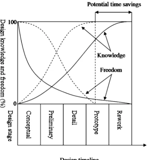
A designer’s main task is to apply scientific knowledge to the solution of technical problems and then to optimize that solution within the given constraints in order to determine the major attributes of the product, such as capability to meet product specifications, quality, and cost. During the early stages of the design process, there are many uncertainties involved in the decision-making process. As a design evolves, more information becomes available, and the designer’s understanding of the situation grows. Figure1 shows the relationship between the design timeline and knowledge about the design, where the solid lines indicate the current measurements regarding the design process. We can observe that knowledge and freedom have an inverse relationship over the course of the design timeline. This relationship is ironic in that the designer has maximum design freedom when the knowledge about the design is minimal, but in the later stages when there is more information available, the designer has very little design freedom. Ideally, the designer should have maximum freedom in the later stages of the design process, when more information concerning the design parameters is available. The dashed lines in Fig. 1 depict the potential time savings that could be achieved by improving design flexibility in the early stages of design. By providing flexibility in design, rework, time to market, and product costs could be reduced. Ways to achieve design flexibility DOI 10.1007/s00170-006-0792-z

DO00792; No of Pages J. Kovach

Department of Information and Logistics Technology, 312 Technology Building, University of Houston, Houston, TX 77204, USA

B. R. Cho (*)

Advanced Quality Engineering Laboratory,

Department of Industrial Engineering, 110 Freeman Hall, Clemson University,

Clemson, SC 29634, USA e-mail: [email protected]

J. Antony

Division of Management, Caledonian Business School, Glasgow Caledonian University,

(2)

include designing to accommodate changes or designing to anticipating changes that might occur. The latter method has proven unsuccessful because uncertainty is involved; therefore, the better solution is to design to accommodate changes with minimal rework cost.

1.2 Literature review

Among the design methods currently studied in engineer-ing, researchers often identify robust design (RD) as one of the most important fields for the purpose of quality improvement. RD, which was first conceptualized by Taguchi [1, 2], is a cost-effective method to determine the optimum operating conditions of a system, using optimization techniques and design of experiments, in order to reduce costs and improve quality. By optimizing the design of products and processes, RD produces high-quality products with low development time and manu-facturing costs. A comprehensive analysis of RD can be found in [3,4].

Taguchi’s greatest contribution to the area of quality engineering was his quality philosophy, which simulta-neously incorporates the mean and variability of a quality measure into product and process design in order to reduce variation. While the basic concept of RD is clearly important, Taguchi’s assumptions, experimental design, and statistical analysis, have drawn much criticism. Com-plete discussions of the merits and deficiencies of Taguchi’s

RD can be found in [5–12]. As a result, there have been many attempts in the literature to integrate Taguchi’s RD principles with established statistical techniques, such as response surface methodology (RSM). RSM is a statistical tool that is useful for modeling and analysis in situations where the response of interest is controlled by several input factors. A comprehensive review of RSM is presented in [13].

Early work in this area by Vining and Myers [14] combines Taguchi’s RD principles with conventional RSM in order to model the response of interest directly as a function of the design factors. This approach is known as the dual response model, where the goal is to minimize the process variance while adjusting the process mean to the desired target value. Further, work by del Castillo and Montgomery [15] and Copeland and Nelson [16] showed that standard nonlinear programming techniques, such as the generalized reduced gradient method and the Nelder-Mead simplex method, may provide more effective RD solutions. It is important to note, however, that the dual response approach does not always guarantee optimal settings of design variables, which are often referred to as design factors, since the approach strictly requires a zero-bias assumption by forcing the process mean to be located at the target value. To address this issue, Cho [17] and Lin and Tu [18] proposed the mean-squared error (MSE) approach by relaxing this zero-bias assumption. This approach shows that, while allowing some process bias, the resulting process variance would be less than or, at most, equal to the variance of the dual response approach; hence, the MSE approach provides better (or at least equal) settings of design factors than previous approaches. Further research in this area has been discussed in the literature [19–24].

Most traditional RD problems, such as those discussed previously, focus on a single-objective optimization ap-proach, which considers only one performance measure. Several attempts have been made in the literature to optimize multiresponse problems in the context of RD. Four well-known methods are: (1) the contour overlay method, which uses visual inspection of superimposed response contour plots, but becomes less practical as the number of design variables increases; (2) the desirability function method (see [25, 26]), which transforms the multiresponse problem into a single-response problem by maximizing the combined desirability; (3) the Khuri and Conlon [27] method, which uses the generalized distance approach to find the optimal settings that minimize the distance function over the experimental region; and (4) the loss function approach (see [28]), which uses a quadratic loss function to solve problems with multiple quality characteristics. Several other attempts have been made to optimize multiresponse problems; however, most of these

[image:2.595.52.292.56.315.2]

(3)

methods are complex and inflexible. Although the RD methods reviewed here are clearly effective, there is room for improvement.

1.3 Research motivation

Most RD models reported in the literature consider a single quality characteristic. However, in most real-world indus-trial settings, multiple quality characteristics are often considered because customers judge products simulta-neously on a variety of scales. Therefore, the objective should be to find the optimal settings for the design variables while considering multiple quality characteristics simultaneously. Yet, a vast majority of RD models fail to consider the implementation of design flexibility by not capturing preferences with a reasonable degree of accuracy. Therefore, most of these RD models involve iterative weight tweaking, as there is no clear method of prioritiza-tion. A physical programming approach to RD has been studied in [29–33]. The main focus of these papers was to improve design flexibility based on the preferences of the designer with the consideration of multiple quality charac-teristics using physical programming. As a further step, we propose a physical programming model for experiment-based RD by integrating the logistics of physical program-ming and experimental design by linking the concept of RSM to a multiresponse RD problem, which has not been fully studied in previous work. The proposed RD model is demonstrated through the use of a numerical example. A sensitivity analysis is also conducted in order to evaluate the effects of various model parameters on the results, which provides practitioners with insights into the practical implementation of the proposed model.

2 Robust design considering multiple objectives

Due to the practicality of multiresponse RD, other work in this area is discussed here for the benefit of the reader. Logothetis and Haigh [34] used multiple regression and linear programming in a two-step approach to address multiresponse problems. Similar to Pignatiello’s approach [28], Elsayed and Chen [35] and Ames et al. [36] also developed a multiple quality characteristic model based on the expected loss function. Derringer [37] further improved his approach to multiresponse problems by proposing a weighted desirability function. Kapur and Cho [38] pro-posed a multiresponse technique based on the criteria of minimizing deviation from the target and maximizing the robustness to noise, where a weighted penalty is incurred if the product characteristics deviate from their target values. An approach based on principal component analysis (PCA) was developed by Su and Tong [39]. Additionally, Tong

and Su [40] utilized fuzzy set theory in weight-setting as an approach to optimize the multiresponse problem. Tong et al. [41] standardized the loss of each quality characteristic of interest so that standardization values ranged between 0 and 1. Chen [42] developed a multiple-quality-characteris-tic-based model where the designer’s degree of satisfaction with each quality characteristic is represented by a transformation of the signal-to-noise ratio to a commensu-rable value between 0 and 1. Kim and Lin [43] suggested a mathematical programming formulation for the dual re-sponse problem based on fuzzy optimization, called the fuzzy modeling approach. The goal is to identify the operating conditions that maximize the minimum degree of satisfaction with respect to the mean and variance within the feasible region. Vining [44] proposed a compromise approach to the multiresponse problem where the analyst can consider process economics and correlation structure. Tsui [45] used the expected loss function derived by Pignatiello [28] and extended this work to create a new model for other types of quality characteristics. Chen et al. [32] and Messac and Ismail-Yahaya [33] utilized physical programming to address the incorporation of designers’ preferences into the multiresponse RD problem. Chiao and Hamada [46] proposed a multiple polynomial regression model to optimize the results of experiments where quality characteristics are correlated. To address the consideration of asymmetric quality loss, Kim and Cho [47] developed a priority-based RD model utilizing both the concepts of the dual response approach and nonlinear goal programming techniques. Based on the same goal programming tech-niques, Tang and Xu [48] proposed a unified formulation for the dual response optimization model by assigning different weights to bias and variability. Lin et al. [49] used fuzzy logic and Lu and Antony [50] used fuzzy-rule-based inference as separate approaches to the multiresponse problem. Romano et al. [51] utilized a total loss criterion, which raises customer satisfaction to the same level of concern as production costs. Wu and Chyu [52] built on Chiao and Hamada’s model [46] by considering the loss coefficient of single characteristics and those between two correlated characteristics. The RD model proposed in this paper attempts to build on previous work in this area to further explore the simultaneous use of physical and goal programming approaches in multiresponse RD problems to better address process design and modeling flexibility issues by establishing links of experimental design to RD.

3 Proposed approach

(4)

knowledge possessed by the designer is exploited in order to impart design flexibility into the RD model for a multiresponse problem. The proposed model consists of the following steps:

1. Identify the design variables and quality characteristics of interest. This is often accomplished by screening experiments or is based on prior knowledge concerning the system under investigation.

2. Design an experiment to examine the chosen system variables and responses. Choose an experimental design that supports the desired analysis.

3. Conduct the experiment. Collect the specified data for each experimental trial.

4. Analyze the data. Estimate the fitted functions for the mean and variance of each quality characteristic using RSM.

5. Classify the mean and variance of each quality characteristic. Categorize the attributes based on the desired behavior of each response.

6. Incorporate preferences. Obtain preferences with re-spect to each quality attribute as specified by the designer and use these preferences to generate weights for use in the optimization model.

7. Build the objective function. Use preference weights and deviation variables to form an aggregate objective function.

8. Determine the optimal process parameter settings.Use the optimization model developed here to obtain the optimum operating conditions.

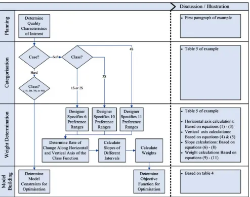
The planning through analysis stages of the proposed model follows the traditional RD method closely, in terms of experimental design and response modeling. However, during experimentation, data are collected for multiple responses, and fitted functions are determined for the mean and variance of each quality characteristic of interest. These equations are then used simultaneously to solve the multi-response problem using the classification method and optimization model proposed in this work. These tech-niques are further developed in the following sections.

3.1 Method of classification

The proposed RD model uses a physical programming framework, but the framework has been customized to fit the particular model under consideration through the incorporation of goal programming techniques. In the proposed model, the estimated response surface functions for the process mean and variance are treated as individual quality attributes. Then, trade-offs between quality charac-teristics are made by allowing the designer to express preferences in a fashion that is less rigid and more flexible than traditional methods. Using the physical programming

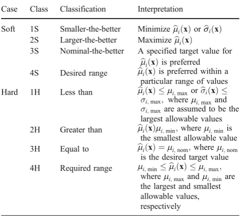
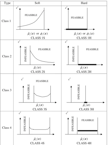
approach, the preferences expressed by the designer are classified into one of four classes, and each class includes two sub-cases (hard and soft cases). Thus, the desired behavior of the mean and variance of each quality characteristic is classified into one of these categories, which are shown in Table 1. Graphical representations of the qualitative meaning of each class are displayed in Table2.

[image:4.595.305.545.497.713.2]

A quality characteristic is classified as a soft class if it has a preferred target value where it needs to be either minimized, maximized, or should fall within a desired range. But, as the name suggests, these requirements are flexible. The mean function of a quality characteristic can be classified into any one of the four classes; however, the standard deviation always belongs to class 1S due to the fact that, in RD, the variance is preferred to be as small as possible. Oppositely, if the preferred value of a quality attribute is not flexible in that it is either feasible or infeasible, then it is classified as a hard class. The hard classes are applicable in situations where the designer must stay within a specified range. The values associated with hard classes are either acceptable or not acceptable; there are no other distinctions in the hard classes. For each response, the designer is asked to express their preferences in detail by specifying different ranges of acceptability. These ranges are based on the designer’s prior knowledge concerning the system under investigation and/or historical data. Then, based on these ranges, a class function is formed which determines how sensitive the solution would be to the design specifications. These functions map the units and physical meaning of each response range to a

Table 1 Definitions of quality characteristic classifications Case Class Classification Interpretation

Soft 1S Smaller-the-better Minimizebmið Þx orbsið Þx 2S Larger-the-better Maximizebmið Þx

3S Nominal-the-better A specified target value for

b

mið Þx is preferred 4S Desired range bmið Þx is preferred within a

particular range of values Hard 1H Less than bmið Þ x mi;maxorσibð Þ x σi;max; wheremi;maxand σi;maxare assumed to be the largest allowable values 2H Greater than bmið Þxmi;min;wheremi;minis

the smallest allowable value 3H Equal to bmið Þ ¼x mi;nom;wheremi;nom

is the desired target value 4H Required range mi;minmbið Þ x mi;max;

(5)

dimensionless scale, which is represented as a unimodal function and guides the path of the optimization process.

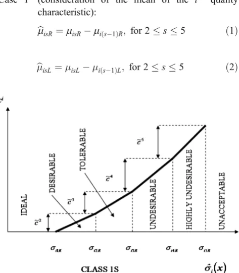
After classifying each of the quality characteristics into one of the four classes, the designer has to specify preferred values based on the extent of preference for each class. For each quality characteristic belonging to classes 1S and 2S, the designer has to specify six ranges of preferred values, while for classes 3S and 4S, ten and eleven ranges are specified, respectively. The six ranges for classes 1S and 2S are defined in Table3. Figure2shows the class function for

the standard deviation of a quality characteristic. Here, we use the notation where xis the set of design variables and the fitted functions of the mean and standard deviation are b

m_ið Þx and bsið Þ;x respectively. The value of the criterion under consideration, sbið Þ;x lies along the horizontal axis, and the class function, ci, is depicted on the vertical axis. Similar diagrams can be created to examine the criterion b

m_ið Þx and/or other classes (see [30]); however, the shape of the class function depends on the numerical values of the range limits for the preferences specified by the designer.

Type

Soft

Hard

Class 1

c

i

)

(

ˆ

x

µ

i

or

σ

ˆ

i

(

x

)

CLASS 1S

c

i

)

(

ˆ

x

µ

i

or

σ

ˆ

i

(

x

)

CLASS 1H

Class 2

c

i

)

(

ˆ

x

µ

i

CLASS 2S

c

i

)

(

ˆ

x

µ

i

CLASS 2H

Class 3

c

i

)

(

ˆ

x

µ

i

CLASS 3S

c

i

)

(

ˆ

x

µ

i

CLASS 3H

Class 4

c

i

)

(

ˆ

x

µ

i

CLASS 4S

c

i

)

(

ˆ

x

µ

i

CLASS 4H

FEASIBLE

IN

F

E

AS

IBLE FEASIBLE

FEASIBLE

IN

F

E

AS

IB

L

E

INFEA

S

IBLE

IN

F

E

AS

IBLE FEASIBLE

IN

F

E

AS

IB

L

E

FEASIBLE

INF

E

A

S

[image:5.595.178.548.56.555.2]

IBLE

(6)

3.2 Proposed optimization model

During the development of the optimization model, fitted functions for the different quality characteristics of interest are estimated using RSM in order to find the optimum operating conditions. It is often the case, however, that different characteristics have conflicting objectives. For example, one characteristic has to be minimized and another has to be maximized. Furthermore, if there are many characteristics involved, it becomes very difficult to reach a compromise between these conflicts in order to obtain robust operating parameters. In the proposed RD model, an aggregate objective function (AOF) is formed, which is a representation of all of the individual quality characteristics and the designer’s preferences. Once the AOF is formed, the optimization model resembles a conventional optimization model, which can determine the optimal solution with respect to all of the responses. The method of forming the AOF is the main differentiating aspect of our proposed model versus conventional models. Here, we use the desirability ranges specified by the designer and their respective class functions to determine importance weightings for each quality characteristic categorized as a soft case. These weights are then multiplied by the deviation from the desired value with respect to each range, which is summed to create the AOF. The AOF embodies the full complexity of the designer’s preferences using physical programming techniques. All of the soft class functions are combined together to form the AOF and the hard classes become the constraints in the optimization model. The class function is the function that is minimized for the quality attribute under consideration. A lower value of a class function is preferred over a higher value because the class function is convex and the lower value corresponds to the optimal value of the quality

attribute. From Fig.2, we can see that the value of the class function at the ideal value of the desired quality attribute is zero. For analysis of other categories of quality character-istics, see [29–31]. The AOF will be a true reflection of the designer’s preferences only if it takes into consideration both criteria and intra-criteria preferences. The inter-criteria preferences are captured by enforcing a one versus others (OVO) criteria rule. If a situation arises during the optimization process, there are two choices available: (1) one quality attribute can improve from the undesirable range to the tolerable range and (2) all of the other quality attributes can improve from the tolerable to desirable range. The OVO property of the class function ensures that the first option is always selected in situations where only one of the two improvements can be made.

In physical programming, a set of weights that represents the designer’s preference is calculated for all quality attributes based on the ranges of different degrees of desirability for each attribute determined by the designer. The final set of weights for a particular interval is given by the difference in slope for adjoining intervals in the class function. Thus, in order to calculate the final set of weights, we need to compute the slopes of the different intervals in the class function. First, in order to calculate the slope, we need to determine the rate of change along the horizontal axis with respect to the rate of change along the vertical axis. The rate of change along the horizontal axis is given by the following relationships:

Case 1 (consideration of the mean of the ith quality characteristic):

b

m_isR¼m_isRm_{i s}_ð₁_ÞR; for 2s5 ð1Þ

b

[image:6.595.51.290.70.253.2]

μisL¼μisLμi sð1ÞL; for 2s5 ð2Þ

Table 3 Interpretation of ranges for classes 1S and 2S Range Notation (s) Interpretation

Ideal 1 A range in which every value is

considered to be ideal from the designer’s perspective. It is important to note that any two points inside this range are considered to have equal values.

Desirable 2 An acceptable range that is desirable. Tolerable 3 An acceptable range that is tolerable. Undesirable 4 An acceptable range that is

undesirable. Highly

undesirable

5 An acceptable range that is highly undesirable.

Unacceptable n/a An unacceptable range of values that is not permissible.

[image:6.595.308.545.418.689.2]

(7)

Case 2 (consideration of the standard deviation of theith quality characteristic):

b

sisR ¼sisRsi sð1ÞR; for 2s5 ð3Þ

Note thatμi1R toμisR,μi1L toμisL, and σi1Rto σisR are physically meaningful values of quality attributes specified by the designer, whereRand Lrepresent the right and left sides of the class function, respectively, andsdescribes the range/range limit. For example,mb_isR is the estimated mean of theithquality characteristic in the sth range on the right side of the class function, andμisR is the mean of the ith quality characteristic for the lower limit of thesthrange on the right side of the class function; hence, 1≤s≤5, since only five limits are needed to specify six ranges (see Fig. 2). The next step is to determine the rate of change along the vertical axis. The rate of change that takes place as we travel along thesthrange is given by:

ecs¼cscs1; for 2s5 ð4Þ whereecs _{is the rate of change in}_ci

that takes place as we travel along the sth range on the horizontal axis. In the above relation, we do not know the values ofcito calculate the values ofecs_{. Using the knowledge about the properties} of the class functions, we can express the value that ecs should possess. By defining the values ofecs, we can enforce the OVO rule and the convexity requirement. That is:

ecs¼gðnsc1Þecs1; for 2s5; nsc>1; andg>1 ð5Þ

where+is the convexity parameter introduced to enforce the convexity property of the class function and nsc is the number of soft criteria. If the class function is not found to be convex, then the value of + is increased until the convexity requirement is satisfied. From practice, the initial value of + usually considered is 1.1. The OVO rule is enforced by multiplying (nsc−1) by the value of ecs1. This ensures that the penalty for an attribute staying in the tolerable range is significantly worse than staying in the desirable range. In order to apply the equation, we need the value ofec2_. This value is assumed to be a small positive number, such as 0.1, since, logically, the rate of change along the first range of the vertical axis will be small. The next step is to calculate the slopes for thes ranges. The slopes are calculated using the following relationships:

wisR ¼ e cs b

m_isR; for 2s5 ð6Þ

wisL¼ e cs b

μisL

; for 2s5 ð7Þ

wisR¼ ecs b sisR;

for 2s5 ð8Þ

wherewisLandwisRare the slopes for the different ranges.

Finally, the weights to be used in constructing the AOF are calculated by the following relationships:

e

wisR¼wisRwi sð1ÞR; for 2s5 ð9Þ

e

wisL¼wisLwi sð1ÞL; for 2s5

wi1L¼wi1R ¼0 ð10Þ

e

wisR¼wisRwi sð1ÞR; for 2s5 ð11Þ

where ewisL and weisR are the calculated weights. The calculated weights signify the penalty for deviating from the preferred value of a particular range. The penalty at the ideal range is zero because the target value is achieved and there is no deviation, so the values of wi1L=wi1R are considered to be zero. The next step is to verify that the value assumed for the convexity param-eter is adequate. This is done by using the following expression:

e

wmin¼min

1;sfweisR; weisLg>0; for 2s5 ð12Þ

The difference in slope calculated along the ranges should be positive so that the convexity property of the class function is satisfied. This is verified using the relationship in Eq. 12. If the value of wemin is smaller than a small chosen number, such as 0.01, then the value of the convexity parameter is increased and the whole weight calculation process is repeated. Finally, the complete optimization model is given in Table 4. The purpose of this paper is not to discuss the mathematical details of physical programming. For these details, the reader is referred to [29–31].

(8)

range. During the optimization process, the deviation from the desired value is captured using the deviation variables

d_is; d_isþ

;which are penalized with respect to the deviation from each of the four ranges. For example, the penalty for deviating from the preferred value of the tolerable range is much higher than the penalty of deviating from the preferred value of the desirable range. The values of deviational variables are multiplied by the weights with respect to each range. This process is repeated for all of the soft classes and the values are summed to form the AOF. The set of process parameter values which results in the minimum value subject to the hard constraints for the computed AOF is chosen as the optimal process parameter settings. That is, the AOF is as follows:

MinimizeX i

X

s e

wisLdisþweisRdþis

ð13Þ

This minimization of the AOF is performed using customized optimization software called PhyOpt, which was developed using C# (C sharp), a programming language from Microsoft.

3.3 Comparison of the proposed methodology to existing approaches

The methodology proposed in this paper follows a dimensionality reduction strategy, where a multiresponse problem is transformed into a single-response problem in order to make it easier to solve via conventional optimiza-tion methods. The use of this strategy is the usual approach to this type of problem and is illustrated by other multiresponse solutions methods, such as those discussed in Section 1.2. Through the use of goal programming techniques (see [53]), the AOF is formed by way of deviation variables, d_is; d_isþ; mapped to each desired response for the soft classes and the hard classes become the model constraints. Yet, the approach proposed in this work is unique because it also incorporates a priority-based strategy in that each deviation variable is given a priority or a weight. This model extends the work proposed by Chen et al. [32], Messac and Ismail-Yahaya [33], and Kim and Cho [47] through the use of physical programming to determine the weights used in the optimization model, which is combined with the use of traditional experimental design and modeling techniques. This approach creates a clearly defined method of prioritization for use in multi-response problems; however, because this method is ultimately based on designer preferences, which are hard to determine specifically, there is still a degree of un-certainty associated with this model. Therefore, validity and robustness can not be guaranteed. Yet, the proposed methodology is an improvement over current approaches because it provides a larger degree of flexibility than previous approaches, due to the independent nature of its model components. The flexibility of the proposed ap-proach is highlighted in the numerical example illustrated in the following section.

4 Numerical example

[image:8.595.48.291.78.401.2]

Here, we investigate an example from Bourquin et al. [54] which considers a tablet manufacturing problem from the pharmaceutical industry. There are several design factors that can be manipulated to achieve a certain dosage parameter for each tablet. The goal here is to optimize the process parameter settings, which include silica aero gel, dwell time/compression speed, and compression force, in order to achieve the desired responses. The quality characteristics considered in this problem are: (1) ten-sile strength, (2) disintegration time, and (3) weight. A central composite design was used to generate the response data. The estimated response functions of the process mean and standard deviation for the three quality

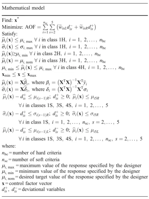
Table 4 Robust design optimization model using physical programming

Mathematical model

Find:x*

Minimize:AOF¼P

nsc

i¼1

P5 s¼2

e

wisLdisþwisRde þis

Satisfy:

b

mið Þ x mi;max8iin class 1H;i¼1;2;. . .;nhc

b

sið Þ x si;max8iin class 1H; i¼1;2;. . .;nhc

b

mið Þ≥x mi;min8iin class 2H;i¼1; 2;. . .; nhc

b

mið Þ ¼x mi;nom8iin class 3H; i¼1;2;. . .; nhc mi;minmbið Þ x mi;max8iin class 4H;i¼1;2;. . .;nhc xminxxmax

b

mið Þ ¼x Xbbi; wherebi¼ XTX

1

XTyi

b

sið Þ ¼x Xbdi; wheredi¼ XTX

1

XTsi

b

μið Þ x disþμi sð1ÞR; disþ0; bμið Þ x μi5R 8iin classes 1S;3S;4S;i¼1;2;. . .;5 b

σið Þ x d_isþσi sð1ÞR;disþ0; bσið Þ x σi5R

8iin class 1S;i¼1;2;. . .; nsc; s¼2;. . .; 5

b

μið Þ x d_isμi sð1ÞL;dis 0; bμið Þ x μi5L

8iin classes 1S;3S;4S;i¼1;2;. . .;nsc;s¼2;. . .;5 where:

nhc= number of hard criteria

nsc= number of soft criteria

mi;max= maximum value of the response specified by the designer mi;min= minimum value of the response specified by the designer mi;nom= desired target value of the response specified by the designer

(9)

attributes considered in this example are found as follows:

b

μ1ð Þ ¼x 175þ12x1þ15:3x2þ29:2x3þ4:2x211:3x22þ16:8x23þ7:7x1x2þ5:1x1x3þ14:1x2x3 b

σ1ð Þ ¼x 25:2þ2:8x1þ1:06x2þ0:55x3þ2:94x218:14x 2

22:72x 2

3þ6:71x1x2þ9:35x1x3þ2:15x2x3 b

μ2ð Þ ¼x 84:9þ5:3x1þ0:24x2þ8:80x30:52x2111:80x22þ0:39x23þ0:22x1x2þ3:60x1x34:42x2x3 b

σ2ð Þ ¼x 25:4þ0:2x1þ0:031x2þ0:4x32:741x218:91x222:54x23þ6:397x1x2þ9:243x1x3þ1:601x2x3 b

μ3ð Þ ¼x 39:7þ3:6x1þ1:002x2þ2:26x3þ2:542x219:69x 2

22:37x 2

3þ6:083x1x2þ9:135x1x3þ1:051x2x3 b

σ3ð Þ ¼x 33:3þ1:8x1þ0:0999x2þ3:0x3þ2:311x2111:60x222:17x23þ5:823x1x2þ9:398x1x3þ0:114x2x3

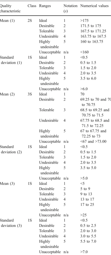
The attributes of each of the quality characteristics are then classified and the designer’s preferences are specified. This information is shown in Table5 and is based on the designer’s judgment concerning the system under investi-gation. The next step is to assess the weights based on the preferences of the designer. For demonstration purposes, only the derivation of the weights for the mean of the tensile strength ðbm₁ð Þx Þ is shown here. First, the rates of change along the horizontal axis are calculated using Eq.2:

b

μ12L¼175171:25¼3:75 b

μ13L¼171:25167:5¼3:75 b

μ14L¼167:5163:75¼3:75 b

μ15L¼163:75160¼3:75

The rates of change along the vertical axis are determined using Eq.5:

γ¼1:1 nsc¼6 ec2¼0:1

ec3¼1:1ð61Þ 0:1¼0:55 ec4¼1:1ð61Þ 0:55¼3:025 ec5¼1:1ð61Þ 3:025¼16:6375

Then, using the results from the previous calculations, the slopes are computed using Eq.7:

w12L¼ 0:1

3:75¼0:0267

w13L¼ 0:55

3:75¼0:1466

w14L¼ 3:025

3:75 ¼0:8066

w15L¼ 16:637

3:75 ¼4:4366

Finally, the weights are calculated using Eq.10:

e

w12L¼0:02670¼0:0267 e

w13L¼0:14660:0267¼0:1199 e

w14L¼0:80660:1466¼0:66 e

w15L¼4:43660:8066¼3:63

This procedure is also used to determine the weights for the attributes of the other quality characteristics of interest in this example, all of which are then combined with the deviation variables and summed to form the AOF. Based on the model given in Table4 and the AOF given in Eq. 13, the optimal process parameter settings found using PhyOpt are shown in Table6.

4.1 Discussion

(10)

class of the quality characteristic of interest. For soft classes, this would involve a re-determination of the designer’s preferences to meet the specifications for the new class. For hard classes, the constraints in the model can be easily updated once the new target value is specified. The second possible type of categorization change involves case changes, where it is necessary to re-categorize soft cases as hard cases or vice versa. Here, the model can be updated to accommodate the new model constraints or revised AOF, respectively, depending on the necessary categorization change. The most significant design change possible in the proposed process is the addition or subtraction of quality characteristics to or from the model. If it is necessary to add a new quality characteristic to the design problem, the entire approach shown in Fig.3can be completed for the additional quality characteristic. Oppo-sitely, if a quality characteristic is removed from the design problem, its constraints or weights are simply removed from the optimization model, which is then re-optimized, as discussed previously. The independent nature of the steps in the proposed process provides flexibility in terms of the design approach, such that changes to the design problem are easily incorporated into the existing model. Using this approach, new information is combined with the existing knowledge about the design to revise the model, as opposed to having to redesign the entire optimization model.

4.2 Sensitivity analysis

[image:10.595.52.286.79.613.2]

A sensitivity analysis was completed for the numerical example considered in this paper in order to study the effect of varying the input variables on the results of the proposed optimization model. In this investigation, which is shown in Table 7, the design factors (x1*, x2*, x3*) for the tablet manufacturing problem are varied in the leftmost columns of the table and the calculations of the effect on the process meanðbm_ið Þx Þand standard deviationðbsið Þx Þ;as well as the objective function (AOF) are shown on the right side of the table. The results of this study show how changes in design factors affect the outputs of the system under investigation, and the minimum value of the objective function is highlighted on the right side of the table. The results of our proposed methodology are validated by this study because the minimum value of the objective function corresponds to the optimum operating conditions found using our proposed methodology, which are highlighted on the left side of Table7.

Table 6 The optimal design factor settings for the tablet manufacturing problem

x1* x2* x3* mb1ð Þx bs1ð Þx mb2ð Þx bs2ð Þx bm3ð Þx sb3ð Þx t6.1

−0.844 1.070 1.257 252.65 0.014 68.482 0.038 13.734 5.475

t6.2

Table 5 Preferences of the designer for the tablet manufacturing problem

Quality characteristic

Class Ranges Notation (s)

Numerical values

Mean (1) 2S Ideal 1 >175

Desirable 2 171.5 to 175

Tolerable 3 167.5 to 171.25

Undesirable 4 163.75 to 167.5 Highly

undesirable

5 160 to 163.75

Unacceptable n/a <160 Standard

deviation (1)

1S Ideal 1 <0.5

Desirable 2 0.5 to 1.5

undesirable

5 3.5 to 6.0

Unacceptable n/a >6.0

Mean (2) 3S Ideal 1 70

Desirable 2 69.25 to 70 and 70 to 70.75

Tolerable 3 68.5 to 69.25 and 70.75 to 71.5 Undesirable 4 67.75 to 68.5 and

71.5 to 72.25 Highly

undesirable

5 67 to 67.75 and

72.25 to 73 Unacceptable n/a <67 and >73.00 Standard

deviation (2)

1S Ideal 1 <0.5

undesirable

5 3.5 to 5.0

Unacceptable n/a >5.0

Mean (3) 1S Ideal 1 <5

Desirable 2 5 to 9

Tolerable 3 9 to 13

Undesirable 4 13 to 17

Highly undesirable

5 17 to 25

Unacceptable n/a >25 Standard

deviation (3)

1S Ideal 1 <0.5

undesirable

5 5.5 to 7.0

[image:10.595.177.546.675.718.2]

(11)

[image:11.595.53.548.55.445.2]

Table 7 Sensitivity analysis for the tablet manufacturing problem

x1* x2* x3* bm1ð Þx sb1ð Þx bm2ð Þx sb2ð Þx bm3ð Þx bs3ð Þx AOF

−0.840 1.043 1.306 256.10 0.016 69.465 0.105 13.933 5.832 8.7895

−0.676 1.138 1.349 265.60 0.685 68.385 0.005 14.32 5.414 8.0722

−0.909 1.037 1.223 247.90 0.019 68.731 0.325 13.787 5.809 9.1810

−0.821 1.067 1.285 255.30 0.149 68.896 0.112 13.93 5.667 7.4873

−0.648 1.131 1.377 268.46 1.074 69.011 0.333 14.798 5.898 10.600

−0.668 1.128 1.363 266.73 0.888 68.840 0.214 14.595 5.740 8.9154

−0.844 1.070 1.257 252.62 0.014 68.482 0.038 13.734 5.475 6.2544

−0.804 1.073 1.301 257.15 0.129 68.938 0.027 13.930 5.602 6.7051

−0.658 1.141 1.363 267.33 0.833 68.528 0.088 14.484 5.53 6.9503

−0.829 1.081 1.251 252.73 0.117 68.294 0.066 13.789 5.443 9.0307

−0.602 1.161 1.401 272.52 1.167 68.582 0.184 14.796 5.634 8.2775

−0.785 1.084 1.303 257.99 0.232 68.810 0.041 13.997 5.577 6.6495

−0.806 1.075 1.280 255.41 0.303 68.806 0.203 14.060 5.721 8.3045

[image:11.595.51.550.546.717.2]

(12)

5 Conclusion

In this paper, we proposed an extension to the multi-response robust design (RD) problem considering the use of physical programming. We described our proposed meth-odology in detail, demonstrated it through the use of a numerical example, and validated our findings with a sensitivity study. The model proposed here is unique because it incorporates a methodology for clearly defining priorities in multiresponse problems. Here, physical programming was used in the context of RD as a precise tool for capturing designer’s preferences with a reasonable degree of accuracy and transforming these into specific weighted objectives. This approach, along with incorporat-ing goal programmincorporat-ing techniques into the traditional multiresponse RD problem, ensures the flexibility neces-sary in the development phase.

Our proposed model considers both multiple, conflicting objectives and design flexibility, in that changes to the design problem, which inevitably occur during the design process, are easily accommodated by our approach. By extending the current knowledge of physical programming and linking the concept of experimental design to RD, this paper develops the logistics of experiment-based RD with the consideration of multiple quality characteristics. As knowledge about the design evolves throughout the design timeline, the optimization model is easily adjusted in order to determine new optimum operating conditions. It is the independence of the model components in this approach that allows the model to be updated easily when given new information. The model is updated in such a way that revised information can be combined with prior information about the problem so that the model can be easily re-solved with minimal effort. Therefore, the proposed methodology supports human judgment involved in the decision-making process encountered in all design problems and allows products and processes to be designed more efficiently to meet customers’ needs. The source code concerning the optimization software used in this paper, PhyOpt, can be forwarded upon a request made to the authors.

References

1. Taguchi GW (1986) Introduction to quality engineering. Krauss International Publications, White Plains, New York

2. Taguchi GW (1987) Systems of experimental design: engineering methods to optimize quality and minimize cost. Quality Resour-ces, White Plains, New York

3. Taguchi GW, Wu YI (1985) Introduction to off-line quality control. American Supplier Institute, Dearborn, Michigan

4. Phadke MS (1989) Quality engineering using robust design. Prentice Hall, Englewood Cliffs, New Jersey

5. Kackar RN (1985) Off-line quality control, parameter design, and the Taguchi method. J Qual Tech 17(4):176–188

6. Kackar RN (1986) Taguchi’s quality philosophy: analysis and commentary. Qual Prog 19(12):21–29

7. Leon RV, Shoemaker AC, Kackar RN (1987) Performance measures independent of adjustment: an explanation and extension of Taguchi’s signal-to-noise ratios. Technometrics 29(3):253–285 8. Box GEP (1988) Signal-to-noise ratios, performance criteria, and

transformations. Technometrics 30(1):1–17

9. Box GEP, Bisgaard S, Fung C (1988) An explanation and critique of Taguchi’s contributions to quality engineering. Int J Relia Mgt 4(2):123–131

10. Pignatiello JJ Jr, Ramberg JS (1991) Top ten triumphs and tragedies of Genichi Taguchi. Qual Eng 4(2):211–225

11. Nair VN (1992) Taguchi’s parameter design: a panel discussion. Technometrics 34(2):127–161

12. Tsui KL (1992) An overview of Taguchi method and newly developed statistical methods for robust design. IIE Trans 24 (5):44–57

13. Myers RH (1999) Response surface methodology—current status and future directions. J Qual Tech 31(1):30–44

14. Vining GC, Myers RH (1990) Combining Taguchi and response surface philosophies: a dual response approach. J Qual Tech 22 (1):38–45

15. del Castillo E, Montgomery DC (1993) A nonlinear programming solution to the dual response problem. J Qual Tech 25(3):199–204 16. Copeland KAF, Nelson PR (1996) Dual response optimization via

direct function minimization. J Qual Tech 28(3):331–336 17. Cho BR (1994) Optimization issues in quality engineering. PhD

thesis, University of Oklahoma, Oklahoma

18. Lin DKJ, Tu W (1995) Dual response surface optimization. J Qual Tech 27(1):34–39

19. Kim YJ, Cho BR (2000) Economic consideration on parameter design. Qual Reliab Eng Int 16:501–514

20. Parkinson DB (2000) Robust design employing a genetic algorithm. Qual Reliab Eng Int 16(3):201–208

21. Brenneman WA, Myers WR (2003) Robust parameter design with categorical noise variables. J Qual Tech 35(4):335–341

22. Köksoy O, Doganaksoy N (2003) Joint optimization of mean and standard deviation using response surface methods. J Qual Tech 35(3):239–252

23. Miro-Quesada G, del Castillo E (2004) Two approaches for improving the dual response method in robust parameter design. J Qual Tech 36(2):154–168

24. Shin SM, Cho BR (2005) Bias-specified robust design optimiza-tion and its analytical soluoptimiza-tions. Comp Ind Eng 48(1):129–140 25. Harrington EC (1965) The desirability function. Ind Qual Cont 21

(10):494–498

26. Derringer G, Suich R (1980) Simultaneous optimization of several response variables. J Qual Tech 12(4):214–219

27. Khuri AI, Conlon M (1981) Simultaneous optimization of multiple responses represented by polynomial regression func-tions. Technometrics 23(4):363–375

28. Pignatiello JJ (1993) Strategies for robust multi-response quality engineering. IIE Trans 25(3):5–15

29. Messac A (1996) Physical programming: effective optimization for computational design. AIAA J 34(1):149–158

30. Messac A (2000) From the dubious construction of objective functions to the application of physical programming. AIAA J 38 (1):155–163

(13)

32. Chen W, Sahai A, Messac A, Sundararaj GJ (2000) Exploration of the effectiveness of physical programming in robust design. J Mech Des 122(2):155–163

33. Messac A, Ismail-Yahaya A (2001) Multiobjective robust design using physical programming. Struc Multidiscip Opt 23(5):357– 371

34. Logothetis N, Haigh A (1988) Characterizing and optimizing multi-response processes by Taguchi method. Qual Relia Eng Int 4(2):159–169

35. Elsayed EA, Chen A (1993) Optimal levels of process parameters for products with multiple characteristics. Int J Prod Res 31 (5):1117–1132

36. Ames AE, Mattucci N, MacDonald S, Szonyi G, Hawkins DM (1997) Quality loss functions for optimization across multiple response surfaces. J Qual Tech 29(3):339–346

37. Derringer GC (1994) A balancing act: optimizing a product’s properties. Qual Prog 27(6):51–58

38. Kapur KC, Cho BR (1996) Economic design of the specification region for multiple quality characteristics. IIE Trans 28(3):237–248 39. Su C-T, Tong L-I (1997) Multi-response robust design by

principal component analysis. Total Qual Mgt 8(6):409–416 40. Tong L-I, Su C-T (1997) Optimizing multi-response problems in

the Taguchi method by fuzzy multiple attribute decision making. Qual Relia Eng Int 13(1):25–34

41. Tong L-I, Su C-T, Wang C-H (1997) The optimization of multi-response problems in the Taguchi method. Int J Qual and Relia Mgt 14(4):367–380

42. Chen L-H (1997) Designing robust products with multiple quality characteristics. Comp Oper Res 24(10):937–944

43. Kim K, Lin DKJ (1998) Dual response surface optimization: a fuzzy modeling approach. J Qual Tech 30(1):1–10

44. Vining GG (1998) A compromise approach to multiresponse optimization. J Qual Tech 30(3):309–313

45. Tsui KL (1999) Robust design optimization for multiple charac-teristic problems. Int J Prod Res 37(2):433–445

46. Chiao C-H, Hamada M (2001) Analyzing experiments with correlated multiple responses. J Qual Tech 33(4):451–465 47. Kim YJ, Cho BR (2002) Development of priority-based robust

design. Qual Eng 14(3):355–363

48. Tang LC, Xu K (2002) A unified approach for dual response surface optimization. J Qual Tech 34(4):437–447

49. Lin CL, Lin JL, Ko TC (2002) Optimization of the EDM process based on the orthogonal array with fuzzy logic and grey relational analysis method. Int J Adv Manuf Tech 19(4):271–277

50. Lu D, Antony J (2002) Optimization of multiple responses using a fuzzy-rule based inference system. Int J Prod Res 40(7):1613–1625 51. Romano D, Varetto M, Vicario G (2004) Multiresponse robust design: a general framework based on combined array. J Qual Tech 36(1):27–37

52. Wu F-C, Chyu C-C (2004) Optimization of robust design for multiple quality characteristics. Int J Prod Res 42(2):337–354 53. Hillier FS, Lieberman GJ (2001) Introduction to operations

research. McGraw-Hill, New York