WITH NONLINEAR CROSSWIND DIFFUSION FOR CONVECTION-DIFFUSION-REACTION EQUATIONS
GABRIEL R. BARRENECHEA, VOLKER JOHN, AND PETR KNOBLOCH
Abstract. An extension of the local projection stabilization (LPS) finite element method for convection-diffusion-reaction equations is presented and analyzed, both in the steady-state and the transient setting. In addition to the standard LPS method, a nonlinear cross-wind diffusion term is introduced that accounts for the reduction of spurious oscillations. The existence of a solution can be proved and, depending on the choice of the stabiliza-tion parameter, also its uniqueness. Error estimates are derived which are supported by numerical studies. These studies demonstrate also the reduction of the spurious oscillations.
1. Introduction
The solution of convection-dominated convection-diffusion-reaction equations with finite element methods constitutes a very challenging (and open) problem. Over the last three decades, the amount of work devoted to this problem is impressive. The usual way of treating dominating convection, at least in the context of finite element methods, consists in adding extra terms to the standard Galerkin formulation, aimed at enhancing the stability of the discrete solution by means of introducing artificial diffusion. These new terms vary according to the method, and can be residual-based, as in the SUPG/GLS/SDFEM family (see [6, 16, 13, 14, 29]), or edge based, such as the CIP method (see [9, 7]). For an up-to-date and thorough review of these and other techniques, see [31]. It is striking to notice that, despite the impressive amount of work that has been devoted to this topic, up to now there is not a method that ’ticks all the boxes’, i.e., a method that produces sharp layers while avoiding oscillations, see [1] for a recent review and a numerical assessment.
Among the various stabilized finite element methods, the local projection stabilization (LPS) method has received some attention over the last decade. Originally proposed for the Stokes problem in [2], and extended to the Oseen equations in [4] (see also [5, 30]), the LPS method has been also used recently to treat convection-diffusion equations (see
Date: March 5, 2013.
Key words and phrases. finite element method; local projection stabilization; crosswind diffusion; convection-diffusion-reaction equation; well posedness; time dependent problem; stability; error estimates.
1
[26, 15, 24, 25]). The basic idea of this method consists in restricting the direct application of the stabilization to so-called fluctuations or resolved small scales, which are defined by local projections. It has several attractive features, such as adding symmetric terms to the formulation and avoiding the computation of second derivatives of the basis functions (thus using only information that is needed for the assembly of the matrices from the standard Galerkin method). Unfortunately, the solutions obtained with the LPS method possess the same deficiency like solutions computed, e.g., with the SUPG method: non-negligible spurious oscillations are often present in a vicinity of layers.
Motivated by the wish of recovering the monotonicity properties of the continuous prob-lem, which might be crucial in applications, a number of so-called Spurious Oscillations at Layers Diminishing (SOLD) methods were proposed. SOLD methods add an extra term to the already stabilized formulation, which usually depends on the discrete solution in a nonlinear way, vanishes for small residuals (thus acting mostly at layers), and adds some extra, but different, diffusivity to the formulation. In particular, methods that add cross-wind diffusion, like the one proposed in [11], have been proved to belong to the best SOLD methods in comprehensive studies [17, 18]. Although these methods diminish oscillations considerably, no single method succeeds to fully eliminate them [17, 18, 23]. Also, from a purely mathematical point of view, it is unknown if these methods lead to well-posed prob-lems. In fact, existence of solutions is usually possible to prove, but, to our best knowledge, there is no nonlinear SOLD method that is known to produce a unique solution, see [27] and [7] for a discussion of this topic.
Based on the previous considerations, this paper has three major objectives, namely:
• to improve the quality of the LPS solution (especially in the vicinity of layers); • to explore the applicability of SOLD-type strategies within a LPS context; and • to contribute to the mathematical understanding of nonlinear stabilization techniques
for the convection-diffusion equation.
θ-scheme. To our best knowledge, this is the first nonlinear discretization for convection-diffusion-reaction equations for which both, existence and uniqueness of a solution can be shown. The form of the crosswind term resembles the Smagorinsky Large Eddy Simulation (LES) model which was analyzed in [28]. It involves fluctuations of a term mimicking a p -Laplacian. The crucial analytical property for proving the uniqueness of the solution is the strong monotonicity of the corresponding operator. For the more complicated local definition of the parameter, the analysis will show the existence of a solution and its uniqueness for the time-dependent discretization in the case of sufficiently small time steps.
The analysis is performed for the model problems of linear steady-state and time-dependent convection-diffusion-reaction equations. Applying a nonlinear discretization scheme to a lin-ear problem leads certainly to a considerable complication of the solution process and to an additional numerical cost. This latter aspect can be overcome in the transient regime by using a semi-implicit (linearized) approach that computes the stabilization parameter with the solution from the previous discrete time. With respect to the former aspect, it has to be mentioned that the most important motivation for studying discretizations that reduce spurious oscillations comes from the need to address applications that lead to nonlinear cou-pled systems of convection-diffusion-reaction equations as in [21]. It was demonstrated in [21] that the locally large spurious oscillations of the SUPG method might lead to a fast blow-up of the simulations, and hence the reduction of the spurious oscillations is essential to perform simulations at all. Thus, the reduction of the oscillations at layers becomes a priority, even over computational cost. It should be noted that in many applications, like in [21], only interior or characteristic layers are present, such that a method for reducing the oscillations has to work properly in particular for these types of layers. Finally, it is worth mentioning that our final aim is to address applications that lead to such coupled problems. Since these problems are nonlinear, the use of a nonlinear stabilization usually does not result in a notable complication of the solution procedure.
fit into this framework. Finally, numerical illustrations that support the analytical results and which demonstrate the reduction of spurious oscillations are presented in Section 6.
Throughout the paper, standard notations are used for Sobolev spaces and corresponding norms, see, e.g., [10]. In particular, given a measurable set D ⊂ Rd, the inner product in L2(D) or L2(D)d is denoted by (·,·)
D and the notation (·,·) is used instead of (·,·)Ω. The
norm (seminorm) in Wm,p(D) will be denoted by k · k
m,p,D (| · |m,p,D), with the convention
k · km,D =k · km,2,D, and the same notation is used for scalar and vector-valued functions.
1.1. The problems of interest. Let Ω⊂Rd,d∈ {2,3}, be a bounded polygonal
(polyhe-dral) domain with a Lipschitz-continuous boundary ∂Ω and let us consider the steady-state convection-diffusion-reaction equation
(1) −ε∆u+b· ∇u+c u=f in Ω, u=ub on∂Ω.
It is assumed that ε is a positive constant and b ∈W1,∞(Ω)d, c∈ L∞(Ω), f ∈ L2(Ω), and
ub ∈H1/2(∂Ω) are given functions satisfying
(2) σ :=c− 1
2∇ ·b ≥σ0 >0 in Ω,
where σ0 is a constant. Then the boundary value problem (1) has a unique solution in
H1(Ω).
The condition σ0 >0 is often used in the analysis of stabilized finite element methods for the numerical solution of (1), see, e.g., [31], but it limits the applications of the theory since many problems of interest involve solenoidal convective velocities and no zero-order terms, which leads to σ0 = 0. Unfortunately, it is not known how to prove optimal convergence results even for the underlying linear local projection stabilization without assuming σ0 >0, although numerical results do not indicate any deterioration of the convergence rates when
σ0 = 0. The analysis of the nonlinear term introduced in this paper does not require this assumption.
Besides the steady-state case, also the time-dependent convection-diffusion-reaction equa-tion
(3)
ut−ε∆u+b· ∇u+c u = f in (0, T]×Ω,
u = ub in [0, T]×∂Ω, u(0,·) = u0 in Ω,
will be considered. In (3), [0, T] is a finite time interval,εis assumed to be a positive constant,
b∈L∞
(0, T;W1,∞
(Ω)d),c∈L∞
(0, T;L∞
(Ω)),f ∈L2(0, T;L2(Ω)),u
b ∈L2(0, T;H1/2(∂Ω)),
and the inequality (2) is assumed to hold for allt ∈[0, T]. In this case, the condition σ0 >0 can be circumvented by considering instead of (3) an equivalent problem for v = u e−α t
which satisfies σ0 >0 for sufficiently large α.
2. Assumptions on approximation spaces and the set Mh
From now on, C, ˜C or ¯C denote generic constants which may take different values at different occurrences but are always independent of the data ε,b,c,f, andub, the constant
σ0, and the discretization parameters (h and δt in the following).
Given h > 0, let Wh ⊂ W1,∞(Ω) be a finite-dimensional space approximating the space H1(Ω) and set Vh = Wh∩H1
0(Ω). Next, let Mh be a set consisting of a finite number of
open subsets M of Ω such that Ω =∪M∈MhM. It will be supposed that, for any M ∈Mh,
card{M′
∈Mh; M ∩M′
6
=∅} ≤C ,
(4)
hM := diam(M)≤C h ,
(5)
hM ≤C hM′ ∀ M
′
∈Mh, M ∩M′
6
=∅,
(6)
hdM ≤Cmeasd(M).
(7)
The space Wh is assumed to satisfy the local inverse inequality
(8) |vh|1,M ≤C h
−1
M kvhk0,M ∀vh ∈Wh, M ∈Mh.
For any M ∈Mh, a finite-dimensional space DM ⊂ L∞
(M) is introduced. It is assumed that there exists a positive constant βLP independent ofh such that
(9) sup
v∈VM
(v, q)M
kvk0,M ≥βLPkqk0,M ∀ q ∈DM, M ∈Mh,
where VM = {vh ∈ Vh; vh = 0 in Ω\M}. This hypothesis will be needed in what follows
for the construction of a special interpolation operator (see Lemma 6 below). Concrete examples of spacesWh and DM satisfying the assumptions formulated here will be presented in Section 5.
Furthermore, for any M ∈Mh, a finite-dimensional space GM ⊂L∞
(M) withGM ⊃DM
is introduced such that
∂vh ∂xi
M
∈GM ∀ vh ∈Wh, i= 1, . . . , d ,
and it is assumed that, for any p∈[1,∞], there is a constant C such that
(10) kqk0,p,M ≤C h
d p−
d 2
To characterize the approximation properties of the spaces Wh and DM, it is assumed that there exist interpolation operators ih ∈ L(C(Ω), Wh) ∩L(C(Ω) ∩ H1
0(Ω), Vh) and
jM ∈ L(H1(M), DM), M ∈ M
h, such that, for some constants l ∈ N and C > 0 and for
any set M ∈Mh, it holds
|v−ihv|1,M +h−1
M kv−ihvk0,M ≤C hkM|v|k+1,M ∀ v ∈Hk+1(M), k= 1, . . . , l ,
(11)
kq−jMqk0,M ≤C hkM|q|k,M ∀ q∈Hk(M), k = 1, . . . , l .
(12)
In addition, it is assumed that, for any p∈[1,6],
(13) |v−ihv|1,p,M ≤C hk+
d p−
d 2
M |v|k+1,M ∀ v ∈Hk+1(M), k = 1, . . . , l .
3. A local projection discretization of the steady-state problem
The weak form of problem (1) is: Find u∈H1(Ω) such that u=ub on∂Ω and
a(u, v) = (f, v) ∀ v ∈H01(Ω),
(14)
where the bilinear form a is given by
a(u, v) :=ε(∇u,∇v) + (b· ∇u, v) + (c u, v).
As it was mentioned in the introduction, the most often used approach to cure the insta-bilities of the Galerkin method consists in adding extra terms to the formulation. To build these additional terms for the method studied here, for any M ∈ Mh, a continuous linear projection operator πM is introduced which maps the space L2(M) onto the space DM. It is assumed that
(15) kπMkL(L2(M),L2(M))≤C ∀ M ∈Mh.
E.g., if πM is the orthogonal L2 projection, thenC = 1. Using this operator, the fluctuation operatorκM :=id−πM is defined, whereidis the identity operator onL2(M). Then, clearly
(16) kκMkL(L2(M),L2(M))≤C ∀ M ∈Mh.
Since κM vanishes onDM, it follows from (16) and (12) that
(17) kκMqk0,M ≤C hkM|q|k,M ∀ q∈Hk(M), M ∈Mh, k = 0, . . . , l .
An application of κM to a vector-valued function means thatκM is applied component-wise.
For any M ∈Mh, a constant bM ∈Rd is chosen such that
(18) |bM| ≤ kbk
where | · | denotes the Euclidean norm in Rd. A typical choice for bM is the value of b at
one point ofM, or the integral mean value of b over M. In addition, a function eubh∈Wh is
introduced such that its trace approximates the boundary conditionub.
We are now ready to present the finite element method to be studied: Finduh ∈Wh such that uh−eubh ∈Vh and
a(uh, vh) +sh(uh, vh) +dh(uh;uh, vh) = (f, vh) ∀ vh ∈Vh,
(19)
where
sh(u, v) = X
M∈Mh
τM (κM(bM · ∇u), κM(bM · ∇v))
M ,
dh(w;u, v) = X
M∈Mh
τMsold(w)κM(PM∇u), κM(PM∇v)M ,
and PM : Rd → Rd is the projection onto the line (plane) orthogonal (crosswind) to the
vector bM defined by
PM =
I− bM ⊗bM
|bM|2 if bM 6=0,
0 if bM =0,
I being the identity tensor. The stabilization parameters are given by
τM =τ0 min
(
hM
kbk
0,∞,M ,h
2
M ε
)
,
(20)
τMsold(uh) = ˜τM(uh)|κM(PM∇uh)|,
where τ0 is a positive constant and ˜τM is a non-negative function ofuh and the data of (1). Note that the crosswind stabilization term is of p-Laplacian type with p= 3.
It remains to specify the function ˜τM. First, inspired by the definition of sh, where each term in the sum is bounded by τ0hM|bM| kκM∇uk0,MkκM∇vk0,M, we set ˜τM(uh) = γM(uh)hM|bM|with a functionγM still depending onuh and/or the data of (1). Second, the
functionγM has to be chosen in such a way that the discrete problem preserves the following scaling properties of the problem (1):
• if the data ε, b, c, and f are replaced by α ε, αb, α c, and α f, respectively, with
some constantα 6= 0, then the solution of (1) does not change;
• if f and ub are replaced by α f and α ub, respectively, then u changes to α u;
• if Ω is transformed to F−1(Ω) with F(x) = x/α, then u◦F solves an analog of (1) inF−1
Note that the discrete problem (19) without the nonlinear termdh preserves these properties. To preserve the properties also when using the nonlinear term, the functionγM has to satisfy
γM(ε,b, c, f, ub,Ω, uh) =γM(α ε, αb, α c, α f, ub,Ω, uh)
=α γM(ε,b, c, α f, α ub,Ω, α uh)
=α−1γ
F−1(M)(α2ε, αb◦F, c◦F, f ◦F, ub◦F, F−1(Ω), uh◦F)
for any admissible data, α 6= 0, and uh ∈Wh. We shall consider two choices of the scaling functionγM: a global one independent of uh and a local one depending on uh. In the former case, one may set
(21) γM =γ0diam(Ω)d/2 k
fk0,Ωdiam(Ω)
ε+kbk
0,∞,Ωdiam(Ω) +kck0,∞,Ωdiam(Ω)2
+ kubk0,∂Ω diam(Ω)1/2
!−1
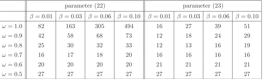
with a positive constant γ0. The local scaling can be defined by settingγM =β hd/M2/|uh|1,M
with a positive constant β if |uh|1,M 6= 0. Thus, we arrive at the following two formulas for
the function ˜τM:
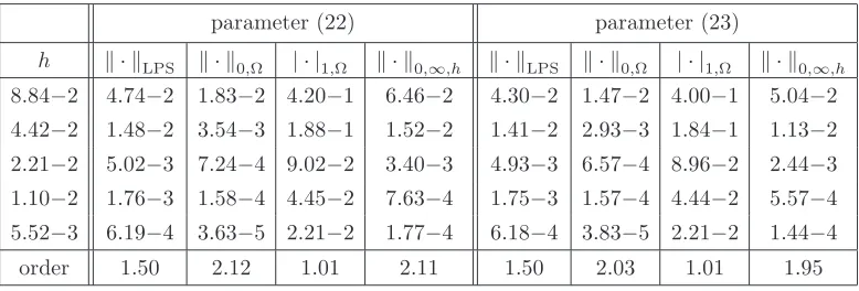
(22) τM˜ =β hM |bM|,
and
(23) τM˜ (uh) =
β h1+Md/2|bM|
|uh|1,M if |uh|1,M 6= 0,
0 if |uh|1,M = 0,
where β is a positive real number independent of uh and h. The parameter β depends on the data of (1) in case of (22) (e.g., like γM in (21)), but it is independent of the data of (1) in case of (23). For these two choices of ˜τM, we shall investigate the properties of the
discrete problem (19). Although the local scaling is likely to lead to better numerical results than the global one, we consider both variants since the choice (22) turns out to be more appealing for the analysis.
Remark.
• If d = 2 and bM 6= 0, one has PM = b⊥
M ⊗ b ⊥
M where b ⊥
M is a vector satisfying
b⊥
M ·bM = 0 and |b ⊥
M| = 1. Thus, in this case, the nonlinear stabilization term can
be written in the form
dh(w;u, v) =
X
M∈Mh
(τMsold(w)κM(b ⊥
M · ∇u), κM(b ⊥
• It is useful for the analysis of the discrete problem to note that κM(bM · ∇u) = bM ·κM∇u and κM(PM∇u) =PMκM∇u. Note also that kPMk
2 = 1.
• Finally, if ˜τM is defined by (23), then, using the stability of κM and bM (18) and
(16), respectively, and kPMk2 = 1, one obtains
(24) kτMsold(v)k0,M ≤C h1+Md/2kbk
0,∞,M ∀ v ∈H1(Ω), M ∈Mh.
In the analysis, the error will be measured using the following mesh-dependent norm
kvkLPS:= ε|v|21,Ω+kσ1/2vk20,Ω+sh(v, v)1/2 ,
and a term involving the crosswind derivative of the error. Note that integrating by parts gives
(25) a(v, v) +sh(v, v) = kvk2
LPS ∀ v ∈H01(Ω).
3.1. Well-posedness of the nonlinear discrete problem. This section studies the ex-istence and uniqueness of solutions for the nonlinear discrete problem (19). The results of this section are valid also for σ0 = 0.
Let us define the nonlinear operator Th :Vh →Vh by
(Thzh, vh) =a(zh +ubh, vhe ) +sh(zh+eubh, vh) +dh(zh+eubh;zh+eubh, vh)−(f, vh) (26)
for any zh, vh ∈Vh. Then uh∈Wh is a solution of (19) if and only ifuh|∂Ω =eubh|∂Ω and
Th(uh−uebh) = 0,
or, equivalently, uh =ueh +uebh∈ Wh is a solution of (19) if euh ∈ Vh and Th(ueh) = 0.Thus,
our aim is to prove that the operator Th has a zero in Vh. To this end, the properties of the form dh shall be investigated first. As these properties are different with respect to the definition of ˜τM, we start supposing that ˜τM is given by (22).
Lemma 1. Let τM˜ be defined by (22). Consider any u, v, z ∈W1,3(Ω) and set w :=u−v. Then
dh(u;u, w)−dh(v;v, w)≥ 1 7
X
M∈Mh ˜
τMkκM(PM∇w)k30,3,M = 1
7dh(w;w, w), (27)
|dh(u;u, z)−dh(v;v, z)| ≤ X
M∈Mh ˜
τM(kκM(PM∇u)k0,3,M +kκM(PM∇v)k0,3,M)
(28)
Proof. Let us denote
(29) dh(u;u, z)−dh(v;v, z) =
X
M∈Mh
NM(u, v, z),
where
NM(u, v, z) := τMsold(u)κM(PM∇u)−τMsold(v)κM(PM∇v), κM(PM∇z)M .
For t∈[0,1], let ut:=tu+ (1−t)v and set
g(t) := ˜τM|κM(PM∇ut)|κM(PM∇ut), t∈[0,1].
Then
NM(u, v, z) = g(1)−g(0), κM(PM∇z)
M =
Z 1
0
g′
(t) dt, κM(PM∇z)
M .
Since
(30) g′(t) = ˜τM κM(PM∇u t)
|κM(PM∇ut)|κM(PM∇u
t)·κM(PM∇w) + ˜τM|κM(PM∇ut)|κM(PM∇w),
one has
|g′(t)| ≤2 ˜τM |κM(PM∇ut)| |κM(PM∇w)|
≤2 ˜τM (t|κM(PM∇u)|+ (1−t)|κM(PM∇v)|)|κM(PM∇w)|,
which implies (28). On the other hand, since multiplication of the first term on the right-hand side of (30) by κM(PM∇w) gives a non-negative expression, one obtains
(31) NM(u, v, w)≥
˜
τM
Z 1
0 |
κM(PM∇ut)|dt κM(PM∇w), κM(PM∇w)
M .
Next, clearly
Z 1
0 |
κM(PM∇ut)|dt≥ max
i=1,...,d
Z 1
0 |
t κM(PM∇u)i+ (1−t)κM(PM∇v)i|dt .
Denoting
I(a, b) =
Z 1
0 |
ta+ (1−t)b|dt , a, b∈R,
a direct computation gives
I(a, b) = |a|+|b|
2 if a b≥0, I(a, b) = 1 2
a2+b2
|a|+|b| if a b < 0.
Thus, for any a, b∈R, it follows
I(a, b)≥ |a|+|b|
4 ≥
|a−b|
Consequently,
Z 1
0 |
κM(PM∇ut)|dt≥ 1
4 i=1max,...,d|κM(PM∇w)i| ≥
1
4√d|κM(PM∇w)| ≥
1
7|κM(PM∇w)|.
Combining this estimate with (31) and using (29) gives (27).
Next, the properties of dh are explored for the case that ˜τM is defined by (23).
Lemma 2. Let τ˜M be defined by (23). Consider any u, v, z∈W1,4(Ω). Then
|dh(u;v, z)| ≤C X
M∈Mh
h1+Md/2kbk
0,∞,MkκM(PM∇v)k0,4,MkκM(PM∇z)k0,4,M,
(32)
|dh(u;u, z)−dh(v;v, z)| ≤C
X
M∈Mh
h1+Md/2kbk
0,∞,MζM(u, v)×
(33)
×(kκM(PM∇u)k0,4,M +kκM(PM∇v)k0,4,M)kκM(PM∇z)k0,4,M,
where
ζM(u, v) =
|u−v|1,M
|u|1,M +|v|1,M if |u|1,M 6= 0 or |v|1,M 6= 0,
0 if |u|1,M =|v|1,M = 0.
Proof. Denoting
dM(u;v, z) = τMsold(u)κM(PM∇v), κM(PM∇z)
M ,
it is easy to realize that
dh(u;v, z) = X
M∈Mh
dM(u;v, z).
Applying H¨older’s inequality yields
|dM(u;v, z)| ≤ kτMsold(u)k0,MkκM(PM∇v)k0,4,MkκM(PM∇z)k0,4,M,
which, using (24), gives
(34) |dM(u;v, z)| ≤C h1+Md/2kbk
0,∞,MkκM(PM∇v)k0,4,MkκM(PM∇z)k0,4,M,
thus proving (32). Now it will be shown that
|dM(u;u, z)−dM(v;v, z)| ≤C h1+Md/2kbk
0,∞,MζM(u, v)
(35)
If|u|1,M = 0 or |v|1,M = 0, then (35) is a particular case of (34). Thus, it suffices to consider
the case |u|1,M 6= 0, |v|1,M 6= 0. Denoting ξ(x) = |x|x, one obtains
dM(u;u, z)−dM(v;v, z) = β h 1+d/2
M |bM|
|u|1,M ξ(κM(PM∇u))−ξ(κM(PM∇v)), κM(PM∇z)
M
+β h1+Md/2|bM| 1 |u|1,M −
1 |v|1,M
!
ξ(κM(PM∇v)), κM(PM∇z)M.
(36)
The integral terms on M possess the same structure as the term NM(u, v, z) in the proof of Lemma 1 (the second term corresponds toNM(0, v, z)). They are estimated using the same technique, only with a different H¨older inequality. Then, (16) is applied to kκM(PM∇(u−v))k0,M resp.kκM(PM∇v)k0,M. Furthermore, the first inequality from (18) is
employed. To finish the estimate of the second term in (36), the triangle inequality is used. One obtains
|dM(u;u, z)−dM(v;v, z)| ≤C h1+Md/2kbk
0,∞,M
|u−v|1,M
|u|1,M
×(kκM(PM∇u)k0,4,M+kκM(PM∇v)k0,4,M)kκM(PM∇z)k0,4,M.
The same type of inequality follows by interchanging u and v. Then, using the sharper of these two estimates and min{|u|−1
1,M,|v| −1
1,M} ≤2/(|u|1,M+|v|1,M) gives (35).
The properties of the operatorTh, namely its monotonicity and local Lipschitz continuity, follow now by the results of the two previous lemmas and the representation of the LPS norm (25).
Lemma 3. If τM˜ is defined by (22), then the operator Th defined in (26) is locally Lipschitz-continuous and strongly monotone, i.e., it satisfies
(37) (Thwh−Thzh, wh−zh)≥ kwh−zhk2LPS+ 1 7
X
M∈Mh ˜
τMkκM(PM∇(wh−zh))k30,3,M
for all wh, zh ∈ Vh. If τM˜ is defined by (23), then the operator Th is Lipschitz-continuous and it satisfies
(38) (Thzh, zh)≥ ε 2|zh|
2
1,Ω−C0(kubhe k12,Ω+kfk20,Ω)
for all zh ∈Vh, where C0 >0 depends on ε, b, and c, but not on zh, h, and σ0
Proof. Let us define the operatorsAh, Nh :Vh →Vh by
(Ahzh, vh) =a(zh, vh) +sh(zh, vh) ∀ zh, vh ∈Vh,
Then, for any wh, zh ∈Vh, there holds
Thwh−Thzh =Ah(wh−zh) +Nhwh −Nhzh.
The operatorAh is linear on a finite-dimensional space and hence it is Lipschitz continuous. Thus, the (local) Lipschitz-continuity of Th follows from (28), (33), and the equivalence of norms on finite-dimensional spaces. The strong monotonicity (37) follows from (25) and (27). Finally, let ˜τM be defined by (23). In view of (25), it holds
(Thzh, zh) = kzhk2
LPS+dh(zh+eubh;zh, zh) (39)
+a(eubh, zh) +sh(ubh, zhe ) +dh(zh+eubh;ubh, zhe )−(f, zh).
Applying (32), (10), (16), (18), (4), and (5), one obtains
|dh(zh+eubh;ubh, zhe )| ≤C hkbk
0,∞,Ω|eubh|1,Ω|zh|1,Ω.
The same estimate also holds forsh(ubh, zhe ). Using the fact thatdh(zh+ubhe ;zh, zh)≥0 and applying the Cauchy–Schwarz inequality to the third and last term on the right-hand side of (39), one derives
(Thzh, zh)≥ε|zh|21,Ω−(ε+Ckbk
0,∞,Ω+kck0,∞,Ω)kubhe k1,Ωkzhk1,Ω− kfk0,Ωkzhk0,Ω.
Now, employing the Poincar´e and Young inequalities, one obtains (38).
To prove that the discrete problem (19) has at least one solution, we shall use the following simple consequence of Brouwer’s fixed-point theorem, whose proof can be found in [32, p. 164, Lemma 1.4].
Lemma 4. Let X be a finite-dimensional Hilbert space with inner product (·,·) and norm k·k. LetP :X→X be a continuous mapping andK >0a real number such that(P x, x)>0 for any x∈X with kxk=K. Then there exists x∈X such thatkxk ≤K and P x= 0.
Collecting the previous results, the main result of this section can be stated now, namely, the well-posedness of the problem (19).
Theorem 5. If τM˜ is defined by (22) or (23), then the problem (19) has a solution. If τM˜ is defined by (22), the solution of (19) is unique.
Proof. If ˜τM is defined by (22), then it follows from the strong monotonicity (37) that, for any zh ∈Vh,
(Thzh, zh)≥ kzhk2
Thus, using Young’s inequality and the equivalence of norms in the space Vh one gets
(Thzh, zh)≥C1kzhk20,Ω−C2,
whereC1,C2 are positive constants that depend on hand the data of (1), but not onzh and
σ0. According to (38), the same inequality holds if ˜τM is defined by (23). Thus, in view of Lemma 4 with any K > pC2/C1, the operator Th has a zero and hence the problem (19)
has a solution. The uniqueness in the case that ˜τM is defined by (22) follows from the strong
monotonicity (37).
3.2. Error estimates. For the analysis of the methods introduced in Section 3, we will need an appropriate interpolation operator. An important tool for the construction of such an operator is provided by the following result, whose proof can be found in [25, Lemma 1].
Lemma 6. Let us suppose the inf-sup condition (9) to be satisfied. Then, there exists an operator ̺h :L2(Ω)→Vh such that, for any v, w∈L2(Ω), the estimates
|(v−̺hv, w)| ≤C X M∈Mh
kvk0,MkκMwk0,M,
(40)
|̺hv|2 1,M+h
−2
M k̺hvk20,M ≤C
X
M′∈M h,
M∩M′6=∅
h−M2′kvk
2
0,M′ ∀ M ∈Mh
(41)
are valid. Consequently, for any α ∈R, it holds
(42) X
M∈Mh
hαM(|̺hv|21,M+h −2
M k̺hvk20,M)≤C
X
M∈Mh
hαM−2kvk2 0,M,
where the constant C is independent ofv and h but can depend on α.
With the operators ih and ̺h, an operatorrh ∈L(H2(Ω), Wh)∩L(H2(Ω)∩H1
0(Ω), Vh) is defined by
(43) rhv :=ihv+̺h(v−ihv).
To formulate the interpolation properties of rh, it is convenient to introduce the mesh de-pendent norm
kvk1,h= X
M∈Mh
{|v|21,M+h−2
M kvk20,M}
!1/2
.
Then, using (41), the geometrical hypotheses (4) and (5), and the approximation property of ih (11), one obtains
and consequently
(45) |v−rhv|1,Ω+h
−1
kv−rhvk0,Ω ≤C hk|v|k+1,Ω ∀ v ∈Hk+1(Ω), k= 1, . . . , l .
The derivation of the error estimates will be based on the following two lemmas. The first one states an interpolation error estimate and the second one states a bound on the nonlinear formdh.
Lemma 7. Let u ∈Hk+1(Ω) for some k ∈ {1, . . . , l}, and let η := u−rhu. Then, for any
vh ∈Vh\ {0}, the following estimate holds
kηkLPS+a(η, vh) +sh(η, vh)−sh(u, vh) kvhkLPS
(46)
≤C ε+hkbk
0,∞,Ω+h2kσk0,∞,Ω+h2|b|21,∞,Ωσ
−1
0
1/2
hk|u| k+1,Ω.
Proof. Since, in view of (5), (16), (18), and the definition of τM (20)
kvkLPS≤C ε+hkbk0,∞,Ω+h2kσk0,∞,Ω
1/2
kvk1,h ∀ v ∈H1(Ω),
it follows from (44) that
kηkLPS≤C ε+hkbk
0,∞,Ω+h2kσk0,∞,Ω
1/2
hk|u|k+1,Ω.
Next, for any vh ∈Vh\ {0}, integration by parts gives
(b· ∇η, vh) =−(η,b· ∇vh)−((∇ ·b)η, vh).
Thus, applying the Cauchy–Schwarz inequality and (45), it follows that
a(η, vh) +sh(η, vh)≤kηkLPS+C|b|
1,∞,Ωσ
−1/2
0 hk+1|u|k+1,Ω
kvhkLPS−(η,b· ∇vh).
The use of (40), the approximation property ofih (11), (4), and (5) leads to
(η,b· ∇vh)≤C X
M∈Mh
ku−ihuk0,MkκM(b· ∇vh)k0,M
≤C hk|u|k+1,Ω
X
M∈Mh
h2MkκM(b· ∇vh)k2
0,M
!1/2
.
Applying (16), (18), (20), and the inverse inequality (8), one derives
kκM(b· ∇vh)k
0,M ≤ kκM((b−bM)· ∇vh)k0,M +kκM(bM · ∇vh)k0,M
≤C|b|
1,∞,Mkvhk0,M +τ −1/2
0 (ε+hM kbk0,∞,M)1/2h −1
M τ
1/2
M kκM(bM · ∇vh)k0,M,
which leads to the estimate
(η,b· ∇vh)≤C ε+hkbk
0,∞,Ω+h2|b|21,∞,Ωσ −1
0
1/2
Finally, using (17), (18), (20), and the geometrical hypotheses (4) and (5), one obtains
sh(u, u)≤ X
M∈Mh
τM|bM|2kκM∇uk2
0,M ≤Ckbk0,∞,Ωh2k+1|u|2k+1,Ω,
and hence
sh(u, vh)≤
p
sh(u, u)
p
sh(vh, vh)≤Ckbk10/,∞2,Ωhk+1/2|u|k+1,ΩkvhkLPS,
which completes the proof.
Lemma 8. For any wh ∈Wh and u, v ∈Hk+1(Ω) with k ∈ {1, . . . , l}, it holds (47) dh(wh;rhu, rhv)≤C h2k
−d/2
max
M∈Mh kτ sold
M (wh)k0,M
|u|k+1,Ω|v|k+1,Ω.
Proof. The application of H¨older’s inequality and (10) leads to
dh(wh;rhu, rhv)≤ X
M∈Mh
kτMsold(wh)k0,MkκM(PM∇(rhu))k0,4,MkκM(PM∇(rhv))k0,4,M (48)
≤C X
M∈Mh
kτMsold(wh)k0,Mh −d/2
M kκM(PM∇(rhu))k0,MkκM(PM∇(rhv))k0,M
≤C
max
M∈Mh kτ sold
M (wh)k0,M
X
M∈Mh
h−Md/2kκM(PM∇(rhu))k20,M
!1/2
× X
M∈Mh
h−Md/2kκM(PM∇(rhv))k20,M
!1/2
.
Let us estimate the term with u; the term with v can be treated analogously. Using (16) and (17), for u∈Hk+1(Ω) with k ∈ {1, . . . , l} there holds
kκM(PM∇(rhu))k0,M ≤ kκM(PM∇u)k0,M+kκM(PM∇(u−rhu))k0,M
(49)
≤C hkM|u|k+1,M+C|u−rhu|1,M.
According to (42), one has for any α ∈R
X
M∈Mh
hαM|u−rhu|2
1,M ≤2
X
M∈Mh
hαM|u−ihu|2 1,M+ 2
X
M∈Mh
hαM|̺h(u−ihu)|2 1,M
≤C X
M∈Mh
hαM (|u−ihu|2 1,M+h
−2
M ku−ihuk20,M),
and hence it follows from the approximation property ofih(11), (4), and (5) that, forα≥ −2,
(50) X
M∈Mh
hαMkκM(PM∇(rhu))k2
0,M ≤ C h2k+α|u|2k+1,Ω.
We are now in position to prove the first error estimate. The following theorem states the error estimate in the case ˜τM is given by (22).
Theorem 9. Let τM˜ be defined by (22). Let the weak solution of (1) satisfy u ∈ Hk+1(Ω) for some k ∈ {1, . . . , l}. Let eub ∈H2(Ω) be an extension of ub and let eubh=ihueb. Then the
solution uh of the local projection discretization (19) satisfies the error estimate
ku−uhkLPS+
X
M∈Mh ˜
τM kκM(PM∇(u−uh))k3 0,3,M
!1/2
≤Cnε+hkbk
0,∞,Ω(1 +β hk −d/2
|u|k+1,Ω) +h2 kσk0,∞,Ω+|b|21,∞,Ωσ −1
0
o1/2
hk|u|k+1,Ω.
If u∈Wk+1,∞
(Ω) with k ∈ {1, . . . , l}, then
ku−uhkLPS+ X
M∈Mh ˜
τMkκM(PM∇(u−uh))k30,3,M
!1/2
≤Cnε+hkbk
0,∞,Ω(1 +β hk|u|k+1,∞,Ω) +h2 kσk0,∞,Ω+|b|21,∞,Ωσ
−1 0
o1/2
hk|u|k+1,Ω.
Proof. The error u−uh is split into the interpolation error η := u−rhu and the discrete error eh :=uh−rhu. Then eh ∈Vh and also rhu−ubhe ∈Vh. From the monotonicity (37) it follows with the discrete problem (19) and the continuous problem (14) that
kehk2LPS+ 1 7
X
M∈Mh ˜
τMkκM(PM∇eh)k30,3,M ≤(Th(uh−eubh)−Th(rhu−ubhe ), eh)
=a(uh, eh) +sh(uh, eh) +dh(uh;uh, eh)−(Th(rhu−eubh), eh)
= (f, eh)−(Th(rhu−eubh), eh)
=a(u, eh)−a(rhu, eh)−sh(rhu, eh)−dh(rhu;rhu, eh)
=a(η, eh) +sh(η, eh)−sh(u, eh)−dh(rhu;rhu, eh).
The first three terms on the right-hand side can be estimated using (46). To bound the nonlinear term, H¨older’s and Young’s inequalities are applied to conclude
dh(rhu;rhu, eh)≤ {dh(rhu;rhu, rhu)}23 {dh(eh;eh, eh)} 1 3
(51)
≤2dh(rhu;rhu, rhu) +
3
70dh(eh;eh, eh). Then (47), (49), the bound of hM (5), (18), and (45) yield
(52) dh(rhu;rhu, rhu)≤C βkbk
0,∞,Ωh3k+1 −d/2
|u|3
Therefore,
kehk2LPS+ X
M∈Mh ˜
τMkκM(PM∇eh)k30,3,M (53)
≤Cε+hkbk
0,∞,Ω(1 +β hk
−d/2
|u|k+1,Ω) +h2kσk
0,∞,Ω+h2|b|21,∞,Ωσ
−1
0 h2k|u|2k+1,Ω.
Next, to estimate the interpolation error, for anyp∈[1,6], it follows from the commutation property of κM and PM, the estimate of the Lp(M) norm by the L2(M) norm (10), (15), and (13) that
kκM(PM∇η)k0,p,M ≤ k∇η−πM∇ηk0,p,M
(54)
≤ k∇(u−ihu)k0,p,M +k∇(ihu−rhu)−πM∇ηk0,p,M
≤ |u−ihu|1,p,M +C h
d p−
d 2
M k∇(ihu−rhu)−πM∇ηk0,M
≤ |u−ihu|1,p,M + ˜C h
d p−
d 2
M |̺h(u−ihu)|1,M +|u−ihu|1,M
≤C h¯ k+
d p−
d 2
M |u|k+1,M+ ˜C h
d p−
d 2
M |̺h(u−ihu)|1,M.
Then, applying (54), (22), (5), (18), (41), (11), (4), and (6), one derives
(55) X
M∈Mh ˜
τMkκM(PM∇η)k30,3,M ≤C β hkbk
0,∞,Ω
X
M∈Mh
h3Mk−d/2|u|3k+1,M.
Thus, combining (53), (55), and (46), the first estimate of the theorem follows. If u∈Wk+1,∞
(Ω) with k ∈ {1, . . . , l}, then local norms of Sobolev spaces with p= 2 can be estimated with norms of Sobolev spaces with p= ∞, thereby gaining powers of h from the smallness of the local domain: |u|k+1,M ≤C hd/M2|u|k+1,∞,M for any M ∈ Mh. Hence, it
follows from (55) and the geometrical hypotheses (4) and (5) that
X
M∈Mh ˜
τMkκM(PM∇η)k30,3,M ≤C βkbk0,∞,Ωh3k+1|u|k+1,∞,Ω|u|2k+1,Ω.
Furthermore, using (41), (11), and (4), one gets
|u−rhu|1,M ≤C X
M′∈M h, M∩M′6=∅
hkM′|u|k+1,M′ ≤C h˜
k+d/2
|u|k+1,∞,Ω ∀ M ∈Mh.
Therefore, according to (47) and (49),
(56) dh(rhu;rhu, rhu)≤C βkbk0,∞,Ωh3k+1|u|k+1,∞,Ω|u|2k+1,Ω,
Remark. Theorem 9 implies, in particular, the following convergence estimates in the con-vection-dominated case ε < h: If u∈H2(Ω), then
ku−uhkLPS≤C0h2
−d/4
(h(d−2)/4
+|u|12,/Ω2)|u|2,Ω,
where C0 depends on the data of the problem. If u∈W2,∞(Ω), then
ku−uhkLPS ≤C0h3/2(1 +h1/2|u|12/,∞2,Ω)|u|2,Ω.
If u∈Hk+1(Ω) with k ∈ {2, . . . , l}, then
ku−uhkLPS ≤C0hk+1/2(1 +h(2k−d)/4|u|1k/+12,Ω)|u|k+1,Ω.
Remark. A situation of practical interest is that the convective field b arises from a finite
element approximation of the Navier–Stokes equations. In this case, a necessary condition for a uniform convergence of kbk
1,∞,Ω with respect to h is that the exact velocity is sufficiently regular. This condition might not be fulfilled, e.g., if the domain possesses re-entrant corners, and therefore estimates involving weaker norms of b are also of interest. Changing the
arguments in the proof of Lemma 7 slightly, one obtains, e.g., the following result
ku−uhkLPS+ X
M∈Mh ˜
τMkκM(PM∇(u−uh))k30,3,M
!1/2
≤ Cnε+kbk2
0,∞,Ωσ −1
0 +hkbk0,∞,Ω(1 +β hk −d/2
|u|k+1,Ω) (57)
+h2−d2 max
M∈Mhk∇ ·
bk2
0,4,Mσ −1
0 +h2kσk0,∞,Ω
o1/2
hk|u|k+1,Ω.
If the norms ofb in (57) are still too strong, one can use the discrete character of a computed
convection field b and apply inverse inequalities to derive estimates involving the weaker
norms kbk
1,Ω and k∇ ·bk0,Ω. However, the relaxation of the regularity assumption on b in the error bounds is accompanied with a reduction of the order of convergence, e.g., the order of convergence of (57) is reduced by 1/2 compared with the orders given in the previous remark.
Remark. The right-hand sides of the estimates in Theorem 9 can be stated in terms of local (semi)norms of the data and of the solution on macro-elements multiplied by diameters of the macro-elements. However, due to the use of the interpolation operatorrh, such estimates
has the form
dh(rhu;rhu, rhu)≤C β X M∈Mh
kbk
0,∞,Mh
1−d/2
M
X
M′∈M h, M∩M′6=∅
h2Mk′|u|2k+1,M′
3/2
.
Therefore, for clarity, we decided to state the estimates in terms of global quantities.
We end this section by presenting the error estimate in the case ˜τM is defined by (23).
Theorem 10. Let τ˜M be defined by (23). Let the weak solution of (1) satisfy u∈ Hk+1(Ω)
for some k ∈ {1, . . . , l}. Let eub ∈H2(Ω) be an extension of ub and let eubh=ihube . Then the solution uh of the local projection discretization (19) satisfies the error estimate
ku−uhkLPS+ (dh(uh;u−uh, u−uh))1/2
≤C ε+hkbk
0,∞,Ω+h2kσk0,∞,Ω+h2|b|21,∞,Ωσ
−1 0
1/2
hk|u|k+1,Ω.
Proof. Set again η:=u−rhu and eh :=uh−rhu. From (19) and (14), it follows that
a(eh, eh) +sh(eh, eh) +dh(uh;uh, eh)
=a(uh, eh) +sh(uh, eh) +dh(uh;uh, eh)−a(rhu, eh)−sh(rhu, eh)
=a(η, eh) +sh(η, eh)−sh(u, eh).
Thus, in view of the representation of the LPS norm (25), one gets
kehk2
LPS+dh(uh;eh, eh) =a(η, eh) +sh(η, eh)−sh(u, eh)−dh(uh;rhu, eh).
The first three terms on the right-hand side can be estimated using (46). To bound the nonlinear term, H¨older’s and Young’s inequalities are again applied
(58)
dh(uh;rhu, eh)≤pdh(uh;rhu, rhu)pdh(uh;eh, eh)≤dh(uh;rhu, rhu) + 1
4dh(uh;eh, eh). Using (47), (24), and (5), one obtains
(59) dh(uh;rhu, rhu)≤Ckbk
0,∞,Ωh2k+1|u|2k+1,Ω.
Therefore,
kehk2
LPS+dh(uh;eh, eh)≤C ε+hkbk0,∞,Ω+h2kσk0,∞,Ω+h2|b|21,∞,Ωσ −1
0
h2k|u|2
k+1,Ω.
Note that an application of the triangle inequality gives
It follows from H¨older’s inequality, (24), (54), (42) with α= 0, (11), (4), and (5), that
(61) dh(uh;η, η)≤ X
M∈Mh
kτMsold(uh)k0,MkκM(PM∇η)k20,4,M ≤Ckbk
0,∞,Ωh2k+1|u|2k+1,Ω.
Finally, using the triangle inequality and the estimate (46), the statement of the theorem
follows.
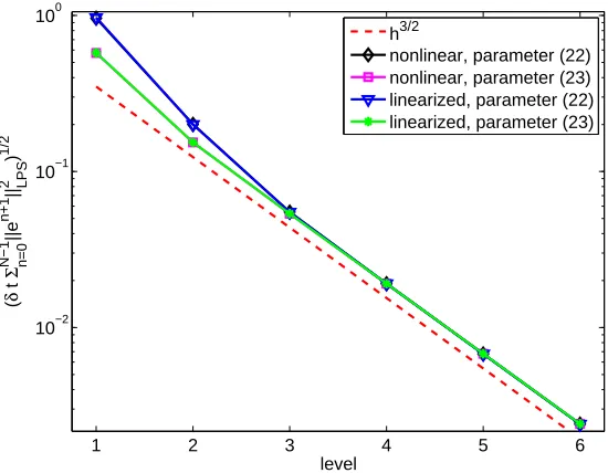
Remark. Theorems 9 and 10 prove the convergence of the method in the LPS norm plus an extra term involving the crosswind derivative of the error. Hence, these estimates give, essentially, an extra control of the whole gradient of the error.
4. The time-dependent problem
We now move on to the study of the time-dependent problem (3). A weak form of problem (3) reads as follows: Find u ∈ L2(0, T;H1(Ω)) ∩ H1(0, T;L2(Ω)) such that u = ub on [0, T]×∂Ω, u(0,·) = u0 and
(62) (ut, v) +a(u, v) = (f, v) ∀ v ∈H01(Ω), for almost every t∈(0, T].
To avoid technicalities in the analysis, it is assumed that the boundary condition does not depend on time, ub(t,·) = ub. The initial condition u0 is assumed to satisfy u0|∂Ω =ub and it is approximated by a function u0
h ∈Wh such thatu0h−ubhe ∈Vh.
To perform the discretization of the time derivative, the time interval [0, T] is divided into NT equidistant strips of length δt = T /NT. The constant time step is used only for simplicity of presentation; for variable time steps the same techniques can be applied leading to essentially the same results. The nodes are denoted by tn=n δt forn = 0,1, . . . , NT and
the abbreviations un :=u(tn,·), fn := f(tn,·), etc. are used. Since this section studies the
LPS method with nonlinear crosswind diffusion in combination with a one-step θ-scheme as temporal discretization, from now on, the superscript n+θ denotes for all functions which are defined in [0, T] the values at timetn+θ :=θ tn+1+ (1−θ)tn with anyn ∈ {0, . . . , NT−1}
and θ ∈ [0,1], e.g. bn+θ = b(tn+θ,·). For functions, which are defined only at the discrete
timestn andtn+1, it denotes the linear interpolation, e.g. un+θ
h =θ unh+1+ (1−θ)unh. Finally,
it is convenient to introduce the interpolation operator ˜rnh+θ satisfying
(63) ˜rnh+θu=θ rhun+1+ (1−θ)rhun
with rh from (43). Thus, writing α instead of n+θ, functionsuα, uαh, ˜rhαu, etc. are defined
Then, given θ∈(0,1], the fully discrete problem reads as follows: Forn = 0,1, . . . , NT−1, find unh+1 ∈Wh such that uhn+1−ubhe ∈Vh and
un+1
h −unh δt , vh
+an+θ(unh+θ, vh) +snh+θ(uhn+θ, vh) +dnh+θ(uhn+θ;unh+θ, vh) (64)
= (fn+θ, vh) ∀ vh ∈Vh.
For θ = 1/2, the Crank–Nicolson scheme is recovered and for θ = 1, the implicit Euler scheme is obtained.
Remark. To simplify the notation, we will not explicitly indicate at which time instant the functionsb andσ in the definition of the norm k · k
LPS are evaluated. This will be implicitly determined from the context or by the argument of the norm. Thus, if we write, e.g., kunh+θkLPS, the norm k · kLPS is defined using b
n+θ
and σn+θ.
4.1. Well-posedness and stability. The well-posedness of (64) can be traced back to the well-posedness of the LPS scheme with crosswind diffusion for the steady-state problem. The discretization of the temporal derivative can be written in the form
unh+1−un h δt , vh
= 1
θ
unh+θ−un h δt , vh
.
The first part of this term has the form of a reaction term for unh+θ. Thus, given un h, the
equation at the discrete time tn+1 is an equation for un+θ
h which has the same form as (19)
with the data of the problem attn+θ and with a reaction coefficient which has a contribution
from the temporal derivative. Thus, defining the operator ˜Thn+θ :Vh →Vh by
( ˜Thn+θzh, vh) = (Thn+θzh, vh) + 1
θ δt(zh +ubh, vhe )−
1
θ δt(u n
h, vh) ∀ zh, vh ∈Vh,
it follows that ˜Thn+θ(uhn+θ−uebh) = 0. Therefore, the existence and uniqueness of a solution unh+θ can be proved in the same way as in the steady-state case, see Section 3.1. This fact is stated in the next result.
Corollary 11. Let n∈ {0,1, . . . , NT −1} and un
h ∈Wh with unh|∂Ω =ubhe be given. If τM˜ is defined by (22) or (23), then the problem (64) possesses a solution unh+1. In the case thatτM˜ is defined by (22), the solution of (64) is unique. Furthermore, there is a constantC >0such that the solution of the scheme (64) withτM˜ given by (23) is unique ifδtkbn+θk
0,∞,M ≤C hM
for any M ∈Mh.
Proof. The only point remaining to prove is the uniqueness in the case ˜τM is given by (23).
norm by theL2(M) norm (10), (16),kPn+θ
M k2 = 1, and the inverse inequality (8), one arrives at
|dnh+θ(vh;vh, zh)−dnh+θ(wh;wh, zh)| ≤C X M∈Mh
h−1
M kbn+θk0,∞,Mkzhk20,M.
Thus, if vh, wh ∈Vh, one obtains
( ˜Thn+θvh−T˜hn+θwh, zh)≥ X
M∈Mh ˜
C θ δt −
Ckbn+θk
0,∞,M hM
!
kzhk20,M+kzhk2LPS.
Consequently, for δt small enough, the operator ˜Thn+θ is strongly monotone and hence the
solution to the discrete problem (64) is unique.
The next result states the stability of the method.
Lemma 12. Let θ ∈ [1/2,1] be given. Let ueα
h := uαh −eubh for any α ∈ [0, NT]. Then any
solution of (64) satisfies the following stability estimate for all N = 1,2, . . . , NT:
kueN
hk20,Ω+ (2θ−1)
N−1
X
n=0
keun+1
h −uenhk20,Ω+δt
N−1
X
n=0
keun+θ h k2LPS (65)
+δt N−1
X
n=0
dhn+θ(¯uhn+θ;eunh+θ,uenh+θ)≤ keu0hk20,Ω+C δt
N−1
X
n=0
n
σ0−1kfn+θk20,Ω
+hε+σ−1
0 (kbn+θk20,∞,Ω+kcn+θk20,∞,Ω) +hkbn+θk0,∞,Ω
i
keubhk21,Ω+µho,
where
¯
unh+θ =euhn+θ, µh =β hkbn+θk
0,∞,Ω|ubhe |13,3,Ω if τM˜ is given by (22),
(66)
¯
uhn+θ =uhn+θ, µh = 0 if τM˜ is given by (23).
(67)
Proof. The proof starts in the usual way by setting vh =uenh+θ ∈ Vh in (64) and using that
unh+1−un
h =eunh+1−uenh, which leads to
(uenh+1−eunh,euhn+θ) +δtkeunh+θk2
LPS+δt dnh+θ(unh+θ;unh+θ,eunh+θ)
(68)
=δt(fn+θ,euhn+θ)−δt an+θ(ubh,e eunh+θ)−δt shn+θ(eubh,eunh+θ).
A straightforward computation gives
(69) (eunh+1−uenh,eunh+θ) = 1 2(keu
n+1
h k
2
0,Ω− kuenhk20,Ω) +
2θ−1 2 keu
n+1
Next, the application of the Cauchy–Schwarz inequality, the Young inequality, (16), (18), the definition ofτM (20), and the geometrical hypotheses (4) and (5) yield
(fn+θ,uenh+θ)≤ 1
σ0 k
fn+θk20,Ω+1 4keu
n+θ h k
2 LPS,
an+θ(eubh,uehn+θ)≤6ε+σ−1
0 (kbn+θk20,∞,Ω+kcn+θk20,∞,Ω)
keubhk21,Ω+1 8kue
n+θ h k
2 LPS,
shn+θ(eubh,uehn+θ)≤C hkbn+θk
0,∞,Ω|ubhe |21,Ω+ 1 8keu
n+θ h k
2 LPS.
If ˜τM is given by (22), then, from (27) and an analog of (51), one obtains
dhn+θ(unh+θ;uhn+θ,uenh+θ)≥ 1 7d
n+θ
h (uenh+θ;uehn+θ,uehn+θ) +dnh+θ(eubh;ubh,e eunh+θ)
≥ 1
10d
n+θ
h (eunh+θ;uehn+θ,euhn+θ)−2dnh+θ(eubh;ubh,e ubhe ).
Furthermore, the use of (10), (16), (18), kPMn+θk2 = 1, (4), and (5) leads to
dnh+θ(ubhe ;ubh,e eubh)≤C β X M∈Mh
h1M−d/2kbn+θk
0,∞,M|ubhe |13,M ≤C β h˜ kbn+θk0,∞,Ω|ubhe |31,3,Ω.
If ˜τM is given by (23), then, using an inequality like (58), one gets
dhn+θ(unh+θ;unh+θ,uenh+θ) =dhn+θ(unh+θ;uenh+θ,euhn+θ) +dnh+θ(unh+θ;eubh,uenh+θ)
≥ 1
2d
n+θ h (u
n+θ h ;eu
n+θ h ,ue
n+θ h )−
1 2d
n+θ h (u
n+θ
h ;eubh,ubhe ).
Applying the H¨older inequality, (24), the estimate of the Lp(M) norm by the L2(M) norm (10), (16), kPMn+θk2 = 1, (4), and (5), one deduces that
dnh+θ(uhn+θ;ubh,e eubh)≤C X M∈Mh
h1+Md/2kbn+θk
0,∞,MkκM(PMn+θ∇eubh)k20,4,M
≤C h˜ kbn+θk
0,∞,Ω|eubh|21,Ω.
Now, inserting the above relations into (68) and using the notation (66) and (67), one obtains 1
2(kue
n+1
h k
2
0,Ω− keunhk20,Ω) +
2θ−1 2 kue
n+1
h −eu n hk20,Ω+
δt
2 keu
n+θ h k
2 LPS+
δt
6 d
n+θ h (¯u
n+θ h ;eu
n+θ h ,ue
n+θ h )
≤δt σ0−1kfn+θk2
0,Ω+C δt
ε+σ0−1(kbn+θk2
0,∞,Ω+kcn+θk20,∞,Ω) +hkbn+θk0,∞,Ω keubhk21,Ω
+C δt µh,
and (65) follows by summing up from n = 0 toN −1.
Remark. The inequality (65) is a proper stability result provided thatku0
hk0,Ω,kubhe k1,Ω and, if ˜τM is given by (22), also |uebh|1,3,Ω are bounded when h→ 0. One may set u0h =Ihu0 and
e
and eub ∈ H1(Ω) is an extension of ub. Then ku0
hk0,Ω ≤ Cku0k1,Ω and kubhe k1,Ω ≤Ckubek1,Ω. If ube ∈W1,3(Ω) (requiring the stronger assumption ub ∈ W2/3,3(∂Ω)), then also |ubhe |
1,3,Ω ≤
Ckeubk1,3,Ω. It is important thatIh preserves homogeneous boundary conditions since one has to assure thatu0
h and eubh coincide on the boundary of Ω. Ifu0 ∈H2(Ω) and ub ∈H3/2(∂Ω), which are the minimal regularity assumptions for deriving the error estimates in the next section, one may use the operator ih from Section 2 instead of Ih. Now ube ∈ H2(Ω) and, according to the approximation properties of ih (11) and (13), one has ku0
hk0,Ω ≤Cku0k2,Ω and kubhe k1,Ω+|ubhe |1,3,Ω ≤Ckeubk2,Ω.
Remark. It is worth remarking that, for the homogeneous caseub = 0, instead of the direct proof presented in this manuscript, an analysis completely analogous to the one given in [8], Corollary 7, leads to the following stability result for θ ∈[1/2,1] andN < NT
1 2ku
N
h k20,Ω+δt
N−1
X
n=0
kunh+θk2
LPS+dnh+θ(uhn+θ;unh+θ, unh+θ)
(70)
≤ eT−δtT
(
T δt N−1
X
n=0
kfn+θk2 0,Ω+
1 2ku
0
hk20,Ω
)
.
This result, very similar in form to the one in [8] (with the extra control on the nonlinear term, and a slightly smaller right-hand side), is independent of σ0, and hence represents an improvement over the way Lemma 12 is presented. The reason to present the direct proof here lies in the non-homogeneous case, where the presence ofub is responsible for the
dependency of the constant on the right-hand side on σ0−1. In the non-homogeneous case, both proofs lead to essentially equivalent results, the direct proof presented in this work being more straightforward.
Finally, if ub would be supposed time dependent, then in the first line of the proof of
stability there holds unh+1−un h =ue
n+1
h −eunh+eu n+1
bh −uenbh, thus creating an extra right-hand
side depending on the time derivative of ub.
4.2. Error estimates. In this section, error estimates are derived for the solution of the discrete problem (64) withθ ∈[1/2,1]. The error will be analyzed essentially in the quantity which is given by the stability estimate (65). Let us denote the error by eα := uα −uα h
quantities
EN =keNk0,Ω+ δt
N−1
X
n=0
ken+θk2 LPS
!1/2
,
QN =h|u0|k+1,Ω+|uN|k+1,Ω+σ
−1/2
0 kutkL2(0,tN;Hk+1(Ω))
+ δt N−1
X
n=0
ε+hkbn+θk
0,∞,Ω
+h2kσn+θk0,∞,Ω+h2σ
−1
0 |bn+θ|21,∞,Ω
|un|2k+1,Ω+|un+1|2k+1,Ω
!1/2
,
RN = δt N−1
X
n=0
hk+1−d/2kbn+θk
0,∞,Ω
|un|3
k+1,Ω+|un+1|3k+1,Ω
!1/2
,
SN = δt NX−1
n=0
hk+1kbn+θk
0,∞,Ω
|un|k+1,∞,Ω+|un+1|k+1,∞,Ω
|un|2
k+1,Ω+|un+1|2k+1,Ω
!1/2
,
XN = max
n=0,...,N−1 ε+hk
bn+θk
0,∞,Ω+kσn+θk0,∞,Ω+σ
−1
0 kbn+θk20,∞,Ω+σ
−1
0 kcn+θk20,∞,Ω
1/2
,
YN =h1/2 max
n=0,...,N−1 k
bn+θk1/2
0,∞,Ω,
where N = 1,2, . . . , NT.
Theorem 13. Let θ ∈ [1/2,1] be given. Let the weak solution of (3) satisfy u, ut ∈ L2(0, T;Hk+1(Ω))for some k∈ {1, . . . , l}and assumeutt ∈L2(0, T;L2(Ω)). Let eub ∈H2(Ω) be an extension of ub and let eubh = ihube. Assume u0 ∈ Hk+1(Ω) and let u0h = ihu0. Let
{un h}
NT
n=0 be the solution of the local projection discretization (64). If τ˜M is defined by (22)
and ut∈L3(0, T;W1,3(Ω)), then the error estimate
EN + δt N−1
X
n=0
X
M∈Mh ˜
τMkκM(PMn+θ∇en+θ)k3 0,3,M
!1/2 (71)
≤C hkQN +C β hkRN +C δt XNkutkL2(0,tN;H1(Ω))
+C β(δt)3/2YNkutkL3/32(0,tN;W1,3(Ω))+C δt σ
−1/2