City, University of London Institutional Repository
Citation:
Broom, M. and Rychtar, J. (2008). An analysis of the fixation probability of a
mutant on special classes of non-directed graphs. Proceedings of the Royal Society A:
Mathematical, Physical and Engineering Sciences, 464(2098), pp. 2609-2627. doi:
10.1098/rspa.2008.0058
This is the unspecified version of the paper.
This version of the publication may differ from the final published
version.
Permanent repository link:
http://openaccess.city.ac.uk/979/
Link to published version:
http://dx.doi.org/10.1098/rspa.2008.0058
Copyright and reuse: City Research Online aims to make research
outputs of City, University of London available to a wider audience.
Copyright and Moral Rights remain with the author(s) and/or copyright
holders. URLs from City Research Online may be freely distributed and
linked to.
City Research Online:
http://openaccess.city.ac.uk/
[email protected]
mutant on special classes of non-directed
graphs
B y M. Broom1 and J. Rycht´aˇr2 †
1 Department of Mathematics, University of Sussex, Brighton BN1 9RF, UK
2 Department of Mathematics and Statistics, University of North Carolina
Greensboro, NC27402, USA
There is a growing interest in the study of evolutionary dynamics on populations with some non-homogeneous structure. In this paper we follow the model of
Lieber-manet al. [Lieberman, E., Hauert, C., Nowak, M.A. 2005 Evolutionary dynamics
on graphs.Nature43(3), 312–316] of evolutionary dynamics on a graph. We
inves-tigate the case of non-directed equally weighted graphs and find solutions for the fixation probability of a single mutant in two classes of simple graphs. We further demonstrate that finding similar solutions on graphs outside these classes is far more complex. Finally we investigate our chosen classes numerically, and discuss a number of features of the graphs; for example we find the fixation probabilities for different initial starting positions and observe that average fixation probabili-ties are always increased for advantageous mutants as compared against those of unstructured populations.
Keywords: Evolutionary dynamics, star, linear graph, random walk, Markov chain
1. Introduction
Evolutionary dynamics models are widespread, but have generally assumed homoge-neous populations. The study of evolutionary dynamics on graphs was investigated in the paper Liebermanet al.(2005), other important work on this subject being in Erd¨os & Renyi (1960); Nagylaki & Lucier (1980); Barabasi & Albert (1999). Each vertex or node represents an individual in the population, and individuals can re-produce into neighbouring vertices, i.e. those connected by an edge. In Lieberman
et al. (2005) at each stage an individual was selected randomly, with probability
proportional to its fitness, which then copied itself into one of the vertices it was connected to. (It should be noted that there are other possible dynamics. An ex-ample is the biased voter model, e.g. see Bramson & Griffeath (1981), where an individual is chosen at random to be removed and is replaced by a copy of one of its neighbours). Liebermanet al. (2005) considered directed graphs where con-nections between vertices can be one-way only (e.g. it is possible for an individual at 1 to reproduce into 2, but not for one at 2 to reproduce into 1), with general weightings indicating the probability that any particular vertex would be replaced, given the chosen replacing vertex. They showed several interesting and important
results; for instance, different graph structures could yield different probabilities for fixation of a single mutant. In homogeneous populations the probability of fixa-tion in a populafixa-tion withN individuals (and soN vertices) is given by the Moran probability
PM oran=
1−1/r
1−1/rN (1.1)
where resident individuals have baseline fitness 1 and mutants have fitnessr(each individual being chosen as the reproducing individual with probability proportional to its fitness). It was shown in Liebermanet al. (2005) that this probability holds under a condition on the weightings on the graph, any graph satisfying this con-dition being referred to as an isothermal graph. However, other graph structures allow the probability of fixation of an advantageous mutant (r >1) to converge to either 0 or 1 asN tends to infinity.
Most of the interesting results from Lieberman et al. (2005) relied on graphs being directed and the weights of connections from a given vertex to be different from each other. In this paper we look at non-directed graphs with equal weights. We show that in this setting, the formula (1.1) holds for regular graphs, graphs where every vertex has the same degree, and only for them. We then show that evolutionary dynamics on a graph withNvertices leads to a system of 2Nequations;
with the exception of a circle (a regular graph case) and a line (a non-regular graph). We use symmetries to reduce the number of equations to 2n+ 1 for a star with
N =n+ 1 vertices. In Lieberman et al. (2005), the approximation of the fixation probability for stars for largenwas given by
P = 1−1/r
2
1−1/r2n (1.2)
Here we find the exact fixation probabilities for anyrandn.
We then analyze the dynamics on the line. The analysis is quite hard to perform even in this simple case, although we make substantial progress. We also make suggestions about how to attack the more general problem without simply resorting to numerical methods and simulation.
2. Evolutionary dynamics on graphs
LetG= (V, E) be a finite, undirected and connected graph, whereV is the set of vertices andEis the set of edges. We assume that the graph is simple, i.e. no vertex is connected to itself. We study evolutionary dynamics as described in Liebermanet al.(2005), see also Nowak (2006). We treat the dynamics as a discrete time Markov chain. At the beginning, a vertex is chosen uniformly at random and replaced by a mutant with fitnessr, all remaining vertices having fitness 1.
If the mutants already inhabit precisely the vertices in the setC ⊂V, then in the next step the mutants will inhabit vertices in either
1) a set C∪ {j},j6∈C, provided a) a vertexi∈C was chosen for reproduction and b) it placed its offspring into vertexj; or
3) a set C, provided an individual from C (V \C) replaces another individual fromC (V \C).
The states ∅ and V are the absorbing points of the dynamics. The transition probabilities of the above Markov chain are determined by a) the probability that a given vertex will be selected for reproduction and b) the probability that, once selected, it places its offspring into another given vertex.
We set the fitness of an individual at vertexiasfi∈ {1, r}, wherefi=rmeans
that the individual is a mutant. An individual atiis selected for reproduction with probability
si=
fi
P
j∈V fj
. (2.1)
The graph structure is represented by a matrix W = (wij), where wij is the
probability of replacing a vertex j by a copy of a vertexi, provided vertex iwas selected for reproduction,
wij=
(1
ei, ifi andj are connected,
0, otherwise,
whereei is the number of edges incident to the vertexi, so that edges have equal
weights.
LetPCdenote the probability of mutant fixation given mutants currently inhabit
a setC. The rules of the dynamics yield, see Liebermanet al. (2005),
PC =
X
i∈C
X
j6∈C
rwijPC∪{j}+wjiPC\{i}
rX
i∈C
X
j6∈C
wij+
X
i∈C
X
j6∈C
wji
(2.2)
withP∅= 0 andPV = 1.
This system has a unique solution following from the uniqueness of a Markov chain given a known initial distribution. There is a unique distribution over the states at time 0 (a single mutant is introduced to the population at a randomly chosen vertex). The Kolmogorov equations then give a unique distribution at step
s+ 1 conditional on uniqueness at steps. As s tends to infinity, there is conver-gence to the set of absorbing states (either all mutants or all residents). This yields a unique limiting distribution, so a unique fixation probability from the initial dis-tribution.
The system (2.2) of linear equations is very large (typically of the order of 2|V|
equations, see §4) and very sparse (from any stateC, one can go to at most |V|
other states).
3. Regular graphs
A graph is called isothermal if P
jwji is constant as a function of i. A graph is
isothermal if and only if the matrixW = (wij) is double stochastic (Lieberman et
al., 2005), i.e.
X
j
It is proved in Liebermanet al. (2005) that if a graph is isothermal then
PC=
1− 1 r|C|
1− 1 r|V|
(3.1)
Here we give a different proof of this statement and one more equivalent condition to being isothermal.
Theorem 3.1. A simple connected undirected graph G= (V, E) is isothermal if
and only if it is regular.
Proof. Clearly, ifGis regular,eiis constant, and thusGis isothermal. Now suppose
that the relation in the other direction is not true. Consider a set C = {i, ei =
min{ev, v∈V}}. Since, by our assumption,C 6=V, there must be a vertex i∈C
that is connected to a vertexj∈V \C. Then,
X
v
wvi =wji+
X
v6=j
wvi<
1
ei
+X
v6=j
wvi≤
1
ei
+ei−1
ei
= 1,
a contradiction.
In order to solve (2.2) for an isothermal graph, let us assume that PC only
depends upon the size ofC, so that
PC=x|C|. (3.2)
By theorem 3.1,wij attains only one nonzero value (1/k, where kis the degree of
any vertex inG) and thus (2.2) reduces to
x|C|= r
r+ 1x|C|+1+ 1
1 +rx|C|−1. (3.3)
This is a standard difference equation that gives the required Moran probabili-ties. Consequently, our assumption (3.2) leads to a solution of (2.2) and by the uniqueness of the solution, the solution must satisfy the property (3.2).
4. Complexity of the dynamics
Since at every vertex of a graph G = (V, E) there can be either a resident or a mutant, there are up to 2|V| potential mutant formations and thus up to 2|V|
equations in (2.2).
Some formations of mutants on a given graph are identical because of symme-tries (automorphisms) of the graph. Certain graphs (like a complete graph, or a star graph - see§5) thus have only a few possible mutant-residents patterns since their automorphisms group is very rich. For other graphs, like a line, the graph structure itself yields only symbolic reduction of the number of patterns because the automorphism group consists of only a few nontrivial elements.
of possible formations. Consider the setX consisting of all possible 2|V|
mutant-residents patterns. Forf ∈Aut(G), let Fix(f) ={v∈V, f(v) =v}. If Fix(f)6=V, thenffixes 2|Fix(f)|+1elements ofX(one has freedom to put a mutant or a resident
in any vertex v ∈Fix(f), plus one can place either mutants or residents into all vertices ofV \Fix(f)). Clearly, identity on Gis the onlyf ∈Aut(G) that fixes all elements ofG. Burnside’s theorem then yields the total number of Mutant-Resident Formations (MRF) ofGas
MRF(G) = 1
|Aut(G)|
2|V|+
X
f∈Aut(G),f6=idG
2|Fix(f)|+1
(4.1)
The above considered the graph structure only, not considering the rules of the dynamics at all. Clearly, any non-initial state of the dynamics contains at least one parent-offspring pair of connected vertices. Consequently, alternating patterns, i.e. patterns where any pair of connected vertices is inhabited by a mutant at one vertex and a resident an the other vertex, cannot be attained as a result of the dynamics. Alternating patters are possible if and only if the graph does not contains an odd cycle (i.e. if the graph is bipartite). There are at most 2 alternating patterns.
On a circle or on a line, any mutant formation resulting from the dynamics consists of a connected segment. Hence, there are of the order of|V|2 patterns on
a circle (|V|possibilities where the segment starts and|V| −1 possibilities where it ends, plus the patterns with all or no mutants) and|V|2/2 patterns on a line (|V|
possibilities to start, and on average|V|/2 possibilities where the segment can end). Moreover, the rotations on the circle help us to reduce the number of equations to
|V|; the symmetry of a line also reduces the number of equations by a factor 1/2 to approximately|V|2/4.
The next theorem shows that for the vast majority of graphs, the system (2.2) consists of roughly MRF(G) equations.
Theorem 4.1. If a graph contains a vertex of degree at least 3 (i.e. the graph is
neither a line nor a circle), and the dynamics is in any non-absorbing state, then there is a nonzero probability that the dynamics will evolve to any of the possible
MRF(G)states (MRF(G)−2states if the graph is bipartite).
Before proving theorem 4.1, we prove a result required for the proof.
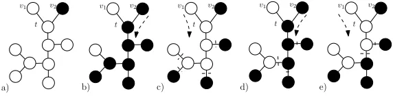
Lemma 4.2. Let verticesv1andv2be connected to a vertext. Furthermore, assume
that there is a mutant in v2 and resident in v1. Then, we can fill any pattern to
any subtree structure connected to tand not containingv1 andv2.
Proof of lemma 4.2. The proof goes by the induction on the height of the subtree
structure. If the height is 1 (i.e. the structure is only the vertext), we can clearly fill it by a mutant or a resident. Now assume that we can fill any pattern to the subtree of heightn−1 and that our structure has a heightn.
First, spread the residents (from v1) to get the structure which contains only
residents, see figure 1a). Next, spread the mutants (fromv2) to every vertex but
v1 v
2
t
v
1 v2
t
v1 v
2
t
v
1 v2
t
v
1 v2
t
[image:7.612.143.429.83.153.2]a) b) c) d) e)
Figure 1. Filling a given pattern (figure e)) to a subtree connected tot. The original configuration is a) - a mutant inv2 and a resident inv1.
Proof of theorem 4.1. We now prove theorem 4.1 using multiple applications of
lemma 4.2. To do this, there are some technical difficulties that has to be overcome. Firstly the original graph has to be ”trimmed” to become a tree so we can apply the lemma. Secondly we need a ”manoeuvring” space since the lemma 4.2 does not allow us to fill patterns ”behind” the verticesv1 andv2, and thus we need to
arbitrarily flip the roles of vertices connected tot. We obtain this space by collapsing the target pattern by a single vertex, which allows us to have the central vertex completely free for our use. Finally, the trimming could cause some patterns to become inaccessible (alternating) on the tree, although they were not alternating on the original graph, so we will have to deal with these patterns in one more step. Firstly we trim the graph to get a tree. Denote the vertex of degree at least 3 by
t0 and label three of its neighbours byt1, t2, t3. Next, trim the graph by cutting a
sufficient number of edges to get a connected tree (a graph with no cycle) consisting of all of the original vertices and yet keeping all of the edgest0tj, i= 1,2,3 intact.
Label the remaining neighbours (if any) oft0 by t4, . . . , tk. We will show that we
can reach any state that is non-alternating (on this tree) from any non-absorbing state even if only the edges of this trimmed graph are used.
Secondly we collapse a pattern to get the central vertext0 for free usage. Since
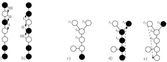
the target state is not alternating, there are two connected vertices with the same type of inhabitants. We may assume that the vertices are on the branch (linear set)
B=b0b1b2b3· · ·blwithb0=t0andb1=t1; letbiandbi+1be the two vertices with
the same inhabitants and with the lowest indexipossible. LetS denote the target state andS∗ the state that is the same as the target state except that at vertices bj, j = 1,· · ·, iit has inhabitants from the vertices bj−1 of the target state. Note
that S andS∗ are each attainable from the other by a shift of the pattern along
the line. See figure 2a) and 2b) for an illustration of this.
We now move the mutants into a position where lemma 4.2 can be applied. From above it is enough to reach the stateS∗. Also, we may assume that inS∗, t1 is inhabited by a mutant (i.e. in the original target state, t0 is inhabited by a
mutant). If the contrary is true, we would just interchange the role of residents and mutants in the following arguments.
Clearly, any non-absorbing state can evolve into a state with one mutant only. If the mutant is not att2already, we can relabelt2andt3such that the shortest path
from the mutant’s position tot2goes throught0. Now the mutants can spread tot2
I. II. III
I.
II.
III.
a) b)
t1 t2
t0
t3
t1 t2
t0
t3
t1 t2
t0
t3
c) d) e)
Figure 2. a) and b) Shifting between patterns on the line. c), d) and e) Moving a single mutant from a general position tot2.
Applying lemma 4.2 for the first time, we can fill any pattern to subtrees starting att3, t4,· · · , tk by lemma 4.2.
We now rotate the mutant-resident pattern aroundt0and fill the branch behind
vertext1; then rotate again and fill behindt2. We use lemma 4.2 to place a resident
att3(thus having a mutant att2and resident att3) and use lemma 4.2 again to fill
the patternS∗ to the subtree starting att
1. At the end, there will be a mutant in t1. Since now we have a mutant int1 and a resident int3, we can fill the required
pattern to the subtree starting at t2. If there has to be a mutant at t3, place it
there by spreading fromt1 throught0. In any case, finish by shifting the pattern
fromS∗ toS.
So far, we were able to reach any state that is not alternating on the trimmed graph. It is possible that an alternating state on the trimmed graph is not an alternating state on the original graph. If we want to reach this pattern, let us pick verticesw1, w2witnessing that the pattern is not alternating on the original graph.
We may assume that they are both inhabited by mutants. If we change the mutant inw1into a resident, we get a pattern that is not alternating on the trimmed graph.
In particular, we can reach it as shown above. And to reach the required pattern, it only remains to spread the mutant from w2 into w1 - we can do that because
verticesw1 andw2 are connected in the original graph.
5. Dynamics on stars
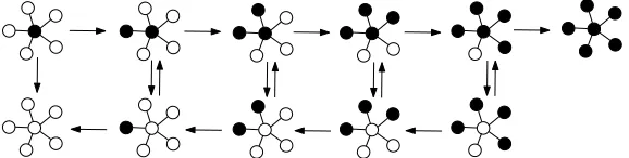
In this section we consider a star - a non-directed graph with N =n+ 1 vertices labeled 0,1, . . . , nwhere the only edges are between vertices 0 and i,i= 1, . . . , n. The vertex 0 is called a centre and the vertices 1, . . . , n can be called the leaves. The automorphism group is isomorphic to the group of permutations on leaves and the state of the dynamics can be described by the number of mutants at the leaves and by an indicator of whether or not there is a mutant at the centre. See figure 3 for a scheme of the dynamics. LetP0
i (Pi∅, respectively) denote the probability
[image:8.612.145.427.80.186.2]Figure 3. States of a dynamics on a star withn= 5 leaves.
P0
i =
r r+nP
0
i+1+ n r+nP
∅
i (5.1)
Pi∅ =
nr nr+ 1P
0
i +
1
nr+ 1P
∅
i−1 (5.2)
fori= 0, . . . , n with boundary conditionsP∅
0 = 0 and Pn0 = 1. The equation (5.1)
can be rearranged to
Pi0=P
0
i−1+ n r(P
0
i−1−Pi∅−1) (5.3)
We can use (5.3) and (5.2) to inductively calculateP1∅, P20, P2∅, . . . as a function of P0
1 to get
P0
i =P10·
1 + n n+r
i−1 X
j=1
n+r r(nr+ 1)
j
SincePn0= 1, we get
P10=
1
1 + n n+r
Pn−1
j=1
n+r r(nr+1)
j
Since, by (5.1) and (5.2),
P00 = r r+nP
0 1
P1∅ = nr nr+ 1P
0 1
we get that the average fixation probability for a mutant is
%= n
nr nr+1+
r r+n
(n+ 1)·
1 + n n+r
Pn−1
j=1
n+r r(nr+1)
j
Notice that for largenwe get
%≈ 1
1 +Pn−1
j=1 r12j
= 1−
1
r2
1− 1
r2n
a) 0.35 0.4 0.45 0.5 0.55
20 40 60 80 100
n b) 0.2 0.4 0.6 0.8 1
2 4 6 8 10
[image:10.612.125.436.91.190.2]r
Figure 4. The mean fixation probability for a star (middle curve) and comparison to
PM orangiven in (1.1) (lowest curve) and formula (1.2) (upper curve). This comparison is
shown in a) for a range of values ofnandr= 1.5, and in b) for a range of values ofrand
n= 10.
1/2 r+1/2 r r+1/2 1 r+1 1 r+1 1 r+1 1 r/2+1 r r+1 r r+1 r
r+1 r/2+1r/2
r/2 r+1 r/2 r+1 r/2 r+1 r/2 r+1 r/2 r+1 r/2 r+1 r/2 r+1 r/2 r+1 r/2 r+1 r/2 r+1 r/2 r+1 r/2 r+1 1/2 r+1 1/2 r+1 1/2 r+1 1/2 r+1 1/2 r+1 1/2 r+1 r/2 r+1 r/2 r+1 r/2 r+1 1/2 r+1 1/2 r+1 1/2 r+1 1/2 r+1 r/2 r+1 r/2 r+1 r/2 r+1 1/2 r+1 1/2 r+1 1/2 r+1 1/2 r+1 1/2 r+1 1/2 r+1 1/2 r+1 1/2 r+1
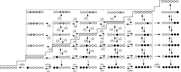
Figure 5. States of a dynamics on a line with n+ 1 = 6 vertices (below the “stairs”). The larger rectangle represents where the dynamics will be extended in§6d. The dotted arrows represent fictional transitions that will be used for the extension. The states on the boundary of the larger rectangle are absorbing states of the fictional extension. The smaller rectangle shows the states where the transitions depend on the direction only and not on the actual state. The black circles represent mutants. The lines with grey circles represent the fictional states [i, j) for j > i.
6. Dynamics on lines
[image:10.612.108.466.269.413.2](a) States and transition probabilities
The mutant population starts with a single individual; new mutants can only arise in vertices on neighbouring points on the line, and mutants can only be lost from vertices connected to a resident individual. Thus the population of mutants forms a line segmenti, i+ 1, . . . , j−1 for some pair (i, j) wherei≤j, and the state of the system can be described by this pair of numbers only. The evolution of the population can thus be seen as a 2-d random walk on a triangular set
T ={(i, j),0≤i≤j≤n+ 1}.
Let Pi,j denote the probability of mutant fixation given that we are at the state
(i, j). Once the population reaches the diagonal state (i, i) for 0≤i≤n+ 1, the mutants are extinct, i.e.
Pi,i= 0. (6.1)
Once a mutant reaches an end vertex, i.e. the population is in the state (0, j) or (j, n+ 1) for some 0 ≤ j ≤n+ 1, it will never be removed from the end vertex unless through extinction, since it can only be removed by a resident on its sole neighbouring vertex, which in turn can only be present if the end vertex individual is the sole mutant in the population. Hence, the population stays on these boundary lines once it reaches them. In§6bwe calculate that
P0,j =Pn+1−j,n+1=2r
n+1−rn−rn+1−j
2rn+1−rn+r−2 . (6.2)
We thus have to solve the 2-dimensional random walk on a set T given the boundary conditions (6.1) and (6.2).
We proceed to investigate the transitions in the interior ofT. First, it should be noted that for most choices of a vertex for reproduction, the population does not change. The only change occurs when we choose a vertex on a boundary between mutants and non-mutants. When 2≤i < j ≤n−1, there are two boundaries and a change of state may occur if any of the verticesi−1, i, j−1 orjare chosen. None of these vertices is an end vertex and thus
Pi,j=
r
2(r+ 1)Pi−1,j +
r
2(r+ 1)Pi,j+1+ 1
2(r+ 1)Pi+1,j + 1
2(r+ 1)Pi,j−1. (6.3)
When a mutant occupies one of the end vertices, there is just one mutant-resident boundary, and only two choices of vertices allow a change of state.
P0,1 = r r+1
2
P0,2 (6.4)
P0,j =
r
r+ 1P0,j+1+ 1
r+ 1P0,j−1, 2≤j≤n−1 (6.5)
P0,n =
1 1 +r
2
P0,n−1+
r
2
1 + r
2
(6.6)
When a mutant occupies a vertex next to an end vertex (1 or n−1), with a resident at the corresponding end vertex we have, for 2≤j≤n−1,
P1,j = r
2
r+32P0,j+
r
2
r+32P1,j+1+
1 2
r+32P1,j−1+ 1
r+32P2,j, (6.8)
P1,n = r
2
r+ 2P0,n+
r
2
r+ 2P1,n+1+ 1
r+ 2P1,n−1+ 1
r+ 2P2,n, (6.9)
Pj,n = P1,n+1−j. (6.10)
The system (6.3)-(6.10) consists of the order ofn2/2 equations. By symmetry
(equations (6.7) and (6.10)), the system reduces to the order ofn2/4 equations.
(b) Boundary conditions
The equations (6.4), (6.5), and (6.6) are difference equations for P0,j. Using
standard methods (see e.g. Norris (1997, Chapter 1)), by (6.5), we have to find the roots of
−(r+ 1)x+rx2+ 1 = 0.
Since the roots arex= 1 andx=1r, we get
P0,j =A+B
1
r j
. (6.11)
The values A, B are determined after technical calculation using equations (6.4) and (6.6). This yields, for 0≤j≤n+ 1,
P0,j =Pn+1−j,n+1 =
rn+1−j+rn−2rn+1
2−r+rn−2rn+1
= rn+1−j 1 +r+· · ·+r
j−2+ 2rj−1
2 +r+r2+· · ·+rn−1+ 2rn. (6.12)
(c) The inner boundary
Using the equations (6.8), (6.9) and (6.10) we obtain
−r
2P1,j+1+
r+3
2
P1,j −
1
2P1,j−1 =
r
2P0,j +P2,j, (6.13) (r+ 2)P1,n−2P1,n−1 = rP0,n. (6.14)
Since we can calculateP0,j, j= 0, . . . , n, we just need to calculateP2,jin terms of
P1,k, k= 1, . . . , nto get a system ofnequations fornunknownsP1,k, k= 1, . . . , n.
(d) Interior points
In Miller (1994) a 2-d random walk on a square lattice
with arbitrary boundary conditions at states
(0, j),(n+ 1, j),(i,0),(i, n+ 1), 0≤i, j≤n+ 1
was solved. In this paper we relabel the boundary coordinates of the square to be appropriate to the application from our problem, giving
S={(i, j); 1≤i, j≤n}
with boundary conditions at states
(1, j),(n, j),(i,1),(i, n), 1≤i, j≤n.
Our goal is to extend the random walk from T onto S while giving fictional boundary conditions onS such that the restriction of the extended walk will give us exactly the original walk on T with the boundary conditions (6.1) and (6.2). This is illustrated in Figure 5.
In the notation of Miller (1994), we have
Pi,j =
1 2(r+ 1)
n−1 X
a=2 n
Pa,1T(a,2)ij + rP1,aT(2,a)ij+rPa,nT(a,n−1)ij
+ Pn,aT(n−1,a)ij
o
(6.15)
whereT(a,b)ij is the expected number of times the state (a, b) is visited given that
the initial state is (i, j). By Miller (1994, equation 4.3),
T(a,b)ij=r
i−a−j+b
2 f(a−1, b−1, i−1, j−1), (6.16)
where
f(a, b, i, j) = 4 (n−1)2
n−2 X
k,s=1
sinikπ n−1
sinakπ n−1
sinbsπ n−1
sinnjsπ−1
1−r√+1r hcos kπ n−1
+ cos sπ n−1
i .
Notice that
f(a, b, j, j) =f(b, a, j, j). (6.17)
(e) Fictitious boundary conditions
It should be noted that in this section we are not dealing with the fixation prob-abilities as such, but rather finding methods of solving an arbitrary set of equations. Thus we will have expressions in terms that resemble probabilities, but which are not (e.g.Pi,j wherei > j), which have negative solutions. These solutions however
obey the correct transition equations and have the correct boundary conditions for the region of interest.
In this section we give the fictitious boundary conditions for the random walk on the whole square. So far, in §6c we have equations for P1,a and Pa,n for all
1≤a≤n. We need to calculatePa,1 andPn,a. By (6.1), (6.15), (6.16), and (6.17)
0 = Pj,j
= 1
2(r+ 1)
n−1 X
a=2 n
f(a,2, j, j)hPa,1r 2−a
2 +P1,ar
a
+f(a, n−1, j, j)hPa,nr
n+1−a
2 +Pn,ar
a+1−n 2
io .
The above can be true if
Pa,1r 2−a
2 +P
1,ar
a
2 = 0,
Pa,nr
n+1−a
2 +Pn,ar
a+1−n
2 = 0.
This implies
Pa,1 = −ra−1P1,a,
Pn,a = −rn−aPa,n.
(f) Reduction to nequations
Denote
dx,yi,j=f(x, y, i, j)−f(y, x, i, j).
Consequently, by (6.10), (6.15) and (6.16),
Pi,j =
ri−j 2
2(r+ 1)
n−1 X
a=2 n
P1,ar
a
2di,j
2,a +Pa,nr
n+1−a
2 di,j
a,n−1 o
(6.18)
= r
i−j 2
2(r+ 1)
n−1 X
a=2 n
P1,ar
a
2di,j
2,a +P1,n−a+1r
n+1−a
2 di,j
a,n−1 o
. (6.19)
Referring back to (6.13) and (6.14), this gives us the following linear simultaneous equations in the probabilitiesP1,j, 2≤j≤n−1, andP1,n
r
2P0,j = −
r2−j 2
2(r+ 1)
n−1 X
a=2 n
P1,ar
a
2d2,j
2,a+P1,n−a+1r
n+1−a
2 d2,j
a,n−1 o
−r
2P1,j+1+
r+3
2
P1,j−
1 2P1,j−1
rP0,n = (r+ 2)P1,n−2P1,n−1.
After solving the above system forP1,k, we can reconstructPi,jfor alli, jby (6.19).
The fixation probability for a line is then given by
P[fix] = 1
n+ 1
n
X
i=0
Pi,i+1. (6.20)
7. A comparison between line and circle with a numerical
example
a)
0 0.1 0.2 0.3 0.4
Average Fixation Probability
10 20 30 40 50
Number of Vertices
b) 0
0.05 0.1 0.15 0.2 0.25 0.3
Average Fixation Probability
10 20 30 40 50
[image:15.612.134.435.76.179.2]Number of Vertices
Figure 6. Dependence of the average fixation probability for a line on the number of vertices (n+ 1) in the line; a)r= 1.1 , b)r= 0.9.
a)
0 0.001 0.002 0.003 0.004 0.005
Difference between Line and Circle 10 20 30 40 50 Number of Vertices
b) –0.005
–0.004 –0.003 –0.002 –0.001 0
Difference between Line and Circle
10 Number of Vertices20 30 40 50
c) 0
0.01 0.02 0.03 0.04 0.05
Relative Difference between Line and Circle
10 20 30 40 50
Number of Vertices d) –0.2 –0.18 –0.16 –0.14 –0.12 –0.1 –0.08 –0.06 –0.04 –0.020
Relative Difference between Line and Circle
10 Number of Vertices20 30 40 50
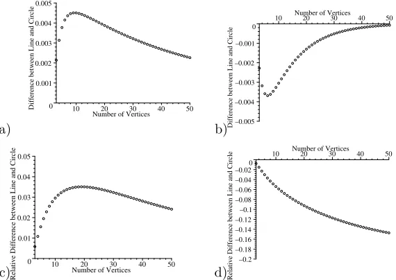
Figure 7. The difference between the average fixation probability for a line and for a circle (Moran process); a)r= 1.1, absolute difference (line-circle), b)r= 0.9, absolute difference, c)r= 1.1 relative difference (line-circle)/line, d)r= 0.9 relative difference.
mutants which are less fit. In figure 6, we can see how the average fixation proba-bility for a line decreases as the number of vertices increases. The decrease is much steeper forr <1. For anyr, the average fixation probability for a line approaches the Moran probability (demonstrated in figure 7). Ifr >1, the fixation probability for a line is greater than the fixation probability for the Moran process and it is smaller otherwise. Figure 8 shows how the absolute and relative difference changes asrchanges from 0 to larger numbers. The absolute difference is at its largest for mutants which are advantageous, but not overwhelmingly so. This is reasonable as these have an intermediate probability of fixation and so structural changes have the greatest possibility of altering this probability. Very advantageous mutants are likely to achieve fixation whatever the structure, and non-advantageous ones are unlikely to do so (note that the large relative difference for small r in figure 8b corresponds to a very small fixation probability in each case). The dependence of the difference between a line and a circle onr is more or less the same for othern
[image:15.612.141.426.222.424.2]a) –0.004
–0.0020 0.002 0.004 0.006 0.008 0.01 0.012 0.014
Difference between a Line and a Circle
1 2 r 3 4 5
b)
–0.7 –0.6 –0.5 –0.4 –0.3 –0.2 –0.1 0 0.1
Relative difference between a Line and a Circle
[image:16.612.138.426.91.191.2]1 2 r 3 4 5
Figure 8. The difference between the average fixation probability for a line and for a circle (Moran process) when there are 10 vertices; a) absolute difference (line-circle), b) relative difference ((line-circle)/circle).
a) 0
0.2 0.4 0.6 0.8 1
Fixation Probability
2 4 6 8 10
Vertex Number b) 0
0.02 0.04 0.06 0.08 0.1
Fixation Probability
2 4 6 8 10
Vertex Number
c) 0
0.02 0.04 0.06 0.080.1 0.12 0.14 0.16 0.180.2
Fixation Probability
2 4 6 8 10 12 14 16 18 20
Vertex Number d) 0
0.0002 0.0004 0.0006 0.0008 0.001 0.0012 0.0014
Fixation Probability
2 4 6 8 10
Vertex Number
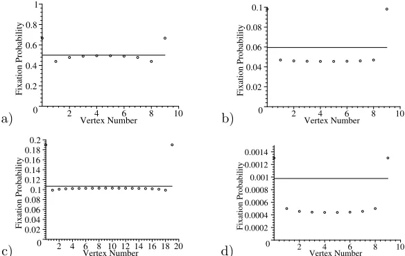
Figure 9. Fixation probabilities at vertices in a line withn+1 vertices. a)r= 2, n+1 = 10, b)r= 0.9, n+ 1 = 10 c)r= 1.1, n+ 1 = 20 , d)r= 0.5, n+ 1 = 10. The line corresponds to the level of the Moran process fixation probability.
Why is the mutant fitter on a line than a circle if and only if r > 1? The key reason for this is related to the behaviour at the end vertices. The fixation probabilities for a mutant placed into a specific vertex are given in figure 9. The end vertices 0 and nhave the highest fixation probability - because the only way the mutant can go extinct is by being replaced by a resident from vertex 1 orn−1, respectively. But even if a resident at 1 orn−1 is selected for reproduction, it has only a 50% chance (ifn+ 1>3) that it will place its offspring in the corner.
There is a steep drop in fixation probabilities for the vertex adjacent to the corner, 1 or n−1, since a mutant placed at 1 has a very high chance of being replaced by a resident from 0 (which, if selected has to place its offspring at 1).
[image:16.612.134.426.258.443.2]proba-a) 0
0.05 0.1 0.15 0.2
Fixation Probability
2 4 6 8 10
Vertex Number b) 0
0.1 0.2 0.3 0.4 0.5
Fixation Probability
2 4 6 8 10
[image:17.612.139.424.92.180.2]Vertex Number
Figure 10. Fixation probabilities at vertices in a line withn+ 1 vertices. Circles - single mutant present, diamonds - two mutants present in neighbouring vertices, boxes - three mutants present in neighbouring vertices. a)r= 0.9, n+ 1 = 10 , b) r= 1.1, n+ 1 = 10. The horizontal lines correspond to the level of the Moran process fixation probabilities when 1, 2 or 3 mutants are present in the population.
bility as given by the formula for the Moran process. Generally, the higherr, the shorter the line can be to have the central vertices equivalent to the corresponding Moran process. In other words, the higherr, the shorter is the range of the effect of the corner end point. Being near the centre can be thought of as equivalent to being in a circle; for an advantageous mutant once it has spread to be next to the corner (the first time it is influenced by the corner) it is likely that there will be many mutants and fixation will be almost assured. The most common way advantageous mutants are eliminated is early, due to bad luck, and so the corners do not affect the fixation probability of such mutants much (and hence why the larger r, the stronger this effect).
This is not true, however, for the caser <1. This is an interesting qualitative distinction betweenr < 1 and r >1, and occurs because non-advantageous mu-tants are unlikely to reach fixation unless by chance they reach a large proportion of the population, and so the corner will influence their fixation probability no mat-ter where they start. In fact securing a corner position seems important for their eventual survival, so being near a corner is better than being in the centre, even though this means that very early removal is more likely (the non-advantageous mutant needs to be lucky to reach fixation).
A similar pattern holds for larger groups of mutants on the line. Figure 10 shows the situation once a small group of mutants has been established, comparing the fixation probabilities for such a configuration of several mutants in their different possible positions.
8. Discussion
In this paper we have considered the use of evolutionary dynamics on graphs pop-ularised by Lieberman et al. (2005). We have found an analytic way, using the work of Miller (1994), to obtain the fixation probability of mutant populations for one particular type of graph, a line. We cannot find explicit functional forms, but rather a set of N simultaneous linear equations, whereN is the population size, which need to be solved and then yield the probability of fixation in any allowable situation. This is a significant saving on the order ofN2equations derived directly
by considering the transition probabilities between the states of our system. We have used our solutions to consider various examples and explore the rela-tionship between the fixation probability of a mutant on the circle, given by the Moran probability, and the fixation probability on the line; both the average such probability and its value for given starting positions. We see that for mutants that are fitter than the resident population the fixation probability on the line is larger than on the circle. There is also an interesting pattern in the fixation probability for the different starting positions on the line. The best place for a mutant to start is always in the corner. For advantageous mutants, the place next to the corner is the worst and fixation probabilities increase towards the central positions. For mutants that are not advantageous, the further from the corner they are, the worse the position they are in. It should be noted that the probability of fixation for non-advantageous mutants for graphs with more than a small number of vertices is generally low, so the results for advantageous mutations are the more interesting.
In §4 we show that for more complex graphs (which are the vast majority of graphs not of our linear type) almost all system states are reachable from almost all others, and so the number of equations generated by considering the transition probabilities is not of the orderN2 but much larger. For some graphs with a lot
of symmetry the number of equations can be reduced considerably, and in§5 we analyse one well known such case, the star, to produce an exact solution for the fixation probability of a mutant. However, graphs which can be solved in this way are special cases and the approaches that we take here for a line or a star will be hard to implement elsewhere. Thus it is likely that we will have to resort to more numerical methods, as in Rycht´aˇr & Stadler (2008); Santoset al. (2006); Paleyet al.(2007).
However, to gain an insight into deeper aspects of the problem and the effect of various structures, analysis is useful and in future work we intend to use approxi-mation methods to investigate this. This has the benefit of extending to larger more complex graphical systems, such as the small world networks of Bollobas & Chung (1988) (see also Durrett (2007), Newman et al. (2006), Newman & Watts (1999) and Watts & Strogatz (1998)). Small world graphs are regular in form with most vertices unconnected, but with a few added random connections which generally make the path length between any two vertices short.
References
Barabasi, A & Albert, R. 1999 Emergence of scaling in random networks.Science
286, 509–512.
Bollobas, B. & Chung, F.R.K. 1988 The diameter of a cycle plus random matching.
SIAM J. Discrete Math1, 328–333.
Bramson, M. & Griffeat, D. 1981 On the Williams-Bjerknes Tumour Growth Model
I.The Annals of Probab.9(2), 173–185.
Durrett, R. 2007Random Graph Dynamics, Cambridge University Press.
Erd¨os, P. & Renyi, A. 1960 On the evolution of random graphs.Publ. Math. Inst.
Hungarian Acad. Sci 5, 17–61.
Lieberman, E., Hauert, C., Nowak, M.A. 2005 Evolutionary Dynamics on Graphs.
Nature 433, 312–316.
Miller, J.W. 1994 A matrix equation approach to solving recurrence relations in two-dimensional random walks.J. Appl. Probab.31(3), 646–659.
Nagylaki, T. & Lucier, B. 1980 Numerical analysis of random drift in a cline.
Genetics 94, 497–517.
Newman, M.E.J., Barabasi, A.L., Watts, D.J. 2006The Structure and Dynamics
of Networks, Princeton Studies in Complexity, Princeton University Press.
Newman, M.E.J. & Watts, D.J. 1999 Renormalization group analysis of the small-world network modelPhys. Lett. A263, 341–346.
Norris, J.R. 1997.Markov Chains, Cambridge University Press.
Nowak, M.A. 2006Evolutionary Dynamics: exploring the equations of life, Harward University Press.
Paley, C.S., Tarashkin, S.N., Elliot, S.R. 2007 Temporal and dimensional Effects in Evolutionary Graph Theory.Physical Review Letters 98(9), 098103.
Rycht´aˇr, J. & Stadler, B. 2008 Evolutionary Dynamics on Small-World Networks.
Int. J. of Mathematics Sciences 2(1), 1–4.
Santos, P.C., Pacheco, J.M., Lenaerts, T. 2006 Evolutionary Dynamics of Social Dillemas in Structured Heteregenous Populations.PNAS 103(9), 3490–3494.
Tucker, A.C. 1994Applied combinatorics (3rd ed.), John Wiley & Sons, Inc.
Watts, D.J. & Strogatz, S.H. 1998 Collective dynamics of ‘small-world’ networks.