Numerical simulation of interaction between wind and 2D freak waves

City, University of London Institutional Repository

Citation:

This is the accepted version of the paper.

This version of the publication may differ from the final published

version.

Permanent repository link:

Link to published version:

Copyright and reuse: City Research Online aims to make research

outputs of City, University of London available to a wider audience.

Copyright and Moral Rights remain with the author(s) and/or copyright

holders. URLs from City Research Online may be freely distributed and

linked to.

City Research Online: http://openaccess.city.ac.uk/ [email protected]

Numerical Simulation of Interaction between Wind and 2-D Freak Waves

S. Yan and Q.W. Ma

School of Engineering and Mathematical Sciences, City University, London, EC1V 0HB, UK

Abstract

This paper presents a newly developed approach for the numerical modelling of wind effects on the

generation and dynamics of freak waves. In this approach, the quasi arbitrary Lagrangian-Eulerian finite

element method (QALE-FEM) developed by the authors of this paper is combined with a commercial

software (StarCD). The former is based on the fully nonlinear potential model, in which the wind-excited

pressure is modelled using a modified Jeffreys’ model (C. Kharif, et al. J. Fluid Mech. 594:209-247,2008).

The latter has a volume of fluid (VOF) solver which can handle violent air-wave interaction problems. The

combination can simulate the interaction between freak waves and winds with an improved computational

efficiency. The numerical approach is validated by comparing its predictions with experimental data.

Satisfactory agreements are achieved. Detailed numerical investigations of the interaction between winds

and 2D freak waves are carried out, which not only explore different air flow states but also reveal the wind

effects on the change of freak wave profiles. Both breaking and non-breaking freak waves are considered.

Key words: Freak waves; Wind effects; QALE-FEM; Numerical simulation

1. Introduction

Freak waves (also called rogue waves) have attracted a lot of attention from scientists and engineers. They

pose a real threat to human activities in the oceans despite their low possibility of occurrence [1]. A great

deal of efforts has been made to experimentally and numerically study the generation mechanisms and the

physical properties of freak waves (e.g. [2]-[3]). Detailed reviews may be found in [4]-[6]. However, most

of them are studied under ideal conditions, e.g. ignoring the wind effects. Although some freak waves have

been observed under good weather conditions with light winds, there are evidences that freak waves are

often accompanied by strong winds (e.g. [7]). These observations initiate two questions. The first one is

about whether the formation of freak waves is caused by the wind and the second one is about how the wind

first question have been found in literatures. The second one has been experimentally and numerically

studied by Giovanangeli et al. [8], Kharif et al. [9] and Touboul et al. [10], which mainly concluded that the

forwarding wind may shift the focusing point and increase the wave amplitude for 2D freak waves due to

spatio-temporal focusing. Although 2D cases are very rare in reality, investigations on 2D cases can shed

some light on main issues and the corresponding results may be useful reference for 3D studies. Therefore,

this paper still focuses on 2D studies about the second problem using numerical techniques. To do so, two

issues must be addressed.

The first one is the freak wave generation. Due to the complexity of the real sea condition which involves

winds, currents and waves, the physical mechanism of freak wave generation is still an open question.

However, based on previous research ([5],[11]), one of the possible mechanisms of freak wave generation

may be due to energy focusing, i.e. the wave energy concentrating in a small spatial area during a short time

and thus generating an abnormally large wave. There are many reasons for such an energy focusing, mainly

including spatio-temporal (dispersive) focusing (i.e. frequency and/or directional focusing) of transient wave

groups (e.g. [12]-[16]), wave-current interaction [17], geometrical focusing due to seabed topography [18]

and nonlinear modulation instability [9,19]. For 2-D simulations, the freak waves are usually generated

using a wavemaker whose motion is mainly specified by one of the following ways: (1) using a sine function

with linearly variable frequency with the largest frequency at the start (e.g. [9-10]); (2) using the sum of a

number of sine or cosine wave components with different frequencies (e.g. [2],[4] and [20]); (3) using

signals composed of normal random waves and a freak wave [21]; and (4) using the signals obtained by

performing Fourier analysis of the observed time history of sea states containing freak waves[22].

The second issue is the coupling effect between freak waves and winds. In one aspect, wind may

dramatically influence the shape of wave profiles. This has been shown by laboratory observations with the

fact that forwarding wind may move the breaking point further downstream [23-25] and an opposing wind

may result in wave attenuation for harmonic waves [26]. In the other aspect, the propagation of the waves,

in turn, affects the property of the air flow and may cause air-flow separation and/or vortex shedding, which

ultimately alter the free surface pressure and thus wave propagation. These effects have been confirmed

also by physical experiments for breaking waves, which demonstrated that the waves may result in different

wind-excited free surface pressure distributions [27], the occurrence of air flow separation [28] and the

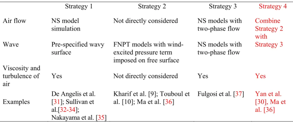
Due to its complexity, various numerical strategies have been developed. They may be classified into four

categories as summarised in our previous publication [30]. Nevertheless, sufficient details will be described

here for completeness. Table 1 lists four strategies. Considering the strong nonlinearity associated with

freak waves, fully nonlinear models, i.e. either the fully nonlinear potential (FNPT) model or the general

Navier-Stokes (NS) model, are necessary for such problems [4,6]. Therefore, only studies related to fully

nonlinear models are cited in this table.

Table 1. Summary of numerical strategies addressing strong interaction between winds and waves

Strategy 1 Strategy 2 Strategy 3 Strategy 4

Air flow NS model

simulation

Not directly considered NS models with two-phase flow

Combine Strategy 2 with Strategy 3

Wave Pre-specified wavy

surface

FNPT models with wind-excited pressure term imposed on free surface

NS models with two-phase flow

Viscosity and turbulence of air

Yes Not directly considered Yes Yes

Examples

De Angelis et al. [31]; Sullivan et al.[32-34];

Nakayama et al. [35]

Kharif et al. [9]; Touboul et al. [10]; Ma et al. [36]

Fulgosi et al. [37] Yan et al. [30], Ma et al. [36]

In the first category, the profile of the water free surface is pre-specified. The waves are therefore

considered to be wavy surfaces (either rigid or flexible) moving with a specific speed (usually wave celerity).

Only the air flow over the wavy surface is simulated. Therefore, it is relatively simple and can give some

interesting insights on the second aspect of the wind-wave interaction, e.g. the wind-excited free surface

pressure/stress feature or the turbulent structure of the air flow [31-35], but it cannot study the second aspect

of the wind-wave interaction, i.e. the effects on the changes of the wave shape.

The second strategy is to numerically simulate the water waves without directly considering the air flow.

The wind effects are modelled by introducing an extra free surface pressure term or energy

source/dissipation terms in the free surface boundary condition. The extra pressure/energy terms are based on

wave-air interaction mechanisms, such as Jeffreys’ sheltering mechanism [38-39], Miles’ shearing

mechanism [40-42] and other mechanisms quantifying the consequential growth rate of the waves, e.g.

developed a boundary integral equation method (BIEM) to simulate wind effects on 2D freak waves. In their

model, the wind effects are modelled by using the modified Jeffreys’ sheltering mechanism. However, a

limitation in these numerical models is that the dynamics of viscosity and turbulence of air could not be fully

taken into account. Apart from this, the strategy could not take into account the effects of the waves on the

air flow.

In the studies adopting the third strategy, the Navier-Stokes (NS) equations for two-phase flow are solved.

In other words, the air flow and the waves are solved simultaneously. Therefore, the aspect of mutual

interaction between winds and waves can be fully considered. Many methods, such as finite volume method

(e.g. [45-49]), finite difference method (e.g. [50]) and CIP (Cubic interpolated propagation) method [51]

have been developed for solving the NS equations. However, they have rarely been applied to interaction

between winds and freak waves or breaking waves, though they all have the potential to do so. That is

partially because of the high computational cost. Only one paper [37] was found to simulate interaction

between wind and non-breaking waves using a two-phase model.

In addition, one may combine the NS two-phase flow model with a FNPT model adopting the second

strategy, regarded as the fourth strategy. That is, the third strategy in the area with strong interaction

between winds and freak waves is applied but the second strategy is employed otherwise. It would be

understandable that the fourth strategy may be able achieve similar accuracy as the third strategy but require

much less computational costs. Similar idea has been adopted by Lachaume et al. [52] and Garzon et al. [53]

to simulate 2D breaking waves. However, the wind effects were not taken into account in their studies.

Ma and Yan [36] have investigated the fourth strategy and carried out preliminary studies on the wind

effects on freak waves. In their approach, an in-house software package (QALE-FEM/FLOATMov) is

combined with a commercial software, StarCD. The former is based on the FNPT model, which has been

proven to be the fastest method for overturning waves [54, 55]. The latter solves general

Reynolds-Averaged Navier-Stokes (RANS) equations using the finite volume method. The free surface is tracked by

the Volume of Fluid (VOF) method. Also by using this approach, Yan and Ma [30] investigated the wind

effects on the breaking solitary waves and explored the air flow separation and vortex shedding involved.

For brief, this approach is referred to as QALE-FEM/StarCD in the rest of this paper. This paper will further

investigate the interaction between winds and 2D freaking waves, which are generated in the first or second

flow and wind effects on the change of freak wave profiles will be discussed. The wind-excited pressure on

the free surface will be analysed. For some cases, the results are compared with the experimental data and

satisfactory agreements will be presented.

2. Mathematical model and numerical approach

As mentioned above, the approach adopted here is to combine the QALE-FEM with the StarCD. All

numerical investigations are carried out in a numerical tank with a flat seabed and a mean water depth of d.

A wavemaker is mounted at the left side of the domain. The Cartesian coordinate system is adopted with the

x-axis on the mean free surface and the z-axis being positive upwards. The origin of the coordinate system

is located at the initial position of the wavemaker. Before the combination of these two methods is discussed,

necessary summaries of them are first presented.

2.1. QALE-FEM formulations and Jeffreys’ theory

In the QALE-FEM method, only the water is considered and the air above the free surface is not included

in the calculation. The motion of the water wave is governed by Laplace’s equation about the velocity

potential () together with fully nonlinear boundary conditions imposed on the free surface and moving

rigid boundaries. The details of the QALE-FEM can be found in our previous publications ([4],[54-55]) for

the cases without wind.

In order to consider the wind effects, the dynamic condition on the free surface z







by introducing an extra term representing the wind-excited pressure. This condition is written in the

following Lagrangian form,

sf p gz

Dt

D _{  } 2_ 2

1 _



, (1)

in which

D/Dt

g

acceleration and psf the free-surface pressure, which is taken as zero for the cases without wind (e.g. [4],[

54-57]). For those with wind, the Jeffreys’ sheltering mechanism used by Kharif et al. [9] and Touboul et al. [10]

is applied to evaluate psfas follows,

x c U s

psf a w g _

 

 _{( )}2  _{, (2)}

where the constant s is the sheltering coefficient and is taken as 0.5 according to our numerical investigation.

a

the speed of the wave motion. Kharif et al. [9] assigned the wave phase velocity to cg. This is reasonable

for harmonic waves. In this paper, the characteristic velocity of the wave motion is chosen as the group

velocity (Ug) rather than the phase velocity, because it is more reasonable for freak waves or wave groups.

2.2. StarCD formulations and the implementation of boundary conditions

The commercial software StarCD solves the Eulerian RANS equations and the continuity equation. The

free surface is tracked by using the VOF method. For this purpose, a fraction function C is defined. It is 0

for the air and 1 for the water. A transport equation of C is solved together with other governing equations.

To consider the turbulence, the k-ε/High Reynolds Number turbulence model is chosen. The details of the

StarCD on solving free surface problems can be found in the StarCD user guide [58]. However, some

pertinent details on implementation of boundary conditions will be described here for the problems

considered in the paper.

On the inlet boundary, the following Dirichlet conditions are specified,

v

f

v

,

(3)

where v is the fluid velocity; fv and fCI denote the fluid velocity and the value of the fraction function C,

respectively, on the inlet boundary at every time step. On the outlet boundary, the following pressure

boundary condition is imposed,

p f

p

,

(4)

in which fp and fCp represent the pressure and the fraction function C on the outlet boundary, respectively.

Apart from these, a non-slip wall condition is specified on the seabed. The top wall in this case may not

exist in reality. Unless mentioned otherwise, the top wall is considered as an artificial wall and assigned to

be parallel to the incoming wind velocity (it is horizontal in all cases presented in this paper) with a slip wall

condition being imposed. It should be noted that on such an artificial wall, one may also use the non-slip

wall condition. However, a higher tank than the corresponding case with the slip wall condition is required in

order to eliminate the wall effects according to our numerical test. A zero-gradient turbulence condition is

employed on inlet and outlet boundaries of the domain.

2.3. Combination of QALE-FEM and StarCD

For time-domain simulations, one may use two ways to combine the QALE-FEM and the StarCD. In the

and the latter being applied in the second period. This combination may be justified that in the first period of

the time domain, the waves are relatively small and the QALE-FEM with a modified Jeffreys’ theory may be

sufficiently accurate. Alternatively, one may also decompose the whole spatial domain into several

sub-domains and different methods are employed in different sub-sub-domains. In the QALE-FEM/StarCD

approach, the second way is implemented. The whole spatial computational domain is decomposed into two

sub-domains, as shown in Fig. 1. The first one (ΩF) ranges from the wavemaker to an artificial boundary

with a length of LF and the second one (ΩS) covers the rest part of the domain. The QALE-FEM model and

the StarCD are adopted in ΩF and ΩS, respectively.

Fig. 1. Sketch of computational domains for QALE-FEM/StarCD approach (Dashed rectangle: QALE-FEM sub-domain; Solid rectangle: StarCD sub-domain)

One may run the QALE-FEM model and the StarCD simultaneously at every time step and use an

iteration procedure to couple the condition on the boundary (ΓI) between two sub-domains. However, it is

difficult to implement in the StarCD. Further, the iteration procedure dramatically increases the CPU time.

To avoid the iteration procedure, in the current QALE-FEM/StarCD approach, the QALE-FEM calculation

in ΩF and the StarCD calculation in ΩS are carried out separately. The whole procedure is therefore separated

into two stages. At each stage the calculation starts from t = 0 and stops when the required duration of

simulation is achieved.

In the first stage, the QALE-FEM calculation is run. A relatively larger fluid domain than the sub-domain

ΩF is adopted. In order to absorb the reflection, a damping zone with length of Ld= min(3d, 3max) is

applied at the right side of the sub-domain with max being the longest wavelength of all wave components

and a Sommerfeld condition is imposed at the truncated wall of the fluid domain[59]. According to our

numerical test, the length of the sub-domain used in this stage of calculation is taken as LF+3d+ Ld. The

velocity and the wave elevation (_i) at x=LF (corresponding to the position of the boundary ΓI of ΩS in Fig.

Wind

Free surface

ΓI

ΓP

Wave maker

ΩF 20 ΩS: RANS + Continuous Eq.

z

x

ΓB

1) are recorded at every time step for the purpose of providing the boundary condition for the StarCD

simulation in the second stage.

In the second stage, the StarCD calculation is run in the sub-domain ΩS sketched in Fig. 1. On its inlet

boundary (ΓI), fCI in Eq. (3) is specified by using the wave elevation (i) at this position calculated by the

QALE-FEM. In this work, rectangle cells are used by the StarCD. For each cell, fCI is specified as follows,

            i i i i CI z z z z z z z f









in which zmin and zmax are the minimum and maximum values of z-coordinates of 4 vertexes of a cell,

respectively. The fluid velocity fv in Eq. (3) is given by

          1 1 0 0 C u C u C U f z sf w v    (5b)

where Uw (Uw,0)



; u_sf is the fluid velocity on the free surface recorded at x=LF; uz is the fluid velocity at

corresponding position from the seabed to the free surface at x=LF. Both usf and uz are calculated using

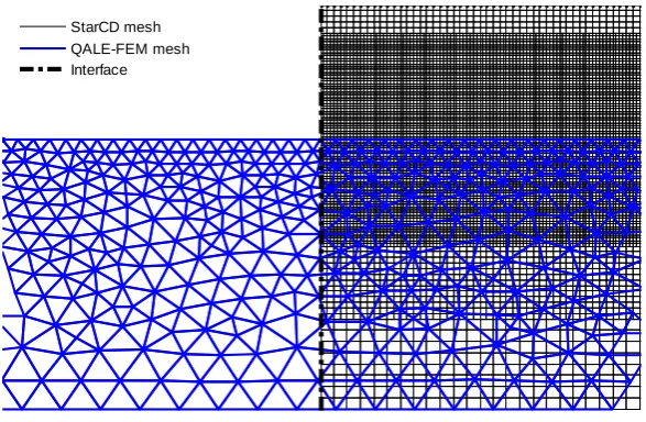
the QALE-FEM at the first stage. Because the mesh used in the QALE-FEM is different from that in the

StarCD (Fig. 2), the nodes in the latter are not coincident with those in the former on the boundary (ΓI).

Therefore, a moving least square method is employed in the space domain to find the velocity and wave

elevation at the inlet boundary (ΓI) for the StarCD calculation using the data recorded in the first stage.

StarCD mesh QALE-FEM mesh Interface

Apart from this, one may use different time step for the QALE-FEM and StarCD calculations. According

to our numerical test, the time step required by the StarCD is much smaller than (roughly 1/10 of) that

required by the QALE-FEM to achieve convergent results. To obtain the information at smaller time steps

for the StarCD, a second order polynomial interpolation scheme is applied in the time domain to find the fCI

and fv at specific instants.

It should be pointed out that the reflections from the downstream truncated boundaries of the StarCD

sub-domain are undesired. In order to absorb the reflection, one may develop a damping technique by

introducing an extra energy sink term in the StarCD simulation or adopt another QALE-FEM sub-domain to

the right side of the StarCD sub-domain (ΩS) because the QALE-FEM has a capacity to suppress the

reflection. Nevertheless, a sufficient long tank is applied in this paper to eliminate the reflection, rather than

making much effort on the absorbing techniques. By using this technique, fpin Eq.(4) can be taken as the

static pressure. This condition is acceptable before the incoming wave reaches the truncated boundary.

2.4. More discussion on the QALE-FEM/StarCD approach

As indicated above, the StarCD has been developed to solve general RANS equations by using the finite

volume method with the VOF method adopted to track the free surface. It can model the coupling between

the water waves and air flows. It can also take into account of the turbulent effects. However, it is very

time-consuming compared with the QALE-FEM. There are two main reasons for why the computational

cost of the StarCD is much higher than the QALE-FEM. The first one is that the number of unknowns in the

governing equations adopted by the former is much larger than that in the latter. The second one is that it

needs much smaller element size and much shorter time step to reduce the numerical diffusion. Apart from

the computational efficiency, another difficulty associated with the StarCD is the wave generation. In the

experiments and nonlinear numerical investigations, performed earlier, freak waves are usually generated

using a wavemaker. The motion of the wavemaker causes the change of fluid domain during the calculations.

But, the StarCD solves Eulerian model and the fluid domain is required to be fixed during the calculation.

Therefore, the technique of the wavemaker cannot be easily applied unless other techniques are employed.

Alternatively, one may specify velocities and the wave elevations at the inlet boundary of the computational

domain prior to solving the governing equations of the StarCD. However, those parameters are usually

The QALE-FEM is based on the fully nonlinear potential theory, which has been proved to be the fastest

method for modelling nonlinear overturning waves ([6], [54-57]). Our numerical investigation on 2D freak

waves has also revealed that it needs only 1/30 to 1/10 of the CPU time required by the StarCD to achieve

the results with the same accuracy level. In addition, the QALE-FEM allows the fluid domain to be

deformed following the motion of the wavemaker. By specifying the motion of the wavemaker, it can

generate nonlinear waves in a way similar to the physical experiments. In our previous publications, the

QALE-FEM has been successfully applied to simulate 2D and 3D freak waves [4, 6]. The wind effects in

this method are modelled by introducing an extra term representing the wind-excited pressure on the free

surface based on the Jeffreys’ theory. However, the viscous and the turbulent effects can not be considered

in this method.

The approach QALE-FEM/StarCD combining the two codes together not only solves the problems

associated with the StarCD and the QALE_FEM but also allows the StarCD to be used only within the areas

where strong interaction between freak waves and winds may occur, thus reducing the computational domain

of the StarCD and saving computational time. Nevertheless, special care must be taken about how to choose

the interface between them. The required quantitative information is currently not available about determining

the position of the boundary ΓI (or the length LF of the sub-domain ΩF ). A related investigation is carried out

in this paper.

3. Numerical results and discussions

In this section, the wind effects on the change of the freak wave profiles and related physical properties,

such as free surface pressure and vorticity distribution, are investigated. For convenience, the parameters

with a length scale are nondimensionalised by the water depth d, the time t by d/g ( i.e. t/ d/g ), the

velocity/speed by gd , where τ is the nondimensionalised form of the time. The vorticity and pressure are

nondimensionlised by |Uw-Ug|/At and ρa(Uw-Ug)2, respectively, in which Atis the targeted wave height.

3.1 Comparison with experimental data

The QALE-FEM/StarCD approach is first validated by comparing its numerical results with the

experimental data in Kharif et al. [9] and Touboul et al. [10]. The case considered here is about a 2D breaking

respectively. The freak wave is generated by a wavemaker that undergoes a motion defined by a sine

function. The frequency in the sine function varies linearly from the maximum frequency (ωmax) to the

minimum frequency (ωmin) in a duration of 31.32 with ωmin =1.6 and ωmax = 2.6. The theoretical focusing

point is 17 away from the wavemaker and focusing time is about 81.4. The wind with the speed Uwof 1.916

in the same direction of the freak wave propagation blows above the free surface. In the numerical

simulation, the sub-domain for the StarCD starts at x=1, i.e. LF = 1. The mesh size near the free surfaces and

the time step for the QALE-FEM are chosen as 0.05 and 0.025, according to convergence investigations [55].

To investigate the convergence property of the StarCD in this case, different mesh sizes, ranging from 0.003

to 0.006 are chosen. The time step required by the StarCD is dependent on the mesh size and fluid speed.

The maximum Courant number is configured to be 0.3 as suggested by [58]. Although the time step (dτ) is

taken as 0.003 for all the mesh sizes used here for this wind speed based on our numerical tests, the StarCD

may automatically reduce the step size and carry out sub-step calculation, depending on whether the Courant

number is larger than the configured maximum value, i.e. 0.3. To be consistent with the experimental

configuration, a non-slip condition is imposed on the top wall in this case.

The piston-type wavemaker is used in the numerical simulation. In the duration of Tfh, the motion of the

wavemaker is governed by

]

)

(

cos[

)

(

0













d

F

a

S

when τ≤Tfh ; otherwise S(τ)=0. In Eq.(6), a is the expected wave amplitude, which is given as 0.03, and F is

transfer function of the wavemaker [4] which is given by

k

k

k

F

2

)

2

sinh(

]

1

)

2

[cosh(

2







wherek is the wave number corresponding to frequency ω(τ). They are related to each other by ω2=ktanh(k)

and ω(τ) linearly decreases from ωmax to ωmin in the duration Tfh. Because the wavemaker used here is

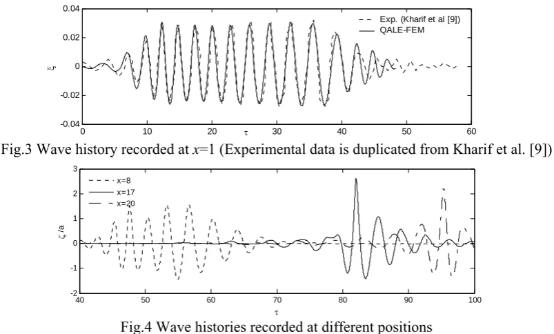
different from that in the experiment. To make sure that the generated waves are consistent, the wave history

recorded at x=1 (at the inlet boundary of the StarCD domain) is compared with the experimental data

0 10 20 30 40 50 60 -0.04

-0.02 0 0.02 0.04





Exp. (Kharif et al [9]) QALE-FEM

Fig.3 Wave history recorded at x=1 (Experimental data is duplicated from Kharif et al. [9])

40 50 60 70 80 90 100

-2 -1 0 1 2 3





/a

x=8 x=17 x=20

Fig.4 Wave histories recorded at different positions

(StarCD cell sizes: 0.003; free surface elevation obtained using the VOF fraction = 0.5)

Fig.4 displays wave histories recorded at different positions. In this case, the StarCD cell size is taken as

0.003 and the free surface is identified using the VOF fraction equal 0.5. From this figure, it is found that at

the theoretical focusing point (x ≈ 17), the free surface elevation reaches its maximum value at τ≈ 81.4, the

theoretical focusing time, which is consistent with the result from Kharif et al.[9] and Touboul et al [10] . It

is also observed that the wave elevation varies at different positions. To examine how the wave elevation

changes along the direction of the wave propagation, an amplification factor A, which was defined by Kharif

et al [9], is used,

ref H H

A max/ , (8)

in which Hmax is the maximum wave height between two consecutive crest and trough of a wave history

recorded at different position throughout the tank; Href = 0.0613 is the average wave height of the wave train

at the inlet of the tank (measured at x=1) between τ≈12 and τ≈37. The computed amplification factor A as a

function of distance from the left side of the tank is compared with the experimental results in Fig.5.

6 8 10 12 14 16 18 20 22

1 1.5 2 2.5

A

x ds=0.003

ds=0.004 ds=0.005 ds=0.006 Exp. (Kharif et al.[9])

Fig.5 Evolution of the amplification factor A as a function of distance (wind speed Uw=1.916, Href=0.0613) in

It is observed from Fig.5 that the numerical results seem to be very sensitive to the mesh size. The

numerical results become closer to the experimental data as the mesh size (ds) decreases. Considering the

complexity of the air-wave interaction involved in this case the agreement between the results of ds =0.003

and the experimental data can be considered as acceptable. One may also find that for the cases with

004 . 0 

ds , the differences between the numerical results and the experimental data are small when x<6,

but they become larger as x further increases. This suggests that such differences may be caused by the

numerical diffusion. The investigation implies that by assigning proper cell size, the current

QALE-FEM/StarCD approach can lead to sufficiently accurate results. Similar to all other numerical methods, the

convergence property of this approach may be problem-dependent and need to be investigated with care.

3.2 Wind effects on 2D freak waves

The QALE-FEM/StarCD approach is now applied to study the interaction between winds and 2D freak

waves. For this purpose, the freak waves are generated using a sum of a number of sine (cosine) wave

components. The displacement of the wavemaker (e.g. [2] and [4]) is given by





  N

n n n n

n F a S

1

) cos(

)

(    , (9)

where N is the total number of components and Fn is the transfer function of the wavemaker which can be

calculated using Eq.(7). kn and ωn are the wave number and frequency of the n-th component, respectively.

The frequency of the wave components are equally spaced over the range [ωmin, ωmax]. εn is the phase of the

n-th component and is chosen to be knxf - ωn τf with xf and τf being the expected focusing point and the

focusing time according to linear theory [2,4]. an is the amplitude of n-th component, which is taken as the

same for all components in this paper to simplify the relationship between the target amplitude (At) of the

freak wave and the amplitudes of the components, leading to an=At /N.

In the case considered below, ωmin = 0.5 , ωmax = 1.4, N=32, an =0.008 (At =0.256). The linear group

velocity (Ug) is 0.5972. xf and τf are assigned to be 10 and 31.32, respectively. Different wind speeds,

ranging from 0 to 3.832, are chosen. The length of the tank L is taken as 40, equal LF+LS. According to the

numerical test, the height of the StarCD sub-domain is taken as 10 to eliminate the effects of the top wall.

As indicated above, there is an interface between the sub-domains in this approach, on which interpolation

in space and time domains is required. One may ask whether it would produce unacceptable error and where

it should be or how to choose LF, which determining the location of the artificial boundary between the

QALE-FEM sub-domain and the StarCD sub-domain. To answer these questions, the effect of LF on the

wind-wave interaction is first investigated. The wind speed in this investigation is assigned to be 3.832

(equivalent to 12m/s in case with water depth of 1m), the largest value used in the paper. The value of LF

varies from 1 to 7, i.e. from 2.5% to 17.5% of the tank length L. According to the convergence investigation,

the mesh size and time step for the QALE-FEM are 0.05 and 0.025, respectively. Those for the StarCD

calculation are 0.009 and 0.0015, respectively. The maximum Courant number is configured to be 0.3. The

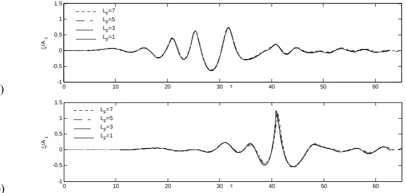
wave profiles near the wavemaker at different instants in the cases with different values of LF are plotted in

Fig. 6.

1 2 3 4 5 6 7 8 9 10

-1 -0.5 0 0.5 1 1.5 x  /A t L F=1 L F=3 L F=5 L F=7

1 2 3 4 5 6 7 8 9 10

-1 -0.5 0 0.5 1 1.5 x  /A t L F=1 L F=3 L F=5 L F=7

(a) τ≈16.4 (b)τ≈21.1

Fig.6 Wave profiles near the wavemaker in the cases with different LF (Uw=3.832, ωmin=0.5, ωmax=1.4, xf =10,

τf =31.32, N=32, an=0.008)

(a)

-0.5 0 0.5 1 1.5   /A t

L_F=7 L_F=5 L_F=3 L_F=1

(b)

-0.5 0 0.5 1 1.5   /A t

L_F=7 L_F=5 L_F=3 L_F=1

Fig.7 Wave histories recorded at (a) x=7 and (b) x=15 in case with different LF (Uw=3.832, ωmin=0.5,

One may find from Fig. 6 that near the inlet boundaries of the StarCD sub-domain (x=LF), the free surface

profiles are smooth no matter which LF is chosen. It is also observed that the differences between the curves

for different LF are hardly distinguished, especially in the area x<3. This means that the results are not

sensitive to the position of the interface and the interpolation schemes in space and time domains required on

the interface work well. The comparison of wave histories recorded at different positions is also made to

shed light on the effect of LF in a long-time simulation. Some results are shown in Fig. 7. Fig. 7a displays

the wave histories recorded at a point close to the wavemaker (x=7) in the cases with different LF and Fig.

7b shows the corresponding results recorded near the calculated focusing point (where the highest crest

occurs). As can be seen, the wave histories of LF =1 (2.5% L) and that of LF =3 (7.5% L) are still almost the

same, but the difference of the wave history between LF =1 and LF =7 (17.5% L) are visible, even though it

may still be acceptable. Based on these investigations, LF =3 is chosen in this paper.

As indicated above, in order to reduce the numerical diffusion existing in the StarCD simulation, one

needs to use a proper mesh size. Though a preliminary convergence investigation has been shown in Section

3.1, the convergence property is problem-dependent. To show our confidence in the results of the case

shown in Figs. 6 and 7, which will also discussed in the following two subsections, the related convergence

investigation is discussed here. Because the StarCD can automatically reduce the time step size once the

Courant number in the calculation exceeds the specified maximum Courant number, which is 0.3 in the

investigation. Therefore, the only factor which may affect the convergence property is the mesh size. Thus,

different mesh sizes, ranging from 0.008 to 0.012, are applied.

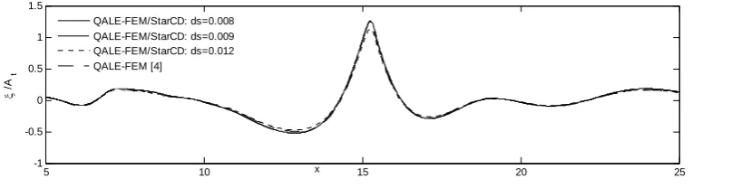
5 10 15 20 25

-1 -0.5 0 0.5 1 1.5



/A

t

x QALE-FEM/StarCD: ds=0.008

QALE-FEM/StarCD: ds=0.009 QALE-FEM/StarCD: ds=0.012 QALE-FEM [4]

Fig.8 Free surface profiles recorded at at τ≈ 41.49 in the case with different mesh sizes (Uw=0, ωmin=0.5,

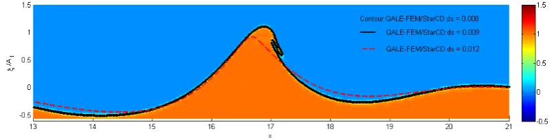
Fig. 9 Free surface profiles recorded at τ≈ 43.84 in the cases with different mesh sizes (Uw=3.832, ωmin=0.5,

ωmax=1.4, xf =10, τf =31.32, N=32, an=0.008)

For this case, the related experimental data is not available in the public domain. However, one may use

the QALE-FEM method, which has been validated by Ma [4], to produce the results without considering

wind effects, i.e. the case with Uw=0, for comparison. dτ in the StarCD configuration is initially given as

0.006. Fig.8 shows the comparison of free surface profiles recorded at τ≈ 41.49, when the wave focusing

occurs, in the case with Uw=0. It is found that when the mesh size is smaller than 0.009, the results from the

QALE-FEM/StarCD approach are almost the same and they agree well with the results in the case where

only the QALE-FEM is applied [4]; however, when the mesh size is larger, i.e. 0.012, the result is different

from the others.

Investigation is also made for the case with Uw=3.832, the largest wind speed applied in this paper. dτ for

the StarCD calculation is initially configured as 0.003 for all mesh sizes. In this case, a wave breaking occurs

due to the wind effects. The free surface profiles at one typical instant with a breaking wave are shown in

Fig.9, in which a contour of the VOF fraction function is given for the case with ds=0.008. Again, one may

also observe that the results with ds=0.008 and ds=0.009 are very close, though an acceptable difference with

relatively error less than 0.1% is found, which mainly exists near the tip of the overturning jet. However,

when the mesh size increases to be 0.012, the result is significantly different from others; most importantly,

the breaking is not observed in the case with such a mesh size. This investigation clearly demonstrates that

when ds≤ 0.009, the results are convergent. Based on this, ds is chosen to be 0.009 for the cases shown in

the following subsection.

3.2.2 Vortex shedding and air-flow separation

In the laboratory observation [29], the vortex shedding and air-flow separation were described. So far,

related numerical investigations of these phenomena in the cases with freak waves have not been found. To

illustrated in Figs. 10-13, which also include the computational parameters that are the same as those in Fig.

6 and Fig.7 except for the wind speeds and the time step. The time step here is larger (dτ=0.006 for StarCD

calculation) because the wind speed is smaller. The simulation was run on a PC with Intel 1.86GHz

processor (single CPU) and 2G RAM. The total CPU time to achieve results up to τ≈ 71 was about 132h.

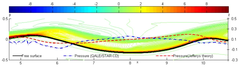
Fig. 10 displays the free surface profile, velocity/vorticity distribution and free surface pressures near a

wave crest at early stage of the wave propagation, when a relative large crest with the elevation of 0.16 just

appears. In the top part of Fig. 10a and Fig. 10b, the contour represents the vorticity in air whose value is

given by the colour bar above the plot. The solid and dotted lines denote the free surface profile and free

surface pressure recorded in the QALE-FEM/StarCD simulation, respectively. The dashed line is the

pressure calculated using Eq. (2) based on the original Jeffreys’ theory without considering the threshold

value of the free surface slope. As can be seen either from the contour of the vorticity (top part) or from the

velocity distribution (bottom part) of Fig. 10a, a large scale vortex occurs at the lee side of the crest (x≈ 6.5).

The distance between the wave crest and the centre of the vortex is about lcv ≈ 0.95 at τ≈ 23.49. It moves

further away from the crest following the motion of air flow and the propagation of the wave group in Fig.

10b (x≈ 7.2) with lcv≈ 1.15 at τ≈ 24.27.

Another vortex is shed following the occurrence of a secondly higher crest at the time τ≈ 29.75 as shown

in Fig. 11 where the crest with a height of 0.17 appears near x = 5.3. In this figure, the velocity distribution

is not shown to save the space. The further development of this vortex leads to the boundary layer separation

at the lee side of the crest as shown in Fig.12, where the wave crest height is about At and located near the

expected focusing point (xf). In the separation area, the vorticity and velocity of the air is very small. It is

evidenced by this investigation that the air flow structure above the free surface strongly depends on the

(a)

(b)

Fig. 10 Free surface profile, velocity/vorticity field and pressure distribution on the free surface near the wave crest at (a) τ ≈ 23.49 and (b) τ ≈ 24.27 (Uw=1.916, ωmin=0.5, ωmax=1.4, xf =10, τf =31.32, N=32,

an=0.008 , L=40, LF=3; QALE-FEM: ds=0.05, dτ=0.025; StarCD: ds=0.009, dτ=0.006)

Fig. 11 Free surface profile, vorticity field and pressure distribution on the free surface near the wave crest at τ ≈ 29.75 (Uw=1.916, ωmin=0.5, ωmax=1.4, xf =10, τf =31.32, N=32, an=0.008 , L=40, LF=3; QALE-FEM:

Fig. 12 Free surface profile, vorticity field and pressure distribution on the free surface near the wave crest at τ ≈ 35.23 (Uw=1.916, ωmin=0.5, ωmax=1.4, xf =10, τf =31.32, N=32, an=0.008 , L=40, LF=3; QALE-FEM:

ds=0.05, dτ=0.025; StarCD: ds=0.009, dτ=0.006)

3.2.3 Wind-excited free surface pressure

Apart from the vortex shedding and the air flow separation, the pressure distribution on the free surface is

also worthy of discussion. From Figs. 10-12, one may find that the free surface pressure features different at

different time. More specific details and comparison with the results from the Jeffreys’ theory are discussed

here.

From the Fig. 10 and Fig. 11 where vortex shedding just appears after the first crest, it is observed that the

free surface pressure is dramatically affected by the vortex (see x≈ 6.5 in Fig.10a and x≈ 7.2 in Fig. 10b).

As can be seen, a significant low trough of the free surface pressure appears under the centre of the vortex.

The magnitude of the trough seems to decrease with the decrease of the vorticity. On the other hand, the

corresponding results estimated by the Jeffreys’ theory do not show such behaviour. Apart from this,

another significant difference between the computed results and those from the Jeffreys’ theory exists in the

area near the wave trough after the first crest shown in Fig. 10 and Fig. 11. A larger pressure peak is

observed near the position where the wave trough occurs in the QALE-FEM/StarCD simulation. However,

the corresponding pressure from the Jeffreys’ theory is close to zero because the free surface slope at this

position is close to zero.

In contrast, at the instant shown in Fig. 12 where the air-flow fully separated, the free surface pressure

seems to be dominated by the free surface slope and the results by Jeffreys’ theory are close to the present

numerical results. This is due to the fact that the Jeffreys’ theory is based on the assumption that the

boundary layer is fully separated. However, this agreement sustains only a short time, because the wave and

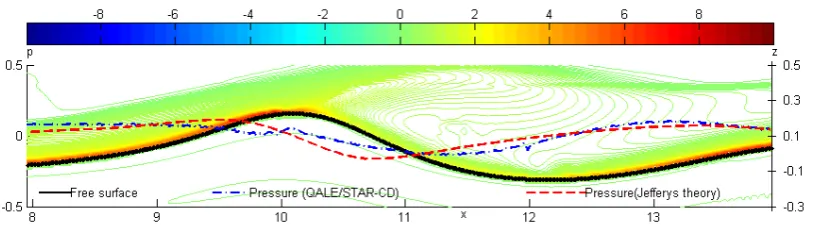
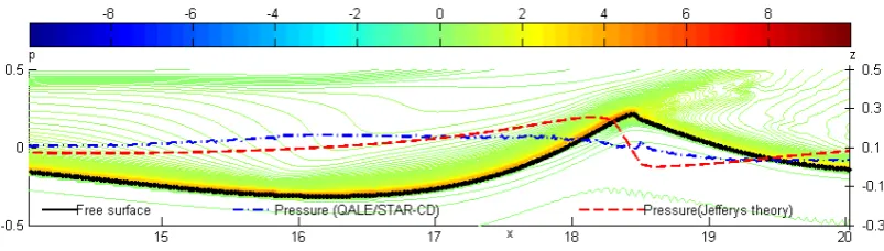
Fig. 13 Free surface profile, vorticity field and pressure distribution on the free surface near the wave crest at τ≈ 45.40 (Uw=1.916, ωmin=0.5, ωmax=1.4, xf =10, τf =31.32, N=32, an=0.008 )

Fig. 13 show the significant difference between the pressures recorded in the present calculation and those by

the Jeffreys’ theory, where the freak wave becomes very steep and tends to overturn. The latter is much

larger than the former near the wave crest. Apart from this, in the area to the left of the wave crest, the

pressure increases as the wave elevation decreases and the highest pressure is observed near the trough

where the free surface slope is close to zero. Similar to those in Figs. 10 and 11, the Jeffreys’ theory fails to

predict such pressure changing trend in this area.

As discussed above, the features of the pressure distribution are different with the propagation of the

freak wave. Typical features of the free surface pressure in this case are: (1) the pressure value may strongly

depend on the shedding vortex; (2) at some time step, a pressure peak may be observed near the trough

where the free surface slope is close to zero; (3) at the moments when the air flow is fully separated, the free

surface slope dominates the pressure distribution in the area near the wave crest. Although an acceptable

agreement between the wind-excited free surface pressure estimated by the Jeffreys’ theory and that by the

QALE-FEM/StarCD approach is observed at some time steps with fully separated air flow (similar to Fig.12),

the Jeffreys’ theory fails to provide acceptable results for pressure at many instants during propagation of the

freak wave, especially when vortex shedding or wave overturning occurs. Due to this fact, Kharif et al. [9]

and Touboul et al. [10] modified the original Jeffreys’ theory by introducing a slope threshold value for Eq.

(2), where the slope is estimated based on the free surface profile (solid line). In their modified Jeffreys’

theory, when the maximum free surface slope is larger than the threshold value, the free surface pressure is

taken as zero. As a possible way modelling wind effects, their work explained some actual phenomena as

discussed in the Introduction. For the cases without wave breaking, the amplification factor predicted using

theory and the numerical results at many instants may lead to some questions. For example, is the modified

Jeffreys’ theory still suitable beyond the cases considered? Are there any other models which can lead to

better approximation of the free surface pressure distribution and thus provide more accurate prediction than

the modified Jeffreys’ theory? These questions are not discussed here in detail but left to be addressed in our

future papers based on further investigations.

3.2.4 Wind effects on wave elevation/profile

In this sub-section, the wind effects on the change of the wave profile are investigated. Kharif et al. [9] and

Touboul et al. [10] carried out a similar numerical investigation using the FNPT based numerical model but

gave results for non-breaking waves. In reality, freak waves are likely to become breaking, particularly

under strong winds. Both breaking and non-breaking cases are considered here. The incoming wave groups

and the tank parameters are the same as the cases depicted in Figs. 10-13 but the wind speed varies from 0 to

3.832. The mesh sizes for the StarCD calculation are all set as 0.009. The corresponding time step (dτ) is

0.003 for the case with Uw=3.832 and 0.006 for other wind speeds. The total CPU time is about 235h and

130h, respectively, in order to achieve results up to τ ≈ 71, when running on a PC with Intel 1.86GHz

processor (single CPU) and 2G RAM. Figs. 14 and 15 show some results of the wave profiles at different

instants with different wind speeds. For clarity, only the free surface profiles near the highest crest at

specific time steps are shown.

(a) 14.5 15 15.5 16 16.5 17 17.5

-0.5 0 0.5 1 1.5

x



/A

t

U_W=0 U_W=0.958 U_W=1.916 U_W=2.874 U_W=3.832

(b) 14.5 15 15.5 16 16.5 17 17.5

-0.5 0 0.5 1 1.5

x



/A

t

U_W=0 U_W=0.958 U_W=1.916 U_W=2.874 U_W=3.832

24.5 25 25.5 26 26.5 27 27.5 -0.5

0 0.5 1 1.5

x



/A

t

U

W=0

U_W=0.958 U

W=1.916

U_W=2.874 U

W=3.832

Fig. 15 Free surface profile near the crest at τ≈ 61.85 in the cases with different wind speeds (ωmin=0.5,

ωmax=1.4, xf =10, τf =31.32, N=32, an=0.008 )

Fig. 14a shows the free surface profiles in the cases with different winds at τ≈ 41.49. At this moment, the

wave focusing takes place in the case with Uw=0. It is observed that the wave crest becomes higher, steeper

and more asymmetric about the apex point of the crest as the wind speed (Uw) increases. It is also found that

the wind effects seem to shift the position of the highest elevation downstream. These are largely similar to

what were observed by Kharif et al. [9] and Touboul et al. [10]. In addition, as the waves propagate further,

these with the velocities of 2.874 and 3.832 overturn (Fig. 14b).

Attention is now paid to the wave profiles after the moments shown in Fig.14. The wave profiles near the

crest at τ≈ 61.85, when another relatively high (not the highest) crest appears, are shown in Fig. 15. Similar

to those shown in Fig. 14, the wave crest issituated further from the wavemaker as Uw increases. The wave

height increases as Uw increases for the cases without breaking (Uw <2). However, for the cases accompanied

with breaking waves (Uw = 2.874 and 3.832), the wave height decreases with the increase of Uw. It is more

apparent in Fig. 16 which compares the highest elevations (max) recorded at different positions. Only the

cases with breaking waves are compared with the case without wind for clarity.

5 10 15 20 25

0.5 1 1.5

x ma

x

/A

t

U_W=0 U_W=2.874 U_W=3.832

Fig. 16 Highest elevations recorded at different positions in the cases with different wind speeds (ωmin=0.5, ωmax=1.4, xf =10, τf =31.32, N=32, an=0.008)

It is observed from this figure that when x< 11, max for different wind speeds is largely the same. When

for the case with Uw=3.832), max increases with the increase of wind speeds, similar to the non-breaking

cases. After the breaking occurs, the wave height decreases as Uw increases at the later stage of wave

propagations (x>23). The reason may be that the wave breaking caused by the stronger wind results in more

energy dissipation. To illustrate this, some wave profiles recorded at the post-breaking stages (moments

after those shown in Fig. 14) are shown in Fig. 17, in which the contours of the VOF fraction function,

instead of the free surface profile, are used for the case with Uw=3.832. From this figure, it is found that for

all the cases with breaking waves, the breaking jet becomes long, slim and almost parallel to the surface

below (see results of Uw=3.832 in Fig. 17a and Uw=2.874 in Fig. 17b ) at its beginning. The breaking jet is

then separated into several parts (see Fig. 17b for the results of Uw=3.832), each part falls down and hits the

surface ahead. Such impacts may initiate several small local breaking and therefore cause irregular breaking

waves at the lee side of the crest, as observed in Fig. 17 (c) and (d) for the case with the stronger wind

(Uw=3.832). Similar phenomena do not happen to the case with the lighter wind (Uw=2.874). This implies

that the breaking waves caused by stronger wind affect a larger area, so, must result in more energy

dissipation in the waves. This may explain why the wave elevations become lower for the stronger wind.

(a)

(b)

(c)

(d)

5 10 15 20 25 -0.8

-0.7 -0.6 -0.5 -0.4

x min

/A

t

U_W=0 U_W=2.874 U_W=3.832

Fig. 18 Lowest elevations recorded at different positions in the cases with different wind speeds (ωmin=0.5, ωmax=1.4, xf =10, τf =31.32, N=32, an=0.008)

The wave troughs in the cases with different winds are also investigated. For this purpose, the lowest

elevations (min, representing wave trough), recorded at different positions are plotted in Fig. 18. Similar to

the highest elevation (Fig.16), the wind effects shift the location where min reaches its maximum value to be

further away from the wavemaker. Before the highest trough is observed in the case without wind (x < 13),

the wind deepens the wave trough due to the fact that a peak free surface pressure is observed near the trough

(Fig.11 and Fig.13). However, in the area behind it (x > 15), min increases with the increase of the wind

speed.

5 10 15 20 25

1 1.2 1.4 1.6 1.8 2

x

H ma

x

/A

t

U_W=0 U_W=2.874 U_W=3.832

Fig. 19 Maximum wave height recorded at different positions in the cases with different wind speeds (ωmin=0.5, ωmax=1.4, xf =10, τf =31.32, N=32, an=0.008)

Apart from the highest and the lowest elevations, the maximum wave height (Hmax) between two

consecutive crest and trough of the wave history, which may be more important for engineering, is also

examined. The results for the cases with different winds are plotted in Fig. 19. The interesting phenomenon

observed in this figure is that in the area ranging from x = 16.5 and x = 19 the Hmax in the case with Uw being

3.832 is smaller than that of Uw = 2.874 but close to that without wind. In the area x>20, Hmax decreases as

its speed is larger than a value, e.g., Uw = 3.832. This is different from the observation for non-breaking

freak waves within the framework of the spatio-temporal focusing, i.e., the presence of wind causing an

amplification of wave heights. A further investigation may be necessary to understand this phenomenon.

8 10 12 14 16 18 20 22 24 26

1 1.2 1.4 1.6 1.8 2

x

H ma

x

/A

t

U_W=0 U_W=0.958 U_W=1.916 U_W=2.874 U_W=3.832

Fig. 20 Maximum wave height recorded at different positions in the cases with different wind speeds (ωmin=0.5, ωmax=1.4, xf =12.5, τf =46.97, N=32, an=0.008)

It should be noted that the significance of the wind effects not only depends on the wind speeds but also

depends on the freak waves themselves. The focusing time/position, wave frequency structure and

amplitude may play important roles. These effects are also investigated but the detailed results will be

presented elsewhere to avoid this paper being overlong. Only one example with a different focusing point is

presented here to shed some light on this issue. In this case, longer focusing time (τf =46.97) and focusing

position (xf =12.5) are assigned and all other wave parameters remain the same as those in Fig. 19. The

maximum wave height (Hmax) as a function of distance (x) is shown in Fig. 20, which again show that the

wind increases the wave height, shifts the wave focusing location downstream and makes the extreme wave

event sustain longer before wave breaking and that the wind reduces the wave height after wave breaking;

however, the wind effects are more apparent in this case than those shown in Fig. 19.

4. Conclusion

This paper presents a numerical approach (QALE-FEM/StarCD), which combines the QALE-FEM with

commercial software StarCD, to investigate the interaction between winds and 2D freak waves. This

approach takes their advantages and overcomes their limitations. It can deal with breaking freak waves,

taking into account viscosity and the wind-wave interaction with relatively high computational efficiency.

The method is validated by comparing its predictions with some experimental data available in the public

that by choosing proper mesh size, the QALE-FEM/StarCD approach can lead to acceptable convergent

results.

The numerical investigations based on the approach reveal that the air flow structure strongly depends on

the propagation of freak waves and is very different at the different times. The free surface pressure feature is

closely correlated with the air flow structure. The comparison of the free surface pressure obtained by the

approach with that estimated by the Jeffreys’ theory demonstrates that the latter does not always lead to

acceptable results for pressure during the propagation of freak waves, in particular when the freak waves

become breaking and a large vortex is shed.

The wind effects on the change of the wave profile are also examined. Both breaking and non-breaking

cases are considered. The investigations conclude that for the cases without breaking waves, the wind shifts

the focusing point downstream, leads to larger wave height and makes the extreme wave events sustain

longer; for the cases with breaking waves, stronger wind may lead to lower wave crests and wave heights.

Acknowledgement

This work is sponsored by Leverhulme Trust, UK (F/00353/G), for which the authors are most grateful.

Reference

[1] G. Lawton, Monsters of the Deep (The Perfect Wave), New Scientist, 170 (2001) 28-33.

[2] T.E. Baldock, C. Swan, P.H. Taylor. A laboratory study of non-linear surface waves on water, Philos. Trans. R. Sot. London, Ser. A, 354 (1996) 649-676.

[3] C. Fochesato, S.T. Grilli, F. Dias, Numerical modelling of extreme rogue waves generated by directional energy focusing, Wave Motion, 44 (2007) 395–416.

[4] Q.W. Ma, Numerical Generation of Freak Waves Using MLPG_R and QALE-FEM Methods, CMES, 18 (2007) 223-234.

[5] C. Kharif, E. Pelinovsky, Physical mechanisms of the rogue wave phenomenon, Eur. J. Mech. B Fluid, 22(2003) 603-634.

[6] S. Yan, Q.W. Ma, Nonlinear simulation of 3-D freak waves using a fast numerical method, Int. J. Offshore Polar Eng. 19 (2009) 1-8.

[7] N. Mori, P.C. Liu, T. Yasuda, Analysis of freak wave measurements in the Sea of Japan, Ocean Eng. 29 (2002) 1399-1414.

[9] C. Kharif, J.P. Giovanangeli, J. Touboul, L. Grare, E. Pelnovsky, Influence of wind on extreme wave events: Experimental and numerical approaches, J. Fluid Mech. 594 (2008) 209-247

[10] J. Touboul, J.P. Giovanangeli, C. Kharif, E. Pelinovsky, Freak waves under the action of wind: experiments and simulations, Eur. J. Mech. B Fluid, 25 (2006) 662-676.

[11] T.E. Baldock, C. Swan, Numerical Calculations of Larger Transient Water Waves, Appl. Ocean Res. 16 (1994) 101-112.

[12] K. She, C.A. Greated, W.J. Easson, Experimental study of three-directional breaking wave kinematics, Appl. Ocean Res. 19(1997) 329-343.

[13] T.N. Johannessen, C. Swan, A laboratory study of the focusing of transient and directionally spread surface water waves, Proc. R. Soc. Lond. A, 457(2000) 971-1006.

[14] C. Brandini, S.T. Grilli, Modeling of freak wave generation in a 3D-NWT, Proc. 11th Int. Offshore and Polar Eng. Conf. Stavanger, ISOPE, 2(2001) 124-131.

[15] C. Fochesato, S.T. Grilli F. Dias, Numerical modelling of extreme rogue waves generated by directional energy focusing, Wave Motion, 44(2007) 395–416.

[16] S.T. Grilli, |F. Dias, P. Guyenne, C. Fochesato, F. Enet, Progress in fully nonlinear potential flow modelling of 3D extreme ocean waves, Ch. 5 in Advanced in Numerical Simulation of Nonlinear Water Waves (ISBN: 978-981-283-649-6 or 978-981-283-649-7), edited by Q.W. Ma, scheduled to be published in Spring 2009 by the World Scientific.

[17] I.V. Lavrenov, A.V. Porubov, Three reasons for freak wave generation in the non-uniform current, Eur. J. Mech. B Fluid, 25(2006) 574-585

[18] S.T. Grilli, P. Guyenne, F. Dias, A fully non-linear model for three-dimensional overturning waves over an arbitrary bottom, Int. J. Numer. Meth. Fluid. 35(2001) 829–867.

[19] V.E. Zakharov, A.I. Dyachenko, A.O. Prokoflev, Freak waves as nonlinear stage of Stokes wave modulation instability, Eur. J. Mech. B Fluid, 25(2006) 677-692.

[20] J. Grue, A. Jensen, Experimental velocities and accelerations in very steep wave events in deep water, Eur. J. Mech. B Fluid, 25(2006) 554-564.

[21] D.L. Kriebel, Efficient Simulation of Extreme Waves in a Random Sea, Rogue Waves 2000, Brest, France(

http://www.ifremer.fr/metocean/conferences/wk.htm

[22] G.F. Clauss, Task-related rogue waves embedded in extreme seas, Prof. Int. Conf. on Offshore Mechanics and Arctic Eng.(OMAE), 4 (2002) 653-665.

[23] S. L. Douglass, Influence of wind on breaking waves, J. Waterw Port Coastal Ocean Eng. 116 (1990) 651–663. [24] D. M. King and C. J. Baker, Changes to wave parameters in the surfzone due to wind effects, J. Hydraul Res.

34(1996) 55–76.

[25] F. Feddersen, F. Veron, Wind effects on shoaling wave shape, J. Phys. Oceanogr.35(2005) 1223-1228.

[26] W.L. Peirson, A.W. Garcia, S.E. Pells, Water wave attenuation due to opposing wind, J. Fluid Mech. 487 (2003) 345-365.

[28] M.L. Banner, W.K. Melville, On the separation of air flow over water waves, J. Fluid Mech. 77(1976) 825-842 [29] N. Neul, H. Branger, J.P. Giovannangeli, Air flow separation over unsteady breaking waves, Phys. Fluids,

11(1999) 1959-1961.

[30] S. Yan, Q.W. Ma, Numerical simulation of wind effects on breaking solitary waves, Proc. 19th Int. Offshore and Polar Eng. Conf. (ISOPE),Osaka, 2009, Vol 3, pp. 480-487.

[31] V. De Angelis, P. Lombardi, S. Banerjee, Direct numerical simulation of turbulent flow over a wavy wall, Phys. Fluids, 9 (1997) 2429-2442.

[32] P.P. Sullivan, J.C. McWilliams, C. Moeng, Simulation of turbulent flow over idealized water waves, J. Fluid Mech. 404(2000) 47-85.

[33] P.P. Sullivan, Turbulent flow over water waves in the presence of stratification, Phys. Fluids, 14 (2002) 1182-1195.

[34] P.P. Sullivan, J.B. Edson, J.C. McWilliams, C. Moeng, Large-eddy simulations and observations of wave-driven boundary layers, Proc. 16th Symposium on Boundary Layers and Turbulence. Portland, ME.

[35] A. Nakayama, K. Sakio, Simulation of flows over wavy rough boundaries, Annual Research Briefs, Center for Turbulence Research (2002) 313-324.

[36] Q.W. Ma, S. Yan, Preliminary simulation on wind effects on 3D freak waves, Rogue Waves 2008, Brest, France (http://www.ifremer.fr/web-com/stw2008/rw/)

[37] M. Fulgosi, D. Lakehal, S. Banerjee, V. De Angelis, Direct numerical simulation of turbulence in a sheared air-water flow with a deformable interface, J. Fluid Mech. 482(2003) 319-345

[38] H. Jeffreys, On the formation of water waves by wind, Proc. R. Soc. Lond. A, 107 (1925) 189-206.

[39] H. Jeffreys, On the formation of water waves by wind (second paper), Proc. R. Soc. Lond. A, 110(1926) 241– 247.

[40] J.W. Miles, On the generation of surface waves by shear flows, J. Fluid Mech. 3 (1957) 185-204. [41] J.W. Miles, Surface-wave generation revisited, J. Fluid Mech. 256 (1993) 427-441.

[42] J.W. Miles, Surface-wave generation: a viscoelastic model, J. Fluid Mech. 322(1996) 131-145. [43] O.M. Phillips, On the generation of waves by turbulent wind, J. Fluid Mech. 2 (1957) 417-445. [44] T.B. Benjamin, Shearing flow over a wavy boundary, J. Fluid Mech. 6(1959) 161-205.

[45] G. Chen, C. Kharif, S. Zaleski, J. Li, Two-dimensional Navier–Stokes simulation of breaking waves, Phys. Fluids, 11(1999) 121–133.

[46] S. Guignard, R. Marcer, V. Rey, C. Kharif, P. Fraunie, Solitary wave breaking on sloping beaches : 2-D two phase flow numerical simulation by SL-VOF method, Eur. J. Mech. B Fluid, 20(2001) 57–74.

[47] P. Lubin, S. Vincent, J. Caltagirone, S. Abadie, Fully three-dimensional direct numerical simulation of a plunging breaker, Comptes Rendus Mecanique , 331(2004) 495–501.

[48] P.D. Hieu, T. Katsutoshi, V.T. Ca, Numerical simulation of breaking waves using a two-phase flow model, Appl. Math. Mode. 28(2004) 983–1005.

[50] J.C. Park, M.H. Kim, H. Miyata, H.H. Chun, Fully nonlinear numerical wave tank (NWT) simulations and wave run-up prediction around 3-D structures, Ocean Eng. 30(2003)1969–1996.

[51] C. Hu, M. Kashiwagi, A CIP-based method for numerical simulations of violent free-surface flows, J. Mar. Sci. Tech. 9(2004) 143–157.

[52] C. Lachaume, B. Biausser, S.T. Grilli, P. Fraunie, S. Guignard, Modelling of breaking and post-breaking waves on slopes by coupling of BEM and VOF methods, Proc. Int. Offshore and Polar Eng. Conf. 2003, 1698-1704. [53] M. Garzon, J.A. Sethian Wave Breaking over Sloping Beaches Using a Coupled Boundary Integral-Level Set

Method, Int. Numer. Math. 154(2006) 189–198.

[54] Q.W. Ma, S. Yan, Quasi ALE finite element method for nonlinear water waves, J. Comput. Phys. 212(2006) 52–72.

[55] S. Yan, Q.W. Ma, Modelling 3-D overturning waves over complex seabeds, Int. J. Numer. Meth. Fluids(2009), published online on Jun 22 2009, DOI: 10.1002/fld.2100.

[56] Q.W. Ma, S Yan, QALE-FEM for Numerical Modelling of Nonlinear Interaction between 3D Moored Floating Bodies and Steep Waves, Int. J. Numer. Meth. Eng., 78 (2009), 713-756.

[57] S. Yan, Q.W. Ma, Numerical simulation of fully nonlinear interaction between steep waves and 2D floating bodies using QALE-FEM method, J. Comput. Phys., 221(2007), 666-692.

[58] CD adapco Group, StarCD user guide: Methodology, Version 3.24, 2004.