Evolutionary Design of a Full–Envelope Flight Control System for
an Unstable Fighter Aircraft
Giulio Avanzini, and Edmondo A. Minisci
Abstract— The use of an evolutionary algorithm in the framework ofH∞control theory is being considered as a means for synthesizing controller gains that minimize a weighted combination of the infinite–norm of the sensitivity function (for disturbance attenuation requirements) and complementary sensitivity function (for robust stability requirements) at the same time. The case study deals with the stability and control augmentation of an unstable high–performance jet aircraft. Constraints on closed–loop response are also enforced, that represent typical requirements on airplane handling qualities, that makes the control law synthesis process more demanding. Gain scheduling is required, in order to obtain satisfactory performance over the whole flight envelope, so that the synthesis is performed at different reference trim conditions, for several values of the dynamic pressure,Q, used as the scheduling pa-rameter. Nonetheless, the dynamic behaviour of the aircraft may exhibit significant variations when flying at different altitudes h, even for the same value of the dynamic pressure, so that a trade–off is required between different feasible controllers synthesized for a given value of Q, but different h. A multi– objective search is thus considered for the determination of the best suited solution to be introduced in the scheduling of the control law. The obtained results are then tested on a longitudinal nonlinear model of the aircraft.
I. INTRODUCTION
In this paper a control synthesis technique in the frame-work ofH∞ control theory is proposed, based on the appli-cation of a modern multi–objective evolutionary optimisation algorithm (MOEA) to the associated minimization problem. The objective is to derive a control system design tool that can successfully handle the complex scenario considered, where a full–envelope stability and control augmentation system is being designed for a modern unstable high– performance jet aircraft. Rather than simply demonstrating the capabilities of the optimisation method, the objective of the research is more focused on the engineering aspects of the application of this innovative control synthesis approach to a challenging problem. Significant variations in the response of the system to control inputs are expected in the presence of control surface position and rate saturation, while enforcing demanding closed–loop performance constraints, representa-tive of typical requirements on aircraft handling qualities.
In the last two decades, multiple redundant, full authority, fail/safe operational, fly–by–wire control systems have been brought to a very mature state. As a result, many aircrafts,
Giulio Avanzini is with the Department of Aerospace Engineering, Politecnico di Torino, C.so Duca degli Abruzzi, 24, 10129, Turin, Italy, (phone: +39 011 564 6825; email: giulio.avanzini@polito.it).
Edmondo A. Minisci is with the Department of Aerospace Engineering, University of Glasgow, James Watt Building (South), G12 8QQ, Glasgow, UK, (phone: +44 141 330 8470; email: eminisci@aero.gla.ac.uk).
from earlier designs such as the F-16, F-18, and Tornado, through the more recent Mirage 2000, European Fighter Aircraft (EFA), Rafale, and advanced demonstrators such as X-29 and X-31, are highly augmented, actively controlled ve-hicles with marginal or even negative static stability without augmentation, for reasons related to improved performances, weight/cost reduction, and/or low observability [1].
Highly augmented and/or super-augmented aircraft require the synthesis of a control system that artificially provides the required level of stability for satisfactory handling qualities, enhancing pilot capability by properly tailoring the aircraft response to the manoeuvre state [12]. At the same time, modern high performance fighter aircraft are characterized by an extended flight envelope in order to allow the pilot to reach unprecedented maneuvering capabilities at high angles of attack [3]. Such a result can be achieved only if the control system maintains adequate performance in the presence of considerable variations of the aircraft response characteristics, avoiding instabilities related to the presence of control surface position and rate saturation limits.
Such a result can be obtained by use of robust controllers.
H∞ control theory was developed in this framework [13], in order to provide robustness to the closed–loop system to both external disturbance and model uncertainties of known “size”. The controller is synthesized by minimizing the infinite norm of the system, determined as the maximum singular value ¯σ of the transfer function matrix G(s) for a multi–input/multi–output (MIMO) system. In more physi-cally meaningful termsσ¯represents the maximum gain for a (disturbance) signal in the exptected frequency range: the system is robust to the worst expected disturbance if σ¯
is less than 1, in which case all the disturbances will be attenuated by the closed–loop system. The cost of robustness is a certain degree of “conservativeness” of the controller, which may reduce closed–loop performance. For this reason the requirement for robust stability may be accompanied by requirements in the time domain (such as raise time, overshoot, and settling time), that can be enforced as in-equality constraints to the optimisation problem in order to pursue a minimum acceptable level of performance. In aircraft applications these constraints can be easily derived from requirements on the handling qualities.
The synthesis of the controller in the framework of H∞ control theory is usually carried out by means of Linear Ma-trix Inequalities (LMI) [7]. In the present work an approach based on evolutionary optimisation is proposed as a viable al-ternative method for solving the minimization process while (i) enforcing constraints on the closed–loop behaviour, and
(ii) fulfilling different (and possibly competing) requirements in different flight conditions, when necessary.
When a more conventional design approach based on the solution of a LMI is adopted, handling qualities requirements are enforced by properly tailoring the weights used during the control law design–phase and then checking the response of the closed–loop system a posteriori. This trial–and–error approach may prove to be difficult, especially when control power is barely sufficient for the required control task. On the converse, gains obtained at convergence by means of the proposed approach always represent feasible controllers, where issues related to the time–domain behaviour such as rise time, overshoot and settling time are addressed during the synthesis process, possibly including the effects of non– linear terms in actuator dynamics (such as position and rate saturation). Moreover, evolutionary algorithms provide a considerable advantage over classical gradient–based opti-mization algorithms where a global minimum is sought for problems featuring complex shape of the objective function and/or of the feasible solution region in the search space.
Highly manoeuvrable aircraft control offers a particularly challenging scenario, where on one side a controller syn-thesized for a single trim condition will unlikely perform sufficiently well over a wide portion of the operating enve-lope, even when robust techniques are used for its synthesis. In this respect, the classic solution is to use gain scheduled controllers, where gains are varied as a function of refer-ence parameters for the flight condition (e.g. Mach number or dynamic pressure). This classical procedure allows for adapting the system to parameter variations, but still requires a certain degree of robustness when the aircraft is flying off–nominal conditions between the design points where the controllers were synthesized or when aggressive manoeuvres are performed, with large variations of the angle of attack.
In this framework, a gain scheduled controller for an F–16 fighter aircraft reduced short period model will be derived. The F–16 offers a good test–benchmark for the technique as it features most of the characteristics of a modern jet fighter (instability, high-αflight, command augmentation, etc.) [5]. In a previous study [10] a gain–scheduled controller designed starting from three different trim conditions was compared with a single robust controller derived by enforc-ing simultaneously the requirements in all the considered operating points by means of a multi–objective optimisa-tion approach. As a matter of fact, the wide variaoptimisa-tion of system parameters over the whole flight–envelope did not allow for the determination of a single controller fulfilling all the requirements, so that a converged solution for the optimisation process was found only by relaxing some of the constraints. In this respect, some form of gain scheduling appears to be necessary. At the same time, in most aero-nautical applications, the dynamic pressure Q = 0.5ρV2 is used as the scheduling parameter, whereas different dynamic characteristics may be found flying at the same Q but at different altitudes.
The aim of the present work is thus twofold. On one side
the preliminary analysis presented in [10] will be reconsid-ered and completed synthesizing the control gains by means of an Estimation of Distribution Algorithm (EDA) as the scheduling parameter is varied. In this framework a single– objective constrained optimisation process will be stated (S.O. Problem), where the weighted combination of the infinite–norm of the sensitivity function (for disturbance at-tenuation requirements) and complementary sensitivity func-tion (for robust stability requirements) must be minimized and attain a value below unity.
The second objective is to exploit the capabilities of the multi–objective search to identify the best controller for different flight conditions corresponding to the same value of the scheduling parameter. In this framework a second multi– objective optimisation problem is defined (M.O. Problem) where a front of optimal feasible solutions is sought, in order to minimize simultaneously the weighted combination of the sensitivity and complementary sensitivity functions for two different flight conditions corresponding to the same value of the dynamic pressure at different flight altitudes. Together with the inherent robustness provided by the H∞ control approach, this should allow for a truly performing control system over a wider portion of the flight envelope.
In more general terms, the application of the H∞ control technique to a rather standard single–input/single–output (SISO) problem is seen as a preliminary but fundamental step in assessing the capabilities of MOEA in this framework. The application of the technique to more complex MIMO problems, such as a lateral–directional stability and control augmentation system, represents the next step of the research. After the description of aircraft model and control system architecture and a brief review ofH∞ control theory in the next Section, the major features of the optimisation method used for solving the control problem are briefly recalled in Section 3. The synthesis of a set of controllers in the neighbourhood of several trim conditions to be used for gain scheduling, the evaluation of their off–nominal performance and the analysis of controllers synthesized for different competing merit functions at different trim points is then carried out and discussed in Section 4. Numerical simulation is used for testing the closed–loop response of the scheduled controller by means of a complete longitudinal nonlinear aircraft model. A Section of Conclusions ends the paper.
II. AIRCRAFT DYNAMIC MODEL AND CONTROL SYSTEM ARCHITECTURE
A. Equations of motion and simplifications
The longitudinal equations of motion of a rigid aircraft are expressed by a set of 4 ordinary differential equations in the form
˙
u = −qw−gsinθ+0.5ρV2SCx+T
/m
˙
w = qu+gcosθ+ 0.5ρV2SCz/m (1)
˙
q = 0.5ρV2S¯cCm/Iy ; ˙θ=q
where the state variables are the velocity componentsuand
pitch angleθ. The control variables are the elevator deflection
δE(which acts on the pitch moment aerodynamic coefficient
Cm, but it affects the force coefficients Cx andCz as well) and the throttle settingδT, such that the thrust delivered by the engine is expressed asT =Tmax(h, M)δT, when engine dynamics is neglected.
Once a trim condition is determined, it is possible to linearize the equations of motion in its neighbourhood by use of a set of stability axes [6]. For a level flight condition at velocityV0, one gets a fourth order linear system.
Long term dynamics do not affect significantly aircraft handling qualities and a reduced order, short–period model is usually sufficient for control law synthesis [12], as attitude variables (qandα≈w/V0) respond to control inputs onδE on a faster time–scale with respect to trajectory ones (namely velocityV and flight–path angleγ). For longitudinal flight it isθ=α+γ, andV can be considered approximately constant during a short–term attitude manoeuvre. The reduced order model is thus given by
˙
α
˙
q
=
Zα/V0 1 +Zq/V0
Mα Mq
α q
+
ZδE/V0 MδE
δE
(2) The stability derivatives in Eq. (2) depend on the consid-ered flight condition. This means that the response of the aircraft to control action will vary with V0. Model fidelity is enhanced by including actuator dynamics. A first order response is assumed for the elevator deflection to pilot or automatic control inputs,δEcom,
˙
δE=τ1 A(
δEcom−δE) (3)
where τA is the hydraulic actuator time constant. Both position (|δE| ≤ δEmax) and rate saturation (|δ˙E| ≤ δ˙Emax) are accounted for in the actuator model.
In what follows, an F-16 fighter aircraft model will be considered [12], that features an aerodynamic database for −10 ≤ α ≤ 45 deg and |β| ≤ 30 deg. The set of four nonlinear ordinary differential equations in Eq. 1 will be used for numerical simulation at the end of Section IV. A sequential–quadratic programming algorithm is adopted for determining the reference trim conditions for the control law synthesis. Finite differences are used to linearize the aircraft model in the neighbourhood of each trim condition and obtain the stability derivatives for Eq. (2).
[image:3.595.316.556.52.163.2]B. Longitudinal Stability and Control augmentation system Figure 1 depicts the structure of a longitudinal stability and control augmentation system (SCAS). The blocks P andArepresent the aircraft and elevator actuator dynamics, respectively. The stability augmentation provides increased pitch damping (by q–feedback) and artificial static stability (αfeedback). In this latter case a filter,F(s) =τF/(s+τF), is included for reducing α sensor noise, with a cut–off frequency of τF = 10rad/s.
[image:3.595.311.557.318.420.2]The control augmentation system transforms the longitu-dinal pilot command into a rate command, where the tracked variable is the pitch angular velocityq. In order to provide the
Fig. 1. Control system architecture.
system with zero steady–state error an integrator is included in the pitch angular velocity error channel. The resulting open loop dynamics, including theαfilter and the integrator variable ε (such that ε˙ = rq −q) is described by a linear system of ordinary differential equations in the form
˙
x=Ax+Bu; y=Cx (4)
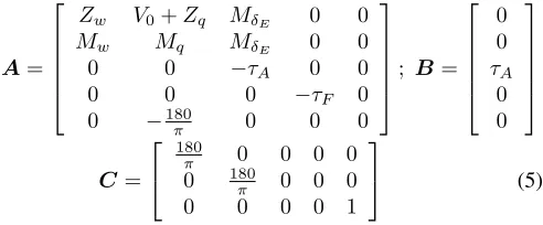
where the state vector is x = (α, q, δE, αF, ε)T, while the only input variable is the pitch velocity reference signal rq. Provided that the output variables are y = (α, q, ε)T, the state, control, and output matrices are defined as
A=
⎡ ⎢ ⎢ ⎢ ⎢ ⎣
Zw V0+Zq MδE 0 0
Mw Mq MδE 0 0
0 0 −τA 0 0
0 0 0 −τF 0
0 −180π 0 0 0
⎤ ⎥ ⎥ ⎥ ⎥
⎦; B=
⎡ ⎢ ⎢ ⎢ ⎢ ⎣
0 0
τA
0 0
⎤ ⎥ ⎥ ⎥ ⎥ ⎦
C=
⎡ ⎣
180
π 0 0 0 0
0 180π 0 0 0 0 0 0 0 1
⎤
⎦ (5)
respectively. The gains of the stability augmentation system (Kα andKq) and the integral gain (Ki) will be determined by means of an optimization algorithm in the framework of the H∞ control theory.
C. Robust control
Consider the system depicted in Fig. 2, where P0(s) is
the nominal model of a plant withniinputs andnooutputs,
C(s)is the controller,r(s)is the reference input signal that needs to be tracked by the output y(s), d is the noise on the output signal and n is the noise on the sensors. Given the definition of the output transfer matrix as Lo =P0C,
the sensitivity at the output is defined as the transfer matrix
y/d, that is
So= (I+Lo)−1, y=Sod (6)
and the complementary sensitivity function at the output is
To=I−So=Lo(I+Lo)−1 (7) From the system represented in Fig. 2, the output can be expressed as
Fig. 2. General feedback configuration with disturbances.
Fig. 3. Feedback configuration with multiplicative uncertainties on the nominal model.
Moreover, apart from external noises affecting the signals, the system may be characterized by other kind of uncer-tainties. Usually, the nominal modelP0 does not correspond to the actual plant, due to simplifying assumptions and/or linearization. Taking into account a multiplicative uncertainty on the plant model (Fig. 3), the following expression for the output is obtained:
y= To+ ΔTo
I+ ΔTo r
(9)
In order to reduce the effect of the uncertainty it is neces-sary to tailor the complementary sensitivity function of the uncertainty itself, ΔTo.
The main idea behind H∞ control theory and the design process derived in this framework is to find the values of the controller parameters by minimizing appropriately the infinite norm of the weighted sensitivity and complementary sensitivity functions. In order to achieve this result, the following functions need to be minimized:
W1(s)So(s)= min ; W3(s)To(s)= min (10) that is, the effects of noise on the output and that of uncer-tainties of the nominal model P0 are reduced, W1(s)and W3(s) being weighting functions chosen during the design
as a function of exptected disturbances and uncertainties and requirements on closed–loop performance.
Since theH∞norm of a systemG(s)is G∞= sup
ω ¯
σ[G(jω)] (11)
where σ¯(·) is the maximum singular value, this kind of norm provides the worse gain for a sinusoidal input at a given frequency, corresponding to the worse energetic gain of the system. The use of weighted functions allows to deal with different kind of signals, when MIMO systems are considered. Moreover, and more important, weights allow to focus the optimisation process only within prescribed
frequency ranges. As an example, in order to reduce low frequency noise a weight function with high gains at low frequency will be used, such that
Wg(s)G(s)∞<1 =⇒ |Gij(s)|< 1 |Wgij(s)|
(12)
that is, the magnitude of each transfer function from inputi to output j is less than the inverse of the magnitude of the corresponding weight.
III. CONTROL LAW SYNTHESIS
As stated in the Introduction, evolutionary optimisation algorithms offer an advantage over gradient based methods, that can hardly be applied when constraints makes the shape of the feasible solution subset of the search space highly irregular. The particular type of evolutionary algorithm used for tackling the considered control problem belongs to the sub–class of Estimation of Distribution Algorithms (EDAs) [9]. In general terms, these methods try to identify a prob-abilistic model of the search space from the results for the current populations. Crossover and mutation operators, typical of classical Genetic Algorithms [8], are replaced with statistical sampling.
A. The evolutionary optimisation algorithm
The MOPED (Multi–Objective Parzen based Estimation of Distribution) algorithm is a multi–objective optimisation algorithm for continuous problems that uses the Parzen method to build a probabilistic representation of Pareto solutions, with multivariate dependencies among variables [4], [2]. Similarly to what was done in [8] for multi–objective Bayesian Optimisation Algorithm (moBOA), some tech-niques of NSGA-II are used to classify promising solutions in the objective space, while new individuals are obtained by sampling from the Parzen model. NSGA-II was identified as a promising base for the algorithm mainly because of its intuitive simplicity coupled with excellent results on many problems.
The Parzen method [4] pursues a non-parametric approach to kernel density estimation and it gives rise to an estimator that converges everywhere to the true Probability Density Function (PDF) in the mean square sense. Should the true PDF be uniformly continuous, the Parzen estimator can also be made uniformly consistent. In short, the method allocates Nind identical kernels (where Nind is the number of individuals of the population of candidate solutions), each one centered on a different element of the sample.
1) Classification and Fitness evaluation: The individuals of the population are classified in a way that favors the most isolated individuals in the objective function space, in the first sub-class (highest dominance) of the first class (best suited with respect to problem constraints). If the problem is characterized bymconstraintsci(x),i= 1,2, ..., m, such that cj(x) = 0 indicates that the j–th constraint is satisfied, the first step in the evaluation of the fitness parameter is the determination of the degree of compatibility of each individual with the constraints. The compatibility, indicated by the symbol cp, is measured as the weighted sum of un-satisfied constraint. Once the value of cpis evaluated for all the individuals, the population is divided in a predetermined number of classes,1+Ncl. TheNbestindividuals that satisfy all the constraints, such that cp = 0, are in the first class. The remainder of the population is divided in the other groups, each one containing an approximately equal number of individuals, given by round(Nind−Nbest)/Ncl.
The second class is formed by those individuals with the lower values of the constraint parameter and the last one by those with the highest values. For each class, individuals are ranked in terms of dominance criterion and crowding distance in the objective function space, using the NSGA-II techniques. After ranking all the individuals of the popu-lation, from the best to the worst one, depending on their belonging to a given class and dominance level and the value of their crowding parameter, a fitness valuef linearly varying from2−α(best individual of the entire population) toα(worst individual), with α∈[0; 1), is assigned to each individual.
2) Building the model and sampling: The fitness value determines the weighting of the kernel for sampling the individuals of the next generation. As an example, forα= 0, the best solution (f = 2) provides a kernel with twice as much possibilities of generating new individuals for the next generation than the central one, placed at half of the classification (for a corresponding value off = 1), while the kernel for the worst one (f = 0) is prevented from generating new individuals.
By means of the Parzen method, a probabilistic model of the promising search space portion is thus built on the basis of the information given byNind individuals of the current population, andτNind new individuals (τ≥1) can then be sampled . The variance associated to each kernel depends on (i) the distribution of the individuals in the search space and (ii) the fitness value associated to the pertinent individual, so as to favor sampling in the neighborhood of the most promising solutions. In order to improve the exploration of the search space it is sometimes useful to alternatively adopt two different kernels when passing from one generation to the following one.
3) Algorithm parameters: The parameters to be set for the MOPED algorithm are: size of the population, Nind, number of constraint classes, Ncl, the fitness parameter, α, the sampling proportion,τ. In all the optimisation processes for the present study, the following parameter values were
used: Nind = 100, NgenM AX = 100, Ncl = Nind/10;
α= 0.5;τ = 1.
B. Statement of the optimisation problems
1) S.O. Problem: The single–objective optimisation pro-cess is aimed at minimizing the function F, equal to a weighted sum of the sensitivity and complementary sensi-tivity functions. The objective function is thus expressed as
F =W1(s)S(s)∞+W3(s)T(s)∞ (13)
The weight functions are
W1= s+ 100
100s+ 1; W3=
100s+ 10
s+ 1000 (14)
where W1 is chosen so that the action on the sensitivity function is emphasized in the low frequency range, where the effect of disturbances may affect aircraft performance, while
W3is tailored on the basis of assumed characteristics for the
uncertainties on the nominal model of the plant. Sensitivity, complementary sensitivity and weights are scalar functions for the considered SISO problem.
The design variables are the three gains of the SCAS (Fig. 1), namely Kα, Kq, and Ki. The result-ing 3–dimensional search domain is bounded by lb = (−5,−5,−5)T and ub = (0,0,0)T. However, the search space is normalized and the solver operates in the cube
[0,1]×[0,1]×[0,1]⊂R3.
Constraints on peak timetp, settling timetsand overshoot
Mp are also included, representative of requirements on handling qualities. Feasible solutions must thus satisfy the following inequality constraints
tp ≤1s; ts≤3s; Mp≤0.05 (15)
The S.O. problems was first solved on a denser set of trim points, between those tested in [10], and a gain scheduled controller was thus developed. A more detailed analysis was then performed for two pairs of trim points at h = 0 and
h= 12,000ft, each pair corresponding to the minimum and maximum values of the dynamic pressure, respectively.
2) M.O. Problem: In the second approach, a bi–objective optimisation process is carried out for each pair of points with the same dynamic pressure. In this case the solver searches for solutions which optimise the objective functions
F1andF2simultaneously for the two considered trim points,
while enforcing the time–domain constraints for both of them.
IV. RESULTS
200 300 400 500 600 700 800 900 0
2000 4000 6000 8000 10000 12000
A1
A2 B2
B1
V [ft/s]
h [ft]
Vmin
VTmin
Fig. 4. Control law design and test trim points in the F–16 flight envelope.
A. Gain scheduling
The study reported in [10] demonstrated that it is not possible to devise a single set of values for the control gains, Ki, Kα, and Kq, with adequate performance over a large portion of the flight envelope. By exploiting the multi– objective approach, the minimization problem was simulta-neously considered at three different trim conditions (low, medium and high speed at increasing altitudes, x symbols in Fig. 4), but the strong variation of the control derivative
MδE with the dynamic pressure prevents the algorithm from finding a compromise between high control power (and resulting small deflections) at high speed and weaker control effectiveness at low speed.
When the nominal values of the time–domain constraints were considered, it was not possible to simultaneously drive the optimisation process to convergence with an H∞ norm less than 1 in all the design points and, viceversa, for those values of Ki, Kα, and Kq resulting in a robust controller, time–domain requirements where violated at least for one of the design trim conditions. Only by relaxing time–domain constraints, thus allowing a higher overshoot and/or a longer rise–time, an acceptable controller that satisfies the necessary condition for robustness was obtained. These results were further confirmed by analysis of the closed–loop system response to a step input in the test points (+ symbols in Fig. 4).
After the preliminary application described in [10], a more detailed analysis of the variation of controller gains for different values of the scheduling parameter Q was performed. A set of 9 design points was selected (•symbols in Fig. 4) and the optimal gains were identified by means of a single–objective evolutionary optimisation process. Note that all the points lie in the region where thrust necessary for level flight increases with velocity (that is, to the right of the minimum–thrust trim flight condition in the h–V flight envelope), in a range of altitudes between sea level and approximately 1/4 of the aircraft service ceiling, rated around 50,000 ft. The considered analysis will be limited
300 350 400 450 500 550 600 650 −1.8
−1.6 −1.4 −1.2 −1 −0.8 −0.6 −0.4 −0.2 0
Q [psf]
gains
Ki
Kα
Kq
Fig. 5. Control law design and test trim points in the F–16 flight envelope.
to the subsonic velocity range, as compressibility effects are neglected by the aircraft aerodynamic model.
The variation of the obtained controlled gains is relatively smooth, as shown in Fig. 5. The stability augmentation system needs an almost constant gain Kα throughout the considered interval ofQ, while significant adjustments to the pitch–damper and command augmentation gainsKq andKi are required. Both Kq and Ki are almost exactly inversely proportional with respect to Q: a variation from −0.56 to −0.24 is required for Kq, and between −1.72 and −0.75 for Ki, with a ratio equal to 2.33 for the first one and 2.29 for the second, that almost exactly matches the ratio
Qmax/Qmin= 2.24.
This type of variation can be explained on physical grounds, when one considers that the angle of attack α remains well within the linear aerodynamic range, through-out the considered portion of the flight envelope, and the variation of the gains is mainly driven by control power, which is proportional to the dynamic pressure Q. In this framework a robust controller can handle the variations of the dynamic response when aggressive manoeuvres are considered, involving the nonlinear terms of the complete aerodynamic model when large variation ofαare considered.
B. Effects of altitude changes for fixed values ofQ
In order to evaluate the effects of altitude changes for fixed values ofQ, four design trim conditions for the F–16 aircraft model were considered (listed in Table I and indicated in Fig. 4 as A1, A2, B1, and B2). Three additional trim conditions were used for simulation of the closed–loop behaviour in off–nominal conditions (T1, T2, and T3 in Table I).
[image:6.595.318.549.54.235.2] [image:6.595.53.278.64.232.2]TABLE I TRIM CONDITIONS
V [ft/s] h[ft] Q[psf]
A1 500 0 297
A2 600 12 000 297
B1 748 0 666
B2 900 12 000 666
T1 736 24 000 297
T2 821 30 000 297
T3 700 6 000 486
0.82 0.84 0.86 0.88
0.84 0.85 0.86 0.87 0.88 0.89 0.9 0.91 0.92
F (h = 0)
F (h > 0)
CA1 check in A2 CA1 check in T1 CA1 check in T2 CA2 check in A1 CA12
CB1 check in B2 CB2 check in B1 CB12
Fig. 6. Pareto front approximations and cross-checking
and CB2 are the controllers optimized in B1 and B2 trim points, respectively, while CB12 is one of the controllers obtained when B1 and B2 flight conditions are considered simultaneously.
The analysis of the results and the cross checking of the controller behaviour in off-design conditions show that controller scheduling over dynamic pressure may not be sufficient for robust performance and handling qualities, as far as speed and altitude may play a role separately. In particular, if the low dynamic pressure range is considered, controller CA1 behaves well (in terms of both frequency and time domain constraints) also in A2 (even if the rise time increases and the constraints are enforced only marginally). As a matter of fact, the small pareto front in Fig. 6 (+signs) obtained when A1 and A2 conditions are considered together starts from the point corresponding to CA1. It should be noted that the opposite is not true, that is, CA2 fails to work in A1, since the rise time constraint is violated. Moreover, if altitude is further increased (points T1 and T2, not reported in Fig. 4), also the behaviour of CA1 becomes less and less acceptable, with more sizable violation of the constraint on the overshoot, induced by the reduction of the damping when density gets smaller.
The importance of considering the influence of altitude for a given value ofQappears even more evident when high dy-namic pressure conditions are taken into account. Both CB1 and CB2 controllers do not satisfy time domain constraints when checked in the other design point. The difficulties of the control synthesis for high values ofQare also highlighted
TABLE II
CROSS-CHECKING OF CONTROLLERS AND TRIM CONDITIONS:TIME
CONSTRAINTStp,Mp,ANDts
tp Mp ts
CA1 in A2 0.990802 0.042508 2.732465 CA1 in T1 0.955337 0.053440 2.750411 CA1 in T2 0.946109 0.058752 2.419744 CA2 in A1 1.121142 0.021026 2.703230 CB1 in B2 1.036109 0.031622 2.635621 CB2 in B1 0.954420 0.071994 3.147958
by the results of the Pareto front related to the search for the CB12 control. In this case the solver is not able to spread the population over a front of feasible solutions, rather, it finds a single feasible solution which satisfies constraints in both the design points, but it is characterized by a weaker rubustness in both points, if compared with CB1 and CB2.
In order to further validate the approach, a final check was performed in the trim point T3, which has an interme-diate value of Q between Qmin and Qmax. The controller obtained by linear interpolation between CA12 and CB12 gives following values: W1S = 0.17134, W3T = 0.77243,
tp = 1.03042, Mp = 0.01019, and ts = 2.93653, which means that all the design requirements are met, with only a marginal violation for the rise time, thus confirming on one side the effectiveness of the scheduling method, but at the same time the importance of including the effects of altitude on the model during the design phase.
C. Nonlinear simulation
As a final check for the validity of the proposed approach, a set of simulations was performed, based on the complete longitudinal model, thus including the effects of velocity and climb angle variations on closed–loop response, which were not accounted for in the design phase, where only a reduced– order short–period model was considered. Moreover, the nonlinear aerodynamic model, where aerodynamic coeffi-cients are tabulated as a function of aerodynamic angles and control surface deflection, further challenges the robustness of the SCAS, when aggressive manoeuvres are simulated, with large variations of α. Two manoeuvres were tested, starting from the same trim condition, namely T3, in order to consider an off–design reference point.
When a unity step on the input channel is considered (Fig. 7), the resulting manoeuvres involves a mild variation of pitch angular velocity and angle of attack. The behaviour of the nonlinear model resembles almost perfectly that of the linear one, used for the synthesis process. In the short term, rise and settling times and overshoot matches the values obtained for the linear case, and only minor differences are present at the end, because of the reduction of velocity and increase in the flight–path angle,γ.
0 1 2 3 4 5 6 590
595 600 605
V [fps]
0 1 2 3 4 5 6
0 2 4
α
,
θ
,
γ
[deg]
α γ θ
0 1 2 3 4 5 6
0 0.5 1 1.5
q [deg/s]
[image:8.595.64.278.75.314.2]t [s]
Fig. 7. Nonlinear model response to a step input (rq= 1deg/s).
0 5 10 15 20
400 500 600
V [fps]
0 5 10 15 20
0 20 40
α
,
θ
,
γ
[deg]
α γ θ
0 5 10 15 20
−10 0 10
q [deg/s]
[image:8.595.63.279.244.420.2]t [s]
Fig. 8. Nonlinear model response to a double impulse (rq= 10deg/s).
20 seconds in order to evaluate the recovery capabilities of the SCAS, with no further pilot input.
In the first phase (t <6s), the sudden increase of the angle of attack of almost 10 deg puts the aicraft on a steep climbing trajectory, so that the velocity rapidly drops, because the manoeuvre was not accompanied by a change in the throttle setting. In spite of this, the command augmentation system succesfully tracks the desired value. After 5 s spent at 10 deg/s of pitch rate, the pitch and climb angles are both around 40 deg, the pitch angle being larger.
At this point the command is reversed. Again, the desired variation of q is succesfully tracked. The higher overshoot clearly visible at 8 s is related to the variation of stability derivatives over an excursion of α, which varies from more than 10 deg to less than -5 in less than 2 s. Nonetheless, when the pitch command is brought bacl to 0, the SCAS succesfully start a recovery phase, which ends at the original trim state without requiring any pilot input.
V. CONCLUSIONS
An evolutionary optimisation technique was adopted as a means for control gain synthesis in the framework of
H∞ control problems. Two different approaches were ana-lyzed: a) a single–objective constrained optimisation process, where the weighted combination of the infinite–norm of
the sensitivity and complementary sensitivity functions were minimized, with constraints on time domain responces, for different trim point conditions; and b) a bi–objective search where a front of optimal feasible solutions is sought, in order to minimize simultaneously the weighted combination of the sensitivity and complementary sensitivity functions for two different flight conditions corresponding to the same value of the dynamic pressure at different flight altitudes.
The results obtained confirm that the evolutionary ap-proach has an advantage over the more traditional LMI control synthesis technique as it is possible to address time– domain constaints during the synthesis of the control law rather than by means of a trial–and–error technique based on a–posteriori simulations. More important, once the relevance of stability derivative variation at different altitudes for a fixed value of the scheduling parameter Q is recongized, the bi–objective approach allows for the determination of controllers which perform extremely well in off–nominal conditions, a result which is impossible to obtain by means of control approaches based on local information only, and confirmed by means of direct simulation of a complete longitudinal nonlinear aircraft model. The only limit of the present study lies in the relatively limited portion of the flight envelope included in the analysis.
The next step of the research will be the development of a full–envelope stability and control augmentation system, based on a set of scheduled gains synthesized over a wider interval on the altitude axis and the application of the technique to more demanding MIMO control tasks, such as a lateral–directional stability and control augmentation system.
REFERENCES
[1] Abzug, M.J., and Larabee, E.E.,Airplane stability and control: a history of the technologies that made aviation possible, Cambridge University Press, 1997.
[2] Avanzini, G., Biamonti, D., and Minisci, E. A., Minimum-fuel/minimum-time maneuvers of formation flying satellites. Adv. As-tronaut. Sci., 2003, 116(III), 2403–2422.
[3] Avanzini, G., and Galeani, S., Robust Antiwindup for Manual Flight Control of an Unstable Aircraft. J. of Guidance, Control and Dynamics, 28(6), 2005, 1275-1282.
[4] Costa, M., and Minisci, E., MOPED: a multi-objective Parzen-based estimation of distribution algorithm. In Proc. of EMO 2003, Faro, 2003, 282-294.
[5] Droste, C.S.,The general dynamics case study on the F16 fly– by–wire flight control system, AIAA Professional Series, New York, 1985. [6] Etkin, B.,Dynamics of atmospheric flight, J. Wiley, New York, 1972. [7] Francis, B.A., A course inH∞control theory, Lecture Notes in Control
and Information Sciences, Vol. 88, Springer-Verlag, Berlin, 1987. [8] Khan, N., Golberg, D.E., and Pelikan, M., “Multi-objective Bayesian
Optimisation Algorithm”, Technical Report IlliGAL 2002009, Univer-sity of Illinois at Urbana-Champain - IlliGAL, 2002.
[9] Larra˜naga, P., and Lozano, J.A.,Estimation of Distribution Algorithms. A New Tool for Evolutionary Computation, Kluwer Academic Publish-ers, 2002.
[10] Minisci, E.A., Avanzini, G., D’Angelo, S., and Dutto, M., Multi– Objective Design of Robust Flight Control Systems, ICNPAA 2008 (Mathematical Problems in Engineering, Aerospace and Sciences), Genova (Italy), 25-27 June 2008.
[11] Mitchell, M.,An Introduction to Genetic Algorithms, The MITPress, 1998.
[12] Stevens, B.L., and Lewis, F.L.,Aircraft Control and Simulation, Wiley, New York, 1992.