Application of a new multi-agent Hybrid Co-evolution based Particle Swarm Optimisation methodology in ship design

(1)

APPLICATION OF A NEW MULTI-AGENT BASED PARTICLE SWARM OPTIMISATION METHODOLOGY IN SHIP DESIGN

HAO CUI and OSMAN TURAN

Department of Naval Architecture and Marine Engineering, Universities of Glasgow and Strathclyde, Glasgow, G4 0LZ, United Kingdom

ABSTRACT

In this paper, a multiple objective ‘Hybrid Co-evolution based Particle Swarm Optimisation’ methodology (HCPSO) is proposed. This methodology is able to handle multiple objective optimisation problems in the area of ship design, where the simultaneous optimisation of several conflicting objectives is considered. The proposed method is a hybrid technique that merges the features of co-evolution and Nash equilibrium with ε-disturbance technique to eliminate the stagnation. The method also offers a way to identify an efficient set of Pareto (conflicting) designs and to select a preferred solution amongst these designs. The combination of co-evolution approach and Nash-optima contributes to HCPSO by utilising faster search and evolution characteristics. The design search is performed within a multi-agent design framework to facilitate distributed synchronous cooperation. The most widely used test functions from the formal literature of multiple objectives optimisation are utilised to test HCPSO. In addition, a real case study, the internal subdivision problem of a ROPAX vessel, is provided to exemplify the applicability of the developed method.

Keywords:

Optimisation, Particle Swarm Optimisation, Ship Design, Multi-Agent, ε-disturbance

1．Introduction

Ship design is a dynamic process, and in recent years the multi-objective optimisation in ship design has attracted a lot of interest. In ship design, the internal hull subdivision is very important for damage stability, survivability and cargo capacity performance, particularly for Roll-on/Roll-off (ROPAX) passenger vessels, which have to comply with SOLAS standards, including SOLAS 90 and ‘water on deck’, which is known as the Stockholm Agreement. In order to satisfy these strict regulations, the ship designer needs to optimise the hull subdivision to achieve high safety standards, while improving the capacity and performance of the ship, by utilising a simple and effective method.

(2)

used a GA with Pareto ranking for naval ship concept design. Two objectives were considered: maximize overall measure of effectiveness (this factor represents customer requirements and relates ship measures of performance to mission effectiveness) and minimize life cycle cost. Binary representation and roulette wheel selection with stochastic universal sampling were used. Brown and Salcedo [5, 6] introduced a Multi-Objective Genetic Algorithm in naval ship design. Todd and Sen [7] used a variant of MOGA for the pre-planning of containership layouts (a large scale combinatorial problem). Four objectives were considered: maximize proximity of containers, minimize transverse center of gravity, minimize vertical center of gravity, and minimize unloading. Binary representation and roulette wheel selection with elitism based on non-dominance were used. They used the same algorithm for the cutting shop problem in the shipyard [8], [9]. Two objectives were considered: minimize makespan and minimize total penalty costs. Peri and Campana [10] proposed a multidisciplinary design optimisation of a naval surface combatant and also developed High-Fidelity Models and Multi-Objective Global Optimisation Algorithms in Simulation-Based Design [11]. Olcer [12] proposed a hybrid approach for multi-objective optimisation problems in ship design and shipping. In his study, software ‘Frontier’ was used to perform optimisation via MOGA. Boulougouris and Papanikolaou [13] introduced a multi-objective optimisation of a floating LNG terminal. The software ‘Frontier’ with MOGA was utilized.

The Particle Swarm Optimisation (PSO) algorithm, which was proposed by J.Kennedy and R. Eberhart in 1995 [14], has been successfully used in single-objective optimisation problems. Since Moore and Chapman [15] proposed the first extension of the PSO strategy for solving multi-objective problems in 1999, a great deal of interest has been shown in multi-objective optimisation and many different approaches/techniques have been presented in literature. PSO, which has been successfully applied in numerous engineering areas, has only a small number of parameters, which need to be adjusted and is easy to implement.

In ship design, Pinto et al. [16] emphasised the importance of initial points’ configuration and addressed some preliminary aspects of global convergence of PSO towards stationary points. In their follow-up paper [17], they presented a deterministic method for multi-PSO and applied the method to the multi-objective (two objectives) seakeeping of containership problem.

Since Mistree [18] approached ship design from a decision perspective, the decision making based ship design environment has developed rapidly. In recent years, multi-agent based ship design decision making has received a great deal of attention and at the same time the distributed synchronous cooperative ship design method via the internet is becoming a new research field. However, in terms of simplicity and efficiency, it requires a new optimisation approach which is suitable for a multi-agent system.

(3)

The paper is organised as follows: Section 2 presents PSO and Multi Objective Particle Swarm Optimisation (MOPSO), and Section 3 presents a new multi-objective particle swarm optimisation methodology and the detailed explanation of this algorithm. the test functions are processed in section 4, while a real case study ‘hull subdivision design optimisation’ is performed in section 5. Finally, in section 6, discussions and conclusions are presented.

2. Background

The Particle Swarm Optimisation is a global optimisation algorithm and described as sociologically inspired. It was first proposed by Kennedy and Eberhard in 1995 [14]. In the PSO algorithm, the candidate solution is the particle position in search space. Every particle is structured with two parameters: position and velocity, then the particle searches the solution space by updating the position and velocity. There are two best positions in PSO. The first one is Pbest, which represents the best position that the particle itself can reach; the other is Gbest, which is the best position in the whole swarm.

The PSO can be described as following,

1

1 1 2 2

1 1

( ) (

;

n n n n n n n n

id id id id gd id

n n n

id id id

v v c r p x c r p x

x x v

ω

χ

+ + + = + − + − = + ); (1)

where x_idn is the position of particle i, in n-th iteration and d dimension; is the velocity of particle i,

in n-th iteration and d dimension; as Pbest is the best position of particle reached and

n id v n id p n gd

p

as

Gbest is the best position in current swarm; and are two coefficients; and are two random numbers with the range [0,1];

1

c

₂

r

₁

r

₂

ω

is the inertia weight and

χ

is the constriction factor.

PSO has been proven as a simple but effective algorithm in single objective optimisation and multi-objective research has rapidly developed in recent years. Since the first extension was proposed in 1999, many different multi-objective PSOs have been presented [19] and some of these approaches are briefly given below.

Aggregating approaches: They combine all the objectives of the problem into a single objective and

three types of aggregating functions are adopted: conventional linear aggregating function, dynamic aggregating function and the Bang-bang weighted aggregation approach (Parsopoulos and Vrahatis [20], Baumgartner et al.[21] and Jin et al [22]).

Lexicographic ordering: In this algorithm, which was introduced by Hu and Eberh [23], only one

objective is optimized at a time using lexicographic ordering Schema.

Sub-Population approaches: These approaches involve the use of several subpopulations as

(4)

previously generated for the objectives that were individually optimised. Parsopoulos et al. [24], Chow et al.[25] and Zheng et al.[26] use this approach.

Pareto-based approaches: These approaches use leader selection techniques based on Pareto

dominance and references include Moore and Chapman [27], Ray and Liew [28], Fieldsend and Singh [29], Coello et al [30] and [31] and Li [32].

Some of the other approaches, which use different techniques such as Combined Approach and

MaxMin approach, can also be found in literature.

Sefrioui and Periaux [33] introduced Nash equilibrium of game theory into the multi-objective optimisation. Nash equilibrium is a set of strategies with the property that no player can benefit by changing its strategy while the other players keep their strategies unchanged. A Nash genetic algorithmwas given with comparisons to Pareto GAs. They concluded that Nash genetic algorithms offer a fast and robust alternative for multi-objective optimisation.

3. Description of the Proposed Approach - HCPSO

The proposed approach combines co-evolution approach, Nash equilibrium and ε-disturbance technique to form a new improved hybrid approach. At the same time, the agent-based structure is adopted for distributed synchronous cooperation.

In HCPSO, the co-evolution approach is combined with Nash optima, which looks for Nash Equilibrium. For an optimisation problem with M number of objectives in an agent environment, M numbers of agent-groups are employed to optimise their own objective while changing the objective of other/remaining agent-groups. When no agent-group can improve its objective further, it means that the system has reached a state of equilibrium called Nash Equilibrium. In HCPSO, the co-evolution approach provides a public information sharing mechanism to improve the communication amongst agent-groups.

The reason for adopting the co-evolution approach here is that on the one hand, the co-evolution approach can provide quicker search ability, and on the other hand, by using the co-evolution approach it is easier to perform simulation via a multi-agent system. In an engineering application, the approach can be studied in a multi-computer environment thereby reducing the time via parallel calculation.

The Nash optima [33] and [34] is deployed in HCPSO because the information sharing in Nash optima is simple and effective. Furthermore, in Nash optima, one agent, which has one objective, receives the information from other agents, and this is a good model for the multi-agent system in concept and computer realization.

(5)

jump out of the stagnation point. For a given step T, if the stagnant step ts > T, a random ε-disturbance is introduced to both Pbest and Gbest. For example, setting T=10 steps, the algorithm would check the value of Pbest and Gbest at every step. If both Pbest and Gbest keep the same values as the last step, the counter in algorithm will increase by one. In the next iteration, if both Pbest and Gbest still keep the same values, the counter will further increase by one, otherwise the counter returns to zero. When the counter is equal to 10, the algorithm will give a random ε-disturbance value to change Pbest and Gbest, so as to keep the particles moving.

For an optimisation problem with K design variables and M objectives, the algorithm would employ N particles to run optimisation and N should be multiples of M. Firstly, HCPSO divides N particles into M sub-swarm group according to objectives. Secondly, the design variables, K, are also divided into K1, K2, … Km sub-groups according to the objectives. This means every sub-swarm group has its

own corresponding objectives and design variables. Then every sub-swarm group optimises relevant design variables according to relevant objectives in its own group. The optimised result would be sent to the “public board” as shared information. In the next step, the sub-swarm group would read other design variables and corresponding information from the public board as an update. At last, when a Nash Equilibrium is reached, the algorithm gives the final results. In every sub-swarm, in order to give enough pressure to push the solution space to Pareto space, particles in two generations are compared to update the position.

Algorithm HCPSO

The step-wise description of the proposed algorithm, HCPSO, is given below and shown in Fig.1: 1. initialize the population including position and velocity;

(i) create a public-board to store information; the public-board is a simple database to store all particles’ information;

(ii) give the number of sub-swarms and size of each sub-swarm; (iii) divide the population into sub-swarms;

2. every sub-swarm begins iteration; for example (mth sub-swarm with (N/M) particles and Km design

variables);

3. read information from public-board and calculate fitness;

4. update Pbest via comparing individual position history according to mth_{objective ;}

5. non-dominated sorting via Pareto-based approach;

6. give pointed number of best ranking particles to the public-board;

7. collect particles in step 6 from all sub-swarm to the public-board and form Gbest pool; 8. every sub-swam randomly selects Gbest from the pool;

9. compare Pbest and Gbest with past values to decide whether to introduce ε-disturbance or not; 10. calculate velocity and give limit velocity;

11. update and limit the position of particles;

12. combine last iteration particles with this iteration to form a new group with 2*(N/M) population and perform non-dominated sorting via Pareto-based approach;

13. select first (N/M) particles from new group with 2*(N/M) population in step 12 and update position and velocity;

14. send corresponding information to the public-board;

(6)

16. output final results;

Sub-swarm partition

In HCPSO, the whole swarm is divided into different sub-swarms according to the number of objectives. If an optimisation problem has M objectives, the swarm is divided in to M sub-swarms. The relationship between variable and sub-swarm is very important. For special objective functions, detailed analysis of these relationships should be processed before the partition. For example, a two objective problem:

f x

₁

( )

=

x f x

₁

, ( )

₂

=

g x x

( , ,..., );

₂ ₃

x

_n , following the above principle, the swarm should be divided into two sub-swarms. The first choice of variables is allocated to the first sub-swarm which contains variable

x

₁and second sub-swarm includes the variables from

x

₂ tox_n. The second choice is averaged out and every sub-swarm has half variables. In a particle application in engineering, when the relationship is unclear, the averagedistributionis recommended.

Information sharing mechanism

The information sharing mechanism is realised through a public-board in sub-swarm optimisation. The public-board concept in HCPSO comes from a multi-agent system environment. For easy and efficient communication in an agent environment, a black board is used for sharing the public information. The same mechanism is used here, and the black board is called a public board for public information sharing. In every sub-swarm, the particles optimise variables according to the sub-swarm optimisation objective, and send the information, including the optimised objective value, the best particle location etc. to the public board in the system. In synchronization, the sub-swarm reads the information from the other sub-swarm optimisation as the information for the next step.

Pbest and Gbest updating

The Pbest updating in HCPSO adopts the updating inside sub-swarm while Gbest uses updating outside sub-swarm. For Pbest, the particle in nth sub-swarm compares the corresponding objective fitness value between the current position and the previous best position. If the current position in the nth_{objective fitness is better than the previous value, the Pbest is replaced by the current value or if}

the current value is not better, then the previous value is retained.

The Gbest selection uses the Gbest pool in the public board. Every sub-swarm provides its best value to the public board and constructs a Gbest pool. HCPSO randomly selects a particle as the Gbest position from the Gbest pool.

Particle updating

(7)

[image:7.595.100.457.67.749.2]

(8)

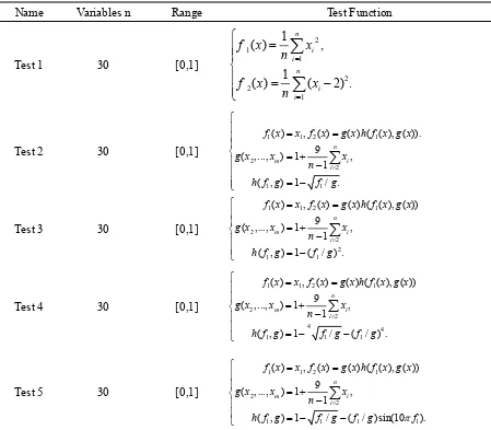
4 Experiments 4. 1 Test Functions

[image:8.595.72.521.320.713.2]

From the related literature, eight multi-objective test functions (Table1) ,are selected to evaluate this algorithm. Deb [35] introduced the design of a multi-objective test problem for EAs (Evolutionary Algorithms) and the test problems in Table 1 are chosen following the principles of Deb. Test 1 is selected by Pinto etc. [17] as a convex Pareto front. Test 2 is ZDT1 function in Zitzler etc. [36] with continuous Pareto front and a uniform distribution of solutions across the front. Test 3 is ZDT2 in which the Pareto front is not convex. Test 4 is obtained combining the test function of Test 2 and Test 3 (Jin et al. 2001) and explored by Pinto etc. [17]. Test 4 is neither purely convex nor purely non convex. Test 5 is ZTD3, which is difficult for a discontinuous Pareto front. Test 6 is ZTD4 and the difficulty of this problem is that the sheer number of multiple local Pareto-optimal fronts produce a large number of hurdles for an algorithm to converge to the global Pareto-optimal front.

Table 1

Two-objective test problems selected to evaluate HCPSO algorithm.

Name Variables n Range Test Function

Test 1 30 [0,1]

2 1 1 2 2 1 1 ( ) , 1

( ) ( 2) .

n i i n i i

f x x

n

f x x

n = = ⎧ ₌ ⎪⎪ ⎨ ⎪ ₌ ₋ ⎪⎩

∑

Test 2 30 [0,1]

1 1 2 1

2

1 1

( ) , ( ) ( ) ( ( ), ( )). 9

( ,..., ) 1 , 1 ( , ) 1 / .

n

m i

i

f x x f x g x h f x g x

g x x x

n h f g f g

= ⎧ ⎪ ₌ ₌ ⎪⎪ ⎨ _{= +} ⎪ ₋ ⎪ = − ⎪⎩

∑

Test 3 30 [0,1]

1 1 2 1

2 2 2 1 1 ( ) , ( ) ( ) ( ( ), ( )) 9

( ,..., ) 1 , 1 ( , ) 1 ( / ) .

n

m i

i

g x x x

n h f g f g

= ⎧ = = ⎪ ⎪ _{= +} ⎨ ₋ ⎪ ⎪ _{= −} ⎩

∑

Test 4 30 [0,1]

1 1 2 1

2

4 ₄

1 1 1

( ) , ( ) ( ) ( ( ), ( )) 9

( ,..., ) 1 , 1

( , ) 1 / ( / ) .

n

m i

i

g x x x

n

h f g f g f g

= ⎧ ₌ ₌ ⎪ ⎪ = + ⎨ ₋ ⎪ ⎪ _{= −} ₋ ⎩

∑

Test 5 30 [0,1]

1 1 2 1

2

1 1 1

( ) , ( ) ( ) ( ( ), ( )) 9

( ,..., ) 1 , 1

( , ) 1 / ( / )sin(10 ).

n

m i

i

1

g x x x

n

h f g f g f g πf

(9)

Test 6 10 1 [0,1], [ 5,5], 2,...30; x xi i ∈ ∈ − =

1 1 2 1

2 2

2

1 1

( ) , ( ) ( ) ( ( ), ( ))

( ,..., ) 1 10( 1) ( 10cos(4 )),

( , ) 1 / .

n

m i

i

g x x n x x

h f g f g

π = ⎧ ₌ ₌ ⎪ ⎪ _{= +} _{− +} ₋ ⎨ ⎪ ⎪ _{= −} ⎩

∑

Two three-objective test functions are selected according to Deb [37] in Table 2. Test 7 is DTLZ2 and is used here to investigate HCPSO’s ability to scale up its performance in a large number of objectives. Test 8, as DTLZ4, is selected to test HCPSO’s ability to maintain a good distribution of solutions.

Table 2

Three-objective test problems selected to evaluate HCPSO algorithm.

Name Variables n Range Test Function

Test 7 12 [0,1]

1 1

2 1

3 1

2

( ) (1

(

)) cos(

/ 2) cos(

/ 2)

( ) (1

(

)) cos(

/ 2)sin(

/ 2)

( ) (1

(

))sin(

/ 2)

(

)

(

0.5)

i M M M M M i x x

f x

g x

x

f x

g x

x

f x

g x

x

g x

x

π

∈

= +

⎧

⎪

_{= +}

⎪

⎨

= +

⎪

=

−

⎪

⎩

∑

2 2

Test 8 12 [0,1]

100 100 1 1 100 100 2 1 100 3 1 2

( ) (1

(

)) cos(

/ 2) cos(

/ 2)

( ) (1

(

)) cos(

/ 2)sin(

/ 2)

( ) (1

(

))sin(

/ 2)

(

)

(

0.5)

i M M M M M i x x

f x

g x

x

f x

g x

x

f x

g x

x

g x

x

π

∈

⎧

= +

⎪

= +

⎪⎪

⎨

_{= +}

⎪

=

−

⎪⎩

∑

2 2

4.2 Parameters Setting

As a critical parameter for the PSO’s convergence behaviour,

ω

is utilised to control the impact of prior velocities. Usually, a large

ω

facilitates global exploration while a small one tends to facilitate local exploration. The experimental results indicate that it is better to set the inertia to a large value initially, in order to promote global exploration of the search space, and gradually decrease it in order to obtain more refined solutions. The proper setting of parameters c1 and c2 may result in faster convergence and alleviation of local minima. The constriction factor χcontrols the magnitude of the velocities, in a similar way to the Vmax parameter. (Parsopoulos and Vrahatis [38])

The standard PSO is the original algorithm provided by

Kennedy and Eberhard (literature?), which is similar to equation (1) but without

χ

. The coefficient

ω

is equal to 1 and

c

₁

=

c

₂

=

2.0

.

In order to perform a comparison with regards to the rate of convergence between standard

PSO and its improved form, two test functions in the literature are selected[39][40]:

[image:9.595.70.528.260.469.2]

(10)

2 1

( )

n i

f x =

∑

x

,

−

5.12 ≤ ≤

x

_i

5.12 Global minimum

f x( ) 0=

is obtainable for

x

_i₌₀

,

i

=

1,..., .

n

2. Griewangk’s function

2

1 1

1

( ) cos( ) 1

4000

n n

i i

x

f x x

i

= =

=

∑

−

∏

+

,

−

600 ≤ ≤

xi

600 2D

2 2

( , )

cos( ) cos(

) 1

4000

2 x

y

f x y

=

+

−

x

+

Global minimum (x,y)=(0,0)

f =0;

For a better and more comprehensive comparison of the rate of convergence, the Genetic

Algorithms (GA) are also included in the comparison, and the parameters used for each

approach are listed in Table 3.

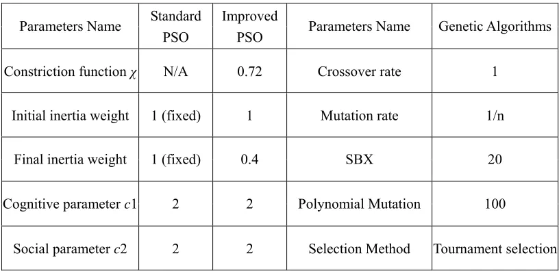
Table 3

The parameters used for standard PSO, improved PSO and GA in comparing

the rate of

convergence

Parameters Name Standard PSO

Improved

PSO Parameters Name Genetic Algorithms

Constriction function χ N/A 0.72 Crossover rate 1

Initial inertia weight 1 (fixed) 1 Mutation rate 1/n

Final inertia weight 1 (fixed) 0.4 SBX 20

Cognitive parameter c1 2 2 Polynomial Mutation 100

Social parameter c2 2 2 Selection Method Tournament selection

[image:10.595.70.478.413.611.2]

(11)

(a) (b)

(c) (d)

Fig.2.

Comparison of the rate of convergence between s

tandard PSO, improved PSO and GA; (a)

De Jong’s function; (b) De Jong’s function with average fitness range from 0 to 1; (c)

Griewangk’s function; (d) Griewangk’s function with average fitness range from 0 to 10;

Typical convergence of average fitness values as a function of generations is shown in Fig.2.

As far as De Jong’s function is concerned, the rate of convergence for standard PSO is better

than GA, but the rate of convergence for the improved PSO is the best among three

algorithms.With regards to Griewangk’s function (Figure (c) and (d)), the improved PSO is

still the best one while GA performs better than standard PSO. The reason for this is that the

standard PSO has to adjust itself through Vmax, which is difficult to control.

Clerc and Kennedy [41] have given a mathematical analysis of algorithm parameters and derived a reasonable set of turning parameters. Based on this, Trela [42] provides a direct and simple guideline for parameter selection. A convergence triangle is given as a diagram (Fig. 3). Trela transfers classic PSO formula to the following and makes c=d=1:

1 1 1 1 2 2 2

1 1

(

)

(

)

;

k k k

v

av

b r p

x

b r p

x

cx

dv

+

+ +

=

+

−

+

−

=

+

;

k ₍₂₎

1 2_;

2

(12)

Corresponding to (1), a and b can be expressed as:

1 2

; (

2

a

c c b

χω

χ

= ⎧ ⎪

⎨ ₌ +

⎪⎩ ) (3)

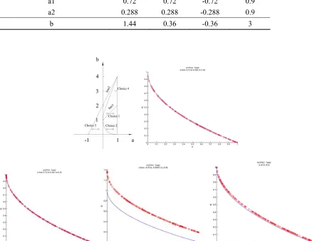
These parameters are critically important for PSO. The different parameters setting is given in Table 4. Test 2 is selected as a standard test function to evaluate the effort of parameters in HCPSO. The number of particles and generation are set to 200 and 50 respectively, in order to compare the final results (Fig. 3).

Table 4

HPSCO parameters used for the comparison of

the rate of convergence on a multi-objective

optimization problem --- Test 2 in Table 1;

Parameters Name Choice 1 Choice 2 Choice 3 Choice 4 Constriction Function χ 0.72 0.72 -0.72 1.5

Initial inertia weight 1 1 1 0.6

Final inertia weight 0.4 0.4 0.4 0.6

Cognitive parameter c1 2 0.5 0.5 2

Social parameter c2 2 0.5 0.5 2

a1 0.72 0.72 -0.72 0.9

a2 0.288 0.288 -0.288 0.9

[image:12.595.72.461.275.419.2]

b 1.44 0.36 -0.36 3

[image:12.595.81.519.377.715.2]

(13)

The line 1 in Fig. 3 is a zigzagging line and line 2 is a harmonic oscillation line. As can be

seen from Fig. 3, choices 1 and 2 fit well after optimisation, but choice 3 and choice 4 can not

fit Pareto solutions. Fig. 3 displays that the principle of Trelea is applicable to HCPSO.

4.3 Performance Metrics

Two evaluation criteria are selected: [35]

(1) GD (Generational Distance) finds an average of the solutions of Q from P* (Q is solution and p* is a known set of the Pareto-optimal)

| | 1/ 1 ( ) | | Q p p i i d GD Q = =

∑

For a two objective problem (p=2), is the Euclidean distance between the solution and nearest member of P*.

i

d

i Q∈

(2) Spread

d Q d

= = = + − Δ = +

∑

d

where

d

can be any distance measured between neighbouring solution and

d

is the mean value of

the above distance measure. The parameter is the distance between the extreme solutions of P* and Q, corresponding to mth objective function.

e m

d

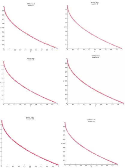
4.3 Results

The HCPSO is run 10 times and real-coded NSGAII, a multi-objective genetic algorithm, is used for comparison. In HCPSO, the parameters are set as following: the population of swarm is 200 and generation is 100 iteration steps.

c

₁ and are set to 0.5 while

c

₂

ω

is gradually decreased from 1.0

to 0.4. Vmax is set to the boundaries of decision variable ranges.

χ

is 0.72. The ε-disturbance has 3 steps. The number of sub-swarm is 2 and population of sub-swarm is 100. In NSGAII, the number of individuals is 200 and the number of generation is set to 100. The SBX (Simulated binary crossover) is used with

η

_c

=

10

and the polynomial mutation is used with

η

_m

=

20

. The crossover and mutation probabilities are set to 0.9 and respectively. The parameters of NSGAII are selected according to prior study, (Turkmen 2005 [43]). The results of performance metrics of Test 1 to 6 are averaged and summarised in Table 5. The non-dominated solutions found by HCPSO for all test functions are

(14)

displayed in Fig. 4 and they all perform very well for both 2D and 3D objectives. The HCPSO gives the last generation results as non-dominated solutions.

Test 1 Test 2

Test 3 Test 4

(15)

[image:15.595.89.512.79.262.2]

Test 7 Test 8

Fig. 4. Non-dominated solutions found by HCPSO on test functions in Table 1 with Pareto Fronts Table 5

Comparison of

mean and variance values of convergence metric GD and diversity metric on six two-objective problems;

Δ

As can be seen in Table 5

，

in comparison to NSGAII, the HCPSO can perform very well for

all six standard multi-objective optimisation test functions, which are tested in this paper.

[image:15.595.103.497.377.630.2]

(16)

(17)

[image:17.595.80.496.69.626.2]

Fig. 5.

Comparison of

convergence history of HCPSO and NSGAII on a

two-objective

optimization problem --- Test 2 in Table 1;

5. Case Study in Ship Design

(18)

off type ships was initiated. The ‘Water on Deck’ standards, which are known as Stockholm Agreement [44] determines the limiting wave height（Hs）in which a ROPAX vessel survives in a damaged condition. In response to these regulations, the shipping industry is in search of new modern designs to match these high safety standards, while maximizing the cargo capacity of vehicles in a cost effective approach.

The changes in design focus on the damage stability and survivability, cargo and passenger capacity. Therefore, the internal hull subdivision layout is an important problem especially for damage stability, survivability, internal cargo capacity and the general arrangement of the vessel.

In literature, different solution methods have been proposed. Sen and Gerick (1992) [45] suggested using a knowledge-based expert system for subdivision design using the probabilistic regulations for passenger ships. Zaraphonitis et al. [46] proposed an approach for the optimisation of Ro-Ro ships in which centre-casing, side-casing, bulkhead deck height and locations of transverse bulkheads are treated as optimisation variables. Ölçer et al. [47] studied the subdivision arrangement problem of a ROPAX vessel and evaluated conflicting designs in a totally crisp environment where all the parameters are deterministic. They also examined the same case study in a fuzzy multiple attributive group decision-making environment, where multiple experts are involved and available assessments are imprecise and deterministic (Ölçer et al. [48]). Turan et al. (2004) [49] approached the subdivision problem by using the case-based reasoning approach. Turkmen et al. (2005) [43] proposed NSGAII with TOPSIS (Technique for Order Preference by Similarity to Ideal Solution) to perform design optimisation for internal subdivision.

5.1 Problem Modelling

The case study naturally focuses on improving the performance of the Ropax vessels in terms of not only maximising the ship related parameters mentioned above but also reducing the time to perform the multi-objective design iteration.

As this study is based on the previous work of Ölçer et al. [47], [48] and Turkmen et al. [50] the same problem is selected and used in this study. The optimisation problem is an internal hull subdivision optimisation for a ROPAX vessel whose main particulars are given in Table 6. Therefore the main aim of this case study is to maximise the survivability and damage stability standards, as well as to improve the cargo capacity. These three parameters form the objectives of the study as presented in Table 7.

The recently developed ‘Static Equivalent Method (SEM)’ [51] is used to calculate the limiting significant wave height (HS) value for the worst SOLAS’90 damage, determined from damage

stability calculations.

(19)

[image:19.595.133.466.243.407.2]

wave height as an equivalent approach. The SEM is an empirical capsize model for Ro-Ro ships that can predict with reasonable accuracy the limiting sea-state for specific damage conditions. The SEM for Ro–Ro ships postulates that the ship capsizes quasi-statically, as a result of an accumulation of a critical mass of water on the vehicle deck, the height of which above the mean sea surface uniquely characterises the ability of the ship to survive in a given critical sea state. This method was developed following observations of the behaviour of damage ship models in waves and it was validated using several model experiments and a large number of numerical simulations. Therefore, in this particular case study, SEM is used as an equivalent approach to the Stockholm Agreement.

Table 6

Main dimensions of the vessel used in the case study.

Length overall(Loa) 194.4 m

Length between perpendiculars (Lbp) 172.2 m

Breadth moulded (B) 28.4 m

Depth to car deck 9.7 m

Lower hold height (m) 2.6 m

Depth to upper deck 15.0 m

Draught design (T) 6.6 m

Displacement 20200 ton

Max number of persons on board 2660

Number of car lanes 8

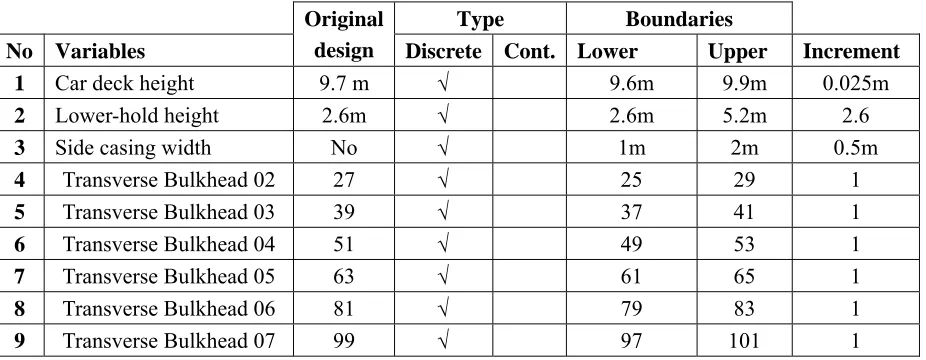
There are three objectives and 16 design variables in this study (Table 7). Three of the design variables are: the depth of the ship to the car deck ’Car Deck Height’, ‘Lower Hold Height’ and the width of the side casing at the car deck, ’Side Casing Width’. As presented, the original design has a 9.7 m depth to car deck, a 2.6 m lower deck height and no side casings at the car deck (Fig. 10 a). The remaining 13 design parameters are the locations of transverse bulkheads given in the format of frame numbers (starting from the stern of the ship). Table 7 also presents the lower and upper boundaries of the parameters with assigned increments to be used in the optimisation study.

Table 7

Optimisation variables with their types, boundaries, and objectives.

Type Boundaries No Variables

Original

design Discrete Cont. Lower Upper Increment

1 Car deck height 9.7 m √ 9.6m 9.9m 0.025m

2 Lower-hold height 2.6m √ 2.6m 5.2m 2.6

3 Side casing width No √ 1m 2m 0.5m

4 Transverse Bulkhead 02 27 √ 25 29 1

[image:19.595.69.532.576.756.2]

(20)

Boundaries for transverse bulkheads are given in frame numbers

No Objectives Type Description

1 HS value Maximization for the worst two compartment damage case

2 KG limiting value Maximization for the worst two compartment damage case 3 Cargo capacity

value

Maximization expressed in car lanes

The damage stability has been calculated according to the constraints of SOLAS’90 regulations as shown in Table 8.

Table 8

Constraints of SOLAS’90 requirements

No Constraints Requirements

1 Range Range of positive stability up to 10 degrees 2 Min. GZ Area Minimum area of GZ-curve more than

0.015mrad

3 Maximum GZ Maximum righting lever more than 0.1m 4 Maximum GZ due to

Wind Moment

Maximum righting lever after applied wind moment more than 0.04m

5 Maximum GZ due to Passenger Moment

Maximum righting lever after passenger crowding more than 0.04m

6 Maximum Heel Maximum static heel less than 12degrees 7 Minimum GM Minimum GM more than 0.05m

8 Margin Line Margin line should not be immersed 9 Progressive Flooding No progressive flooding should occur

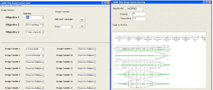
[image:20.595.68.528.71.287.2]

(21)

[image:21.595.157.450.83.265.2]

Fig. 6. Work flow between the Optimisation System and third party software NAPA

[image:21.595.83.519.411.470.2]

The vessel is modelled in NAPA (Fig. 7) and can be modified for each design experiment (or design layout) with respect to each optimisation parameter via NAPA macro. For each design experiment, the relevant adjustments of Draught and Displacement are made during the optimisation process (Fig. 8).

Fig. 7. Ship model built in NAPA for optimization.

[image:21.595.72.506.525.709.2]

(22)

5.2 Result and Analysis

The calculations are performed using both NSGAII and HCPSO, and the results are compared in terms of the numerical value of objectives and the computing time that each approach takes.

This optimisation has three objectives to maximize, thus three sub-swarms are set. The population size is 30 and the generation is 100. Therefore every sub-swarm has 10 particles. and are set to 2.0.

1

c

2

ω

is gradually decreased from 1.0 to 0.4. Vmax is set to the bounds of decision variable ranges.

χ

is 0.72. The ε-disturbance has 3 steps. The NSGA II uses the parameters setting of prior research

in the same environment [49]. The HCPSO and NSGAII parameters are listed in Table 9.

Table 9

The setting of the parameters in the case study for HCPSO and NSGAII

HCPSO Parameters’ Setting NSGAII Parameters’ Setting

Parameters Name Parameters Value Parameters Name Parameters Value Constriction Function 0.72 SBX (Simulated binary crossover) 10 Inertia weight 1.0 to 0.4 polynomial mutation 20 Cognitive parameter 2 crossover probabilities 0.9

Social parameter 2 mutation probabilities 0.1

Population 30 Population 30

Generation 100 Generation 100

The optimisation is performed using a PC (Dual Core 2.4GHz, 3 GB RAM) environment and takes 80h (Fig. 9). At the end of this run, 2625 different designs are obtained in design space, with 615 of them being unfeasible designs. Therefore 2010 (=2625-615) feasible designs are filtered in design space to obtain only the designs that belong to the Pareto front.

The selected HCPSO optimisation

solutions are listed in Table 10 together with the NSGAII optimisation. The

comparison of the original design and the selected design

in amidships is also given in Fig. 10.

In this solution (Table 10), the Hs in HCPSO is improved by more than 0.55 m compared to the original design, while the number of car lanes is increased by 6 extra lanes, which is equivalent to an increase of above 50%. The KG limiting value is also increased significantly (0.9 m) thus provides flexibility for future modifications on the basis of changing passenger demands as well as improvement in survivability. When comparing the two optimisation methods, the HCPSO design improves both the limiting KG and significant wave height (Hs) by 0.1m, compared to the NSGAII design. Both methods provide the same solution for the cargo capacity by increasing the lower-hold height and car deck height, thus yielding more cargo capacity.

[image:22.595.71.533.300.422.2]

(23)

means the HCPSO takes 35% less time in looking for Pareto solutions compared to NSGAII. In a more complex environment, such as a real ship application with many objectives, this provides an advantage in terms of completing the design faster and thus cheaper.

(a) (b)

[image:23.595.76.506.139.523.2]

(c) (d)

Fig. 9. Optimisation results of HCPSO; (a) Limiting KG vs Hs; (b) Cargo Capacity vs Limiting KG; (c) Cargo Capacity vs Hs (d) 3D optimization feasible designs

All feasible results are given in Fig. 8. The relationships between different variables are

shown for designers to make a direct observation and to select the appropriate solution

according to their practical preference. All of the feasible designs are listed in 3D space (Fig.

9 d).

Table 10

Comparison of the

original design and selected designs which are optimal solutions for HCPSO and NSGAII

No Optimisation Variables Original Design NSGAII Design HCPSO design

(24)

2 Lower-hold height (from car deck) 2.6m 5.2m 5.2m

3 Side Casing width (m) No side-casing 1m 1m

Watertight transverse bulkheads (In frame numbers)

4 Transverse Bulkhead 02 27 27 27

Optimisation Objectives

1 HS value (m) 4.641 5.082 5.179

2 KG limiting value (m) 14.012 14.813 14.9085

3 Cargo capacity value (lanes) 8 14 14

[image:24.595.73.503.70.625.2]

(a)Original design (b) selected design Fig. 10. Comparison between original design and selected design based on HCPSO. 6. Conclusions

(25)

With regards to the real ship design case, the internal subdivision optimisation of a ROPAX vessel, with three conflicting objectives (survivability, damage stability and cargo capacity), is carried out. For the search platform, a JAVA based optimisation system and NAPA have been integrated into a multi-agent search framework.

The proposed algorithm provides an improved design, compared to the original design, in every chosen objective with a significant margin, and demonstrates the value of HCPSO. In this design case, the HCPSO displays a better performance both in speed and final results compared to NSGAII. The co-evolution method used in HCPSO provides a good basis for distributed calculation and allows sub-swarm being updated dynamically. The proposed algorithm is structured via a multi-agent system and every agent works remarkably well. It can be concluded that the proposed approach has shown great potential and can be applied to similar and even more complex optimisation problems in ship design, as well as to related areas within the maritime industry.

REFERENCES

[1] Lee D. Multiobjective design of a marine vehicle with aid of design knowledge. International journal for numerical methods in engineering 1997;40:2665-2677；

[2] Thomas M. A pareto frontier for full stern submarines via genetic algorithm. PhD thesis, Ocean Engineering Department, Massachusetts Institute of Technology, Cambridge, Massachusetts, USA, June 1998.

[3] Thomas M. Multi-species pareto frontiers in preliminary submarine design. Foundations of Computing and Decision Sciences 2000；25(4):273–289；

[4] Brown A and Thomas M. Reengineering the naval ship design process. In Proceedings of From Research to Reality in Ship Systems Engineering Symposium, University of Essex, United Kingdom, 1998;

[5] Brown A and Salcedo J. Multiple-Objective optimisation in naval ship design. Naval Engineers Journal 2003;115:4:49-61;

[6] Brown A and Mierzwicki T. Risk metric for multi-objective design of naval ships. Naval Engineers Journal 2004;116: 2: 55-72;

[7] Todd D and Sen P. A multiple criteria genetic algorithm for containership Loading. Proceedings of the Seventh International Conference on Genetic Algorithms, 1997:674–681.

[8] Todd D and Sen P. Multiple criteria scheduling using genetic algorithms in a shipyard environment. In Proceedings of the 9th International Conference on Computer Applications in Shipbuilding, Yokohama, 1997;

[9] Todd D and Sen P. Tackling complex job shop problems using operation based scheduling. The Integration of Evolutionary and Adaptive Computing Technologies with Product/System Design and Realisation, Plymouth, 1998;

[10] Peri D and Campana E. Multidisciplinary design optimisation of a naval surface combatant. Journal of Ship Research 2003; 47:1:1–12;

(26)

in simulation-based design. Journal of Ship Research 2005, 49:3:159–175;

[12] Ölçer A. A hybrid approach for multi-objective combinatorial optimisation problems in ship design and shipping. Computers & OR 2008；35(9): 2760-2775

[13] Boulougouris E and Papanikolaou A. Multi-objective optimisation of a float LNG terminal. Ocean engineering 2008; 35:787-811;

[14] Kennedy J, Eberhart Rc, Particle swarm optimisation. In: Proc. of the IEEE Conf. on Neural Networks, Perth, 1995;

[15] Moore J and Chapman R. Application of particle swarm to multiobjective optimisation, Department of Computer Science and Software Engineering, Auburn University. 1999;

[16] Campana, E.F., Fasano, G.,Peri, D., and Pinto, A. Particle swarm optimisation: Efficient globally convergent modifications. Proceedings of the III European Conference on Computational Mechanics, Solids, Structures and Coupled Problems in Engineering, Lisbon, Portugal,2006;

[17] Pinto A, Peri D and Campana E. Multiobjective optimisation of a containership using deterministic Particle Swarm Optimisation, Journal of Ship Research, 2007:51:3: 217–228;

[18] Mistree F, Smith W, Bras B, Allen J and Muster A, Decision-Based Design: A Contemporary Paradigm for Ship Design. Transactions of SNAME 1990；98：565-597;

[19 ] Margarita R and Coello C. Multi-Objective Particle Swarm Optimizers: A Survey of the State-of-the-Art, International Journal of Computational Intelligence Research, 2006; 2:287–308. [20] Parsopoulos K and Vrahatis M, Particle swarm optimisation method in multiobjective problems. In Proceedings of the 2002 ACM Symposium on Applied Computing (SAC’2002), 603–607.

[21] Baumgartner U, Magele CH, and Pareto W, optimality and particle swarm optimisation. IEEE Transactions on Magnetics 2004; 40(2):1172–1175.

[22] Jin Y, Olhofer M and Sendhoff B. Dynamic Weighted Aggregation for Evolutionary Multi-Objective Optimisation: Why Does it Work and How?, Proceedings of the Genetic and Evolutionary Computation Conference, San Francisco, 2001

[23] Hu X And Eberhart R, Multiobjective optimisation using dynamic neighborhood particle swarm optimisation. In Congress on Evolutionary Computation (CEC’2002), 2002;2: 1677–1681.

[24] Parsopoulos K, Tasoulis D, and Vrahatis M, Multiobjective optimisation using parallel vector evaluated particle swarm optimisation, In Proceedings of the IASTED International Conference on Artificial Intelligence and Applications (AIA 2004) 2004;2:823–828.

[25] Chow C and Tsui H. Autonomous agent response(2004) learning by a multi-species particle swarm optimisation, In Congress on Evolutionary Computation (CEC’2004) 2004; 1:778–785.

[26] Zheng W, LIU Hong, A Cooperative Co-evolutionary and ε-Dominance Based MOPSO, Journal of Software 2007; 18:109−119.

[27] Moore J and Chapman R, Application of particle swarm to multiobjective optimisation, Department of Computer Science and Software Engineering, Auburn University, 1999

[28] Ray T and Liew K A swarm metaphor for multiobjective design optimisation, Engineering Optimisation. 2002; 34(2):141–153.

[29] Fieldsend J and Singh S, (2002), A multiobjective algorithm based upon particle swarm optimisation, an efficient data structure and turbulence, In Proceedings of the 2002 U.K. Workshop on Computational Intelligence, Birmingham, 2002;

(27)

optimisation, In Congress on Evolutionary Computation (CEC’2002), 2002; 2:1051– 1056.

[31] Coello C, PulidoG and Lechuga M. Handling multiple objectives with particle swarm optimisation. IEEE Transactions on Evolutionary Computation, 2004:8:3:256-279.

[32] Li. X A non-dominated sorting particle swarm optimizer for multiobjective optimisation, In Proceedings of the Genetic and Evolutionary Computation Conference (GECCO’2003), Springer. Lecture Notes in Computer Science 2003;2723;37–48;

[33] Sefrioui M and Periaux J, Nash Genetic Algorithms : examples and applications In proceeding of the congress on evolutionary computation 2000: 509-516;

[34] Holt C and Roth A, The Nash equilibrium: A perspective, PNAS 2004; 101: 12: 3999–4002; [35] Deb K, Multi-objective optimisation using evolutionary algorithms, JOHN WILEY & SONS Ltd, 2001.

[36] Zitzler E., Deb K., and Thiele L.. Comparison of Multiobjective Evolutionary Algorithms: Empirical Results. Evolutionary Computation, , 2000,8(2):173—195;

[37] Deb K., Thiele L., Laumanns M., Zitzler E., Scalable Test Problems for Evolutionary Multi-Objective Optimisation, Computer Engineering and Networks Laboratory (TIK), Swiss Federal Institute of Technology, 2001;

[38] Parsopoulos K and Vrahatis M. Recent approaches to global optimisation problems through Particle Swarm Optimisation, Natural Computing2002;1: 235–306;

[39] Shi Yuhui, Eberhart R. Empirical study of particle swarm optimization, Proc of the Congress on Evolutionary Computation, 1999; 1945-1950.

[40] Eberhart R. Shi Yuhui. Comparing inertia weights and constriction factors in particle swarm optimization, Evolutionary Computation, 2000, Proceedings of the 2000 Congress on, Vol. 1 (2000), 84-88

[41] Clerc M., Kennedy J., "The Particle Swarm-Explosion, Stability, and Convergence in a Multidimensional Complex Space", IEEE Transactions on Evolutionary Computation, 2002, vol. 6, p. 58-73;

[42] Trelea, I. C. The particle swarm optimisation algorithm: convergence analysis and parameter selection. Information Processing Letters, 2003, 85(6):317-325.

[43] Turkmen B. A multi-agent system based conceptual ship design decision support system, PhD thesis. Department of Naval Architecture and Marine Engineering, Universities of Glasgow and Strathclyde, 2005;

[44] IMO, SLF 40/INF.14 (Annex 1), (1996), Ro–Ro passenger ship safety: guidance notes on Annex 3 of the agreement concerning specific stability requirements for Ro–Ro passenger ships undertaking regular scheduled international voyages between or to or from designated ports in north west Europe and the Baltic sea.

[45] Sen P and Gerigk M. Some aspects of a knowledge-based expert system for preliminary ship subdivision design for safety, International Symposium PRADS’92 1992;2:1187–1197.

[46] Zaraphonitis G, Boulougouris E and Papanikolaou A. An integrated optimisation procedure for the design of RO-RO passenger ships of enhanced safety and efficiency, proceedings of the 8th international marine design conference, 2003:313-324.

[47] Ölçer A, Tuzcu C, Turan O, Internal hull subdivision optimisation of Ro–Ro vessels in multiple criteria decision making environment, in: Proceedings of the 8th International Marine Design Conference, 2003;1: 339–351.

(28)

multi-attributive group decision-making technique for subdivision arrangement of Ro-Ro vessels. Applied Soft Computing 2006; 6: 221-243.

[49] Turan O, Turkmen B, Tuzcu C, Case-based reasoning approach to internal hull subdivision design, (2004), 4th International Conference on Advanced Engineering Design, 2004, Glasgow.

[50] Turkmen S, Turan O. A new integrated multi-objective optimisation algorithm and its

application to ship design, ship and offshore structures 2007; 2:1: 21 – 37.

[51] Vassalos D, Pawlowski M, Turan O, A Theoretical Investigation on the Capsizal Resistance of Passenger/Ro–Ro Vessels and Proposal of Survival Criteria, Final Report, Task 5, The North West European R&D Project, 1996.