ANALYTICAL MODELLING AND VIBRATION ANALYSIS OF PARTIALLY CRACKED RECTANGULAR
PLATES WITH DIFFERENT BOUNDARY CONDITIONS AND LOADING
Asif Israr 1
, Matthew P. Cartmell 1
, Emil Manoach 2
, Irina Trendafilova 3
, Wiesław Ostachowicz 4
, Marek Krawczuk
5
, and Arkadiusz śak 6
1
Department of Mechanical Engineering, James Watt South Building, University of Glasgow, Glasgow, G12 8QQ, Scotland, UK. email: [email protected], [email protected]
2
Institute of Mechanics, Bulgarian Academy of Sciences, Acad. G. Bontchev Str., Block4,1113 Sofia, Bulgaria. email: [email protected]
3
Department of Mechanical Engineering, University of Strathclyde, 75 Montrose Str., Glasgow, G1 1XJ, Scotland, UK. email: [email protected]
4
Institute of Fluid Flow Machinery, Polish Academy of Sciences, ul. Gen Fiszera 14, 80-952, Gdańsk, & Gdynia Maritime University, Faculty of Navigation, Al. Jana Pawla II, 81-345 Gdynia, Poland.
email: [email protected]
5
Institute of Fluid Flow Machinery, Polish Academy of Sciences, ul. Gen Fiszera 14, 80-952, Gdańsk, & Technical University of Gdańsk, Department of Electric and Control Engineering, Narutowicza 11/12, 80-952 Gdańsk, Poland.
email: [email protected]
6
Institute of Fluid Flow Machinery, Polish Academy of Sciences, ul. Gen Fiszera 14, 80-952, Gdańsk. email: [email protected]
Abstract
This study proposes an analytical model for vibrations in a cracked rectangular plate as one of the results from a programme of research on vibration based damage detection in aircraft panel structures. This particular work considers an isotropic plate, typically made of aluminium, and containing a crack in the form of a continuous line with its centre located at the centre of the plate, and parallel to one edge of the plate. The plate is subjected to a point load on its surface for three different possible boundary conditions, and one examined in detail. Galerkin’s method is applied to reformulate the governing equation of the cracked plate into time dependent modal coordinates. Nonlinearity is introduced by appropriate formulations introduced by applying Berger’s method. An approximate solution technique, the method of multiple scales, is applied to solve the nonlinear equation of the cracked plate. Results are presented in terms of natural frequency versus crack length and plate thickness, and the nonlinear amplitude response of the plate is calculated for one set of boundary conditions and three different load locations, over a practical range of external excitation frequencies.
Overview
Thin plate structures have gained special importance and notably increased application in recent years. Complex structures such as aircraft, ships, steel bridges, sea platforms etc., all use metal plates. For example, it has been observed that plate panels on the tips of aircraft wings are mainly under transverse pressure, and are often subjected to normal and shear forces which act in the plane of the plate. The plate may not behave as intended if it contains even a small crack or form of damage, and such small disturbances can then create a complete loss of equilibrium and cause failure.
The literature has been reviewed for research on cracked plates under tension and bending. Khadem and Rezaee [1] introduced a new technique for vibration analysis of cracked plates and considered the effect of compliance due to bending
concluded from their results that the presence of a crack at a specific depth and depending upon its location, would affect each of the natural frequencies differently. Krawczuk et al. [4] applied a versatile numerical approach for the analysis of wave propagation and damage detection within cracked plates. Wu and Shih [5] theoretically analyzed the dynamic instability and nonlinear response of cracked plates subjected to periodic in-plane load. The results indicated that the stability behaviour and the response of the system are governed by the crack location of the plate, the aspect ratio of the plate, conditions of in-plane loading and the amplitude of vibration. Moreover, increasing the crack ratio i.e. the ratio of the crack length to the length of the edge parallel to the crack, and/or the static component of the in-plane load decreases the natural frequency of the system. Irwin [6] examined a part-through crack in a plate subjected to tension and derived a relation for the crack stress-field parameter and the crack extension force at the boundaries of a flat elliptical crack. Rice and Levy [7] employed two dimensional generalised plane stresses and used Kirchhoff’s plate bending theories with a continuously distributed line-spring to represent a part-through crack, and choose compliance coefficients to match those of an edge-cracked strip in plane strain. The line of discontinuity was of length 2a and the plate was subjected to remote uniform stretching and bending loads along the far sides of the plate. These authors computed the force and moment across the cracked section to determine the stress intensity factor, and the solution to the problem was characterised in terms of the Airy stress function. Their results showed that Krs Krs (where
rs
K is the stress intensity factor for an all-over crack, and Krs is the stress intensity factor of an edge crack in plane strain for the same relative depth lo h, and for remote tensile or bending load) approaches unity with an increase in the ratio of crack length to plate thickness 2a h. Furthermore, at small values of relative depth lo h, the relative changes of stress intensity factors approaches unity for small values of 2a h.
The solutions obtained based on linear models are considered adequate for many practical and engineering purposes although it is recognized that linearized equations usually provide no more than a first approximation. Linearized models of vibrating systems are inadequate in cases where displacements are not small. In addition, problems treated by nonlinear theory exhibit new phenomena for example, the dependence of frequency of vibration on amplitude that cannot be predicted by means of linear theories. Moreover, an example of such a source of nonlinearity is a crack within a plate, which can lead to profound changes in the vibrational response of the system. In this study, much previous work has been considered together, leading to a proposal for a new analytical model for the vibration analysis of a cracked plate. In [8] the authors developed an approximate analytical solution for damage detection in an aircraft panel structure modelled as a cracked isotropic plate without the application of a load, essentially for free vibration. The literature does not appear to contain any substantial references to analytical models for cracked plates undergoing forced vibration. The work presented here considers classical plate theory and includes an arbitrarily located crack within a rectangular plate.
The crack consists of a continuous line and certain simplifying assumptions are made in order to get an initial tractable solution to the vibration problem. Principally, the effects of rotary inertia and through-thickness shear stress effects are neglected. Berger’s formulation is used to generate the nonlinear term within the model differential equation of motion. An approximate analytical solution of the equation for the vibration in the cracked plate for given boundary conditions, is found by the method of multiple scales, followed by the presentation of some numerical results and conclusions.
Governing Equation of the Rectangular Plate and Crack Term
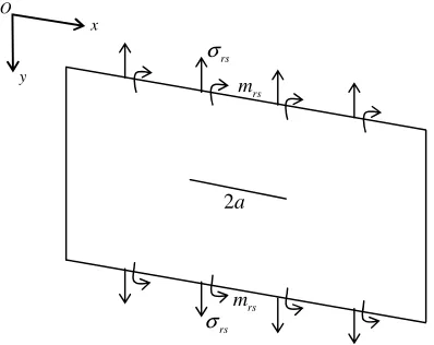
The classical form of the governing equation of rectangular plate is rigorously treated in [9-11]. Here, the equilibrium principle is followed for the derivation of the governing equation of the cracked rectangular plate, in which a crack is present at the centre and parallel to the x-direction of the plate, as depicted in Fig. 1, and consisting of a continuous line of length 2a. The following basic assumptions are summarized:
1. The plate is made of a perfectly elastic, homogeneous, isotropic material and has a uniform thickness h which is considered small in comparison with its other dimensions. 2. All strain components are small enough to allow Hooke’s
law to hold.
3. The normal stress component in the direction transverse to the plate surface is small compared with other stress components, and is neglected in the stress-strain relationship.
4. Shear deformation is neglected in this case and it is assumed that sections taken normal to the middle surface before deformation remain plane and normal to the deflected middle surface of the plate.
5. The effect of the rotary inertia, shear forces and in-plane force in the y-direction i.e. nyand nxy are neglected to make the problem more tractable.
Based upon these assumptions, the final version of the governing equation of the cracked plate takes the following form,
2
4 4 4 2 2 2
4 2 2 2 4 ρ 2 2 2 2 .
∂ ∂ ∂ ∂ ∂ ∂ ∂
+ + = − + + + +
∂ ∂ ∂ ∂ ∂ ∂ ∂ ∂
y
x y z
M
w w w w w w
D h n n P
x x y y t x y y
(1) where D=Eh3 12(1−υ2),
z
P is the load per unit area acting at the surface, ρ is the density of the plate, nx is the in-plane or membrane force, My, and ny are the moment and in-plane force per unit length due to inclusion of crack at the centre of the plate, respectively.
these crack terms is obtained from the Rice and Levy [7] model (in Eqs. (10) and (11)). The Rice and Levy approach is based on Kirchoff’s bending theory for thin plates, and the assumptions involved in this theory lead to important simplifications in the governing equations. Actually, the results are presented for the stress intensity factors in part-through cracked plates, provided that the crack is not too deep. These stress relationship are used and then by making use of Eqs. (8) and (9), a new relationship for the force and moment caused by the crack has been developed, which is dealt in the following section.
Later, Pz in Eq. (1) is replaced by a point load Pz based on the application of the appropriate delta function in Eq. (24) to make it compatible with the experimental configuration. Furthermore, in practice, it is straightforward to implement this type of loading.
Crack Terms Formulation
Rice and Levy [7] obtained an approximate relation for nominal tensile and bending stresses at the location of the crack. These two relations are taken after some rearrangement, and making use of the relationships within Eqs. (8) and (9) from which it can be deduced that mrs=6σrs. A representation of these stresses is given in Fig. 1.
Fig. 1 Line Spring model representing the bending and tensile stresses for a part-through crack of length 2a, after [7]
(
)
22
,
6 (1 ) 2
rs o o rs
tb tt
a
h a
σ σ
α α υ
=
+ − + (2)
and,
2
.
3 (3 )(1 ) 2
6
rs o rs
o bt
bb
a
m m
h a α
α υ υ
=
+ + − +
(3)
We define σrsand mrsas the nominal tensile and bending stresses respectively, at the crack location and on the surface of the plate, σrsand mrsare the nominal tensile and bending
stresses at the far sides of the plate, h is the thickness of the plate, a is the half-crack length, and o
bb α , o
tt
α , o o bt tb α =α are the non-dimensional bending compliance, stretching compliance and stretching-bending compliance coefficients at the crack centre respectively.
This shows that the nominal tensile and bending stresses at the crack location can be regarded as a function of the nominal tensile and bending stresses at the far side of the plate. It is worth noting that Okamura et al. [2] and Khadem and Rezaee [3] also restricted their analysis to the effects of bending compliance. These three compliance coefficients depend upon the crack depth d to plate thickness h and vanish when
0
d= . It is shown in [7] that in general the compliance coefficient is a function of the ratio of crack depth to plate thickness. After suitable nondimensionalisation the compliance coefficients at the centre of the crack takes this form,
1.1547 ,
o
λµ λµ
α = α (4)
where λ µ, =b t, are intermediate variables used in [7] for algebraic simplification. The appropriate compliance coefficients, αλµ, may then be calculated from the following relation, noting that they are valid only for ζ =d h values within the range 0.1-0.7. In the present analysis, we take ζ =0.6, leading to calculation of the compliance coefficients [1-2, 7] as follows,
1 2 3 4
2
5 6 7 8
1.98 0.54 18.65 33.70 99.26 , 211.90 436.84 460.48 289.98
tt
ζ ζ ζ ζ
α ζ
ζ ζ ζ ζ
− + − +
=
− + − +
(5)
1 2 3 4
2
5 6 7 8
1.98 3.28 14.43 31.26 63.56 , 103.36 147.52 127.69 61.50
bb
ζ ζ ζ ζ
α ζ
ζ ζ ζ ζ
− + − +
=
− + − +
(6)
1 2 3 4
2
5 6 7 8
1.98 1.91 16.01 34.84 83.93 . 153.65 256.72 244.67 133.55
bt tb
ζ ζ ζ ζ
α α ζ
ζ ζ ζ ζ
− + − +
= =
− + − +
(7) This means that uniformly distributed tensile and bending stresses are at the two sides of the crack location, and these tensile and bending stresses can be expressed in term of tensile and bending force effects. Therefore, we can write the tensile and bending stresses at the far sides as [7],
/ 2
/ 2 1
( , , ) ,
h rs
rs rs
h
n
x y z dz h h
σ τ
+
−
= =
∫
(8)O
x
y
rs
σ
rs
σ 2a
rs
m
rs
[image:3.595.55.254.388.546.2]/ 2
2 2
/ 2
6 6
( , , ) ,
h
rs rs rs
h
m M z x y z dz
h h τ
+
−
= =
∫
(9)where r s, =1, 2 are intermediate variables required for algebraic simplification. nrsand Mrsare the force and moment per unit length in the y-direction at the far sides of the plate, respectively, and τrs( , , )x y z is the stress state.
The force and moment were calculated from two-dimensional plane stress-plate bending theory, with the cracked section represented as a continuous line spring having its compliance matched to that of the edge cracked strip in plane strain. Accordingly, we can write Eqs. (2) and (3) in the form of force and moment as,
(
)
22
,
6 (1 ) 2
rs o o rs
tb tt
a
n n
h a
α α υ
=
+ − +
(10)
and,
2
,
3 (3 )(1 ) 2
6
rs o rs
o bt
bb
a
M M
h a α
α υ υ
=
+ + − +
(11)
where nrs and Mrsare the force and moment per unit length in the y-direction at the crack location of the plate, respectively.
It is evident from the work of Rice and Levy [7] that when two forces are acting on the plate element to stretch and bend it, the results of their work show that the Airy stress function satisfies the compatibility condition in a region where the body force field is zero. Here, it is very useful to mention that the present theory and the model of the Rice and Levy are based on classical plate theory, therefore the force and moment obtained from Eqs (10) and (11) are the required terms and are added into the cracked plate model with a negative sign because damage causes a reduction in the overall stiffness of the plate structure, a phenomenon which can also be seen in the literature, such as the work of Khadem and Razaee [1,3], and Wu and Shih [5]. Therefore, we can write,
(
)
22
, 6α α (1 υ ) 2
≡ − = −
+ − +
y rs o o rs
tb tt
a
n n n
h a
(12)
and,
2
3 (3 )(1 ) 2
6 α
α υ υ
≡ − = −
+ + − +
y rs o rs
o bt
bb
a
M M M
h a (13)
Substituting the values of ny and Myfrom Eqs. (12) and (13) into the Eq. (1), so the governing equation of the plate with crack extends to the following form,
(
)
4 4 4 2 2
4 2 2 4 2 2
2 2
2 2 2
2 2
3 (3 )(1 ) 2
6 2
.
6 (1 ) 2
ρ
α
α υ υ
α α υ
∂ ∂ ∂ ∂ ∂
+ + = − + +
∂ ∂ ∂ ∂ ∂ ∂
∂ −
∂
+ + − +
∂ −
∂
+ − +
x z
rs o
o bt
bb
rs
o o
tb tt
w w w w w
D h n P
x x y y t x
M a
y h a
a w
n y h a
(14)
As the bending stresses at the far sides of the plate are defined by,
2 2
2 2 ,
rs
w w
M D
y υ x
∂ ∂
= − +
∂ ∂
(15)
then Eq. (15) can be substituted into Eq. (14) to get the final form,
(
)
4 4 4 2 2
4 2 2 4 2 2
4 4
4 2 2
2 2 2
2
2
3 (3 )(1 ) 2
6 2
.
6 (1 ) 2
ρ
υ α
α υ υ
α α υ
∂ ∂ ∂ ∂ ∂
+ + = − + +
∂ ∂ ∂ ∂ ∂ ∂
∂ ∂
+ +
∂ ∂ ∂
+ + − +
∂ −
∂
+ − +
x z
o o bt
bb
rs
o o
tb tt
w w w w w
D h n P
x x y y t x
a w w
D
y y x
h a
a w
n y h a
(16)
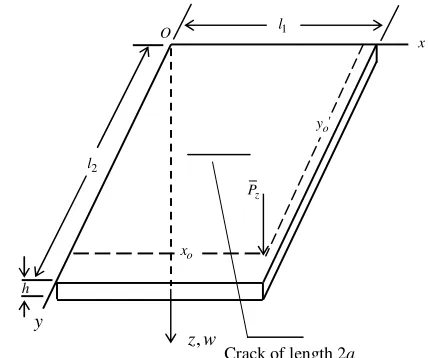
General Solution for a Vibrating Cracked Plate Now we consider the rectangular plate of Fig. 2, of length 1
l in the x-direction and l2 in the y-direction containing a crack which consists of a continuous line of length 2a located at the centre and parallel to the x-direction of the plate.
Fig. 2 Isotropic Plate loaded by concentrated force and
small crack of length 2a at the centre, and parallel to the
x -axis
y
, z w
O
z
P
x
2 l
1 l
o
x
o
y
[image:4.595.310.524.513.692.2]A point load Pz based on the application of the appropriate delta function (in Eq. (24)) is introduced at the location of
(x yo, o).
Leissa [9] studied a wide range of rectangular plates with different boundary conditions, producing seminal data on natural frequencies and mode shapes. Many approaches have been adopted from time to time to form the general solution for vibrating plate. Yagiz and Sakman [12] observed the dynamic response of a bridge modelled as an isotropic plate under the effect of a moving load with all sides simply supported. They considered a vehicle in the form of a seven degree of freedom system as the moving load. A mathematical model was obtained by the use of Lagrange’s formulation and was used to investigate the dynamic response of the bridge and vehicle. Au and Wang [13] studied the dynamic responses in terms of sound radiation from forced vibration of an orthotropic plate with the effects of moving mass, damping coefficient, boundary conditions. Fan [14] analyzed the transient vibration and sound radiation of a rectangular plate with visco-elastic boundary supports subjected to impact loading and obtained the sound radiation pressure in the time and frequency domain by the Rayleigh integral. Mukhopadhyay [15] presented a numerical method for the solution of rectangular plates having different edge conditions and loadings. Young [16] investigated and calculated the set of functions, which define the normal modes of vibration of a uniform beam and obtained the solution for the plate problem with different boundary conditions by the use of Ritz method. Stanišië [17] and Nagaraja and Rao [18] obtained an
approximate solution to find the dynamical behaviour of rectangular plates for different boundary conditions.
The solution for the governing differential equation of the plate subjected to transverse loading is obtained by defining the characteristic functions depending upon the boundary conditions of the plate. The basic model for solution is the one in which all edges are simply supported, while for other boundary conditions the principle of superposition holds [11,19]. The most general form of the transverse deflection of the plate is
1 1
( , , ) mn m n mn( ),
n m
w x y t ∞ ∞ A X Yψ t
= =
=
∑ ∑
(17)whereXmand Ynare the characteristic or modal functions of the cracked rectangular plate,Amnis an, as yet, arbitrary amplitude and ψmn( )t is the time dependent modal coordinate. The appropriate expressions for the characteristic or modal functions are given below and satisfy the stated boundary conditions of the plate. For all cases l1and l2are the lengths of the sides of the plate along the x and y directions respectively. Three boundary condition cases are given next.
Boundary Condition 1. Two adjacent edges are clamped while the other two edges are free – CCFF [9,16,18,19]
1 1 1 1
cos m cosh m sin m sinh m ,
m m
x x x x
X
l l l l
λ λ λ λ
γ
= − − −
(18)
2 2 2 2
cos n cosh n sin n sinh n .
n n
y y y y
Y
l l l l
λ λ λ λ
γ
= − − −
(19) The λm n, and the γm n, are mode shape constants and can be found in standard reference text such as [9,19].
Boundary Condition 2. Two adjacent edges are clamped while the other two edges are freely supported – CCSS [20]
1 1
1 1 1 1
1 3
sin sin cos cos ,
2 2 2 2
m m m
m x m x m x m x
X
l l l l
π π π π
∞ ∞
= =
= = −
∑
∑
(20)
1 1
2 2 2 2
1 3
sin sin cos cos .
2 2 2 2
n n n
n y n y n y n y
Y
l l l l
π π π π
∞ ∞
= =
= = −
∑
∑
(21) Boundary Condition 3. All sides are simply supported – SSSS [9,10,12]
1 1
sin ,
m m
m x X
l π
∞
=
=
∑
(22)1 2
sin .
n n
n y Y
l π
∞
=
=
∑
(23)
The lateral load Pz at position (xo,yo) can be readily expressed as follows [14]
( ) ( ) ( )
z o o o
P =P t δ x−x δ y−y (24) Substituting the definition of w x y t( , , ) from Eq. (17) and Pz from Eq. (24) into Eq. (16), we get,
(
)
4 4 4 2
4 2 2 4 2
2 2
2 2 2
4 4
4 2 2
( )
2 ( )
2
( ) ( )
6 (1 ) 2 2
3 (3 )(1 ) 2 6
ψ
ψ ρ
ψ ψ
α α υ
υ ψ
α
α υ υ
∂ ∂ ∂ ∂
+ + = −
∂ ∂ ∂ ∂ ∂
∂ ∂
+ −
∂ + − + ∂
∂ ∂
+ +
∂ ∂ ∂
+ + − +
m m n n
n m mn mn m n
m n
x n mn o o rs m mn
tb tt
n m n
m mn
o o bt
bb
X X Y Y t
D Y X A t h A X Y
x x y y t
X a Y
n Y A t n X A t
x h a y
a Y X Y
D X A
y y x
h a
0
( )
( ) (δ ) (δ ).
+ o − − o
t
P t x x y y
(25)
middle surface strains and when the deflection is of the order of magnitude of the thickness of the plate. This can be used to obtain forms for the in-plane forces nx and nrs per unit length in the x and y direction respectively, and applies theory predominantly based on aspect ratios equal to 1, 1.5, 2, and infinity. Berger showed that this approach works well for combinations of simply supported and clamped boundary conditions, as shown previously. We note in passing that Wah [22] and Ramachandran and Reddy [23] also applied Berger’s formulation efficiently for analysing the nonlinear vibrations of undamped rectangular plates.
To make the form of the in-plane forces, the middle surface strains in the x and y directions can be given by [11],
2 1 , 2 x u w x x
ε =∂ + ∂
∂ ∂ (26) 2 1 , 2 y v w y y
ε =∂ + ∂
∂ ∂ (27)
where u and v are the displacements in the x and y directions respectively.
Accordingly, we can write the in-plane forces as, [11],
(
)
2 ,
1
x x y
Eh
n ε υε
υ = + − (28)
(
)
2 . 1rs y x
Eh
n ε υε
υ
= +
− (29)
Substituting Eqs. (26) and (27) into Eqs. (28) and (29), we get 2 2 2 1 1 ,
12 2 2
x
n h u v w w
D x υ y x υ y
∂ ∂ ∂ ∂
= + + +
∂ ∂ ∂ ∂ (30)
and therefore for y,
2 2
2
1 1
.
12 2 2
rs
n h v u w w
D y υ x y υ x
∂ ∂ ∂ ∂
= + + +
∂ ∂ ∂ ∂ (31)
We multiply Eqs. (30) and (31) by dxdy and integrate over the plate area, and then impose the conditions that u and v vanish at the external boundaries and around the crack due to symmetry, leading to,
1 2 2 2
2 1 2 0 0 1 , 12 2 l l x
n h l l w w
dxdy
D x υ y
∂ ∂ = + ∂ ∂
∫∫
(32) and,1 2 2 2
2 1 2 0 0 1 . 12 2 l l rs
n h l l w w
dxdy
D y υ x
∂ ∂ = + ∂ ∂
∫∫
(33)Applying the definition of w x y t( , , ) from Eq. (17) we get, 2 2
1 mn ( )
x mn mn
n =DF A ψ t , (34)
where
1 2 2 2
2 2
1 2 1 1
1 2 0 0
6 , n l l m n mn m n m X Y
F Y X dxdy
x y
h l l υ
∞ ∞ = = ∂ ∂ = + ∂ ∂
∑ ∑ ∫∫
(35)and, 2 2
2 mn ( ),
rs mn mn
n =DF A ψ t (36)
where
1 2 2 2
2 2
2 2 1 1
1 2 0 0
6
. n
l l
n m
mn n m m
Y X
F X Y dxdy
y x
h l l υ
∞ ∞ = = ∂ ∂ = + ∂ ∂
∑ ∑ ∫∫
(37) Substituting the in-plane forces nx and nrs from Eqs. (34) and (36) into Eq. (25), multiplying each part of Eq. (25) by the modal function Xm and Yn for one of the three example boundary conditions mentioned above, and then integrating over the plate area, we find that,3
( ) ( ) ( ) .
mn mn mn mn
M ψɺɺt +K ψ t +G ψ t =P (38) where 1 2 2 2 1 1 0 0 , m n l l
mn n m mn
h
M A X Y dxdy
D
ρ ∞ ∞
= =
=
∑ ∑
∫ ∫
(39)
(
)
1 2 1 1 0 0 2 2 , 3 (3 )(1 ) 26
m n
n
iv iv
n m n m
l l iv
m n m
mn n m mn m n
o o bt
bb
X Y X Y Y X
a X Y Y X
K A X Y dxdy
h a
υ
α
α υ υ
∞ ∞ = = + ′′ ′′+ ′′ ′′ + = − + + − +
∑ ∑
∫ ∫
(40)(
)
1 2 2 1 3 2 2 1 10 0 2
, 2
6α α (1 υ ) 2
∞ ∞ = = − ′′ ′′ = + + − +
∑ ∑
∫ ∫
n mn mmn m m
l l
mn n m mn n n
o o
tb tt F X X Y
G A aF X Y Y dxdy
h a
(41) The integral of the delta function is given by
0
( ) ( ) ( )
m m o
X x δ x x dx X x ∞
−∞
− =
( ) ,
o
mn mn
P t
P Q
D
= (42)
where Qmn =Xm(x0)Y yn( 0). (43) Equation (38) is in the form of the well known Duffing equation containing a cubic nonlinear term, and can be re-stated as
2 3
( ) ( ) ( ) ( ) ,
mn
mn
mn o
t t t P t
D λ
ψɺɺ +ω ψ +β ψ = (44)
where
2 ,
mn
mn mn
K M
ω = (45)
,
mn mn
mn
G M
β = (46)
,
mn mn
mn
Q M
λ = (47)
and ωmn is the natural frequency of the cracked rectangular plate.
Now if it is assumed that the system is under the influence of weak classical linear viscous damping µ, then the equation of the model of the rectangular cracked plate becomes,
2 3
( ) 2 ( ) ( ) ( ) ( ).
mn
mn
mn o
t t t t P t
D λ
ψɺɺ + µψɺ +ω ψ +β ψ = (48)
Letting the load be harmonic, such that, ( ) cos
o mn
P t =p Ω t (49)
leads to,
2 3
( ) 2 ( ) ( ) ( ) cos .
mn
mn
mn mn
t t t t p t
D λ
ψɺɺ + µψɺ +ω ψ +β ψ = Ω (50)
Instead of using the excitation frequency Ωmn as a parameter, we introduce a detuning parameter, σmn, which quantitatively
describes the nearness of Ωmn to ωmn and this is a case of primary resonance. This has the advantage of clarifying identification of the terms in the governing equation at first order perturbation that lead to secular terms. Accordingly we write, [24],
ω εσ
Ωmn = mn+ mn (51)
where ε is an arbitrarily small perturbation parameter.
To obtain a uniformly valid approximate solution to this problem it is necessary to order the cubic term, the damping, and the excitation. To accomplish this we choose to set the following to O(ε)1 ,
, mn mn, p p.
µ=εµ β =εβ =ε (52)
After substituting Eqs. (51) and (52) into Eq. (50), it becomes as follows,
2 3
( ) 2 ( ) ( ) ( ) cos( ) . mn
mn
mn mn mn
t t t t p t
D
λ
ψɺɺ + εµψɺ +ω ψ +εβ ψ =ε ω +εσ
(53) This introduces damping, the cubic nonlinearity, and the excitation to first order perturbation, which is considered to be in line with the appropriate experimental configuration, and other work on weakly nonlinear vibrating systems [24-27]. It is important to note here that for Duffing equations the coefficient of the cubic term, in this case εβmn, can be numerically positive or negative, leading to overhangs of the response curve in the frequency domain to the right or left, respectively.
The Method of Multiple Scales
The method of multiple scales is well discussed in the seminal work of Nayfeh and Mook [24] and also in the well known books of [25], and [26]. Cartmell et al. [27] reviewed the multiple scales method as applied to weakly nonlinear dynamics of mechanical systems. For the method of multiple scales, the solution of the equation is approximated by a uniformly valid expansion of the form,
2
1 1 1
( , ) ( , ) ( , ) ( ),
mn t o mn T To mn T To o
ψ ε =ψ +εψ + ε (54)
where ψomn(T To, 1) and ψ1mn(T To, 1) are functions yet to be determined. Independent time scales are introduced where To is nominally considered as fast time and T1 as slow time, such that, To=t and T1=εt. We can express the excitation in term of To and T1 as
(
1)
( ) cos .
o mn o mn
P t =εp ω T +σ T (55) Substituting the expansion of Eq. (54) and the excitation term from Eq. (55) into Eq. (53), we get,
[
]
[
]
{
}
(
)
1 1
1
2 2 2 2 2 2
1 1 1
2 2 2
1 1 1
2 2 2 2 3 3 2
1
1
2 2
( ) 2 2 2 ( )
( ) ( )
cos .
o o
mn mn mn
o mn mn
o o mn o mn
o o mn o mn
o mn mn mn
mn
mn o mn
D D D D D D D D
o D D D D o
o o
p T T
D
ε ε ψ ε ε ε ψ
ε εµ ε ψ ε µ ε ψ εµ ε
ω ψ εω ψ ω ε εβ ψ εψ ε
λ
ε ω σ
+ + + + +
+ + + + + +
+ + + + + +
= +
(56) Separating terms of like order ε yields, to order εo:
2 2
0,
o o mn mn o mn
Dψ +ω ψ = (57)
and to order ε1:
(
)
2 2 3
1 1 1
1
2 2
cos .
mn
o mn mn o o mn o o mn mn o mn
mn
mn o mn
D D D D
p T T
D
ψ ω ψ ψ µ ψ β ψ
λ
ω σ
+ = − − −
+ +
(58) The higher orders of ε2, ε3 and so on, may be neglected because higher order perturbation equations will yield negligible corrections for the problem as set up here. The general solution of Eq. (57) can be written as
1 1
( ) i mn oT ( ) i mn oT,
o mn B T e B T e
ω ω
ψ = + −
(59)
where B is an unknown complex amplitude and B is the complex conjugate ofB. This amplitude will be determined by eliminating the secular terms from ψ1mn. Substituting the solution from Eq. (59) into Eq. (58), we get,
{
}
{
}
{
}
(
)
2 2
1 1 1 1 1
1 1
3
1 1 1
2 ( ) ( ) 2 ( ) ( )
( ) ( ) cos ,
mn o mn o
mn o
mn o mn o
mn o mn o
i T i T
mn mn o
i T i T
o
i T i T mn
mn mn o mn
D D D B T e B T e
D B T e B T e
B T e B T e p T T
D
ω ω
ω ω
ω ω
ψ ω ψ
µ
λ
β ω σ
− − − + = − + − + − + + + (60) which, after dropping the argument T1 in the complex amplitudes, leads to the following,
{
}
{
}
(
)
2 2
1 1 1
3 3 3 3 1 2 2 3 cos .
mn o mn o
mn o
mn o mn o
mn o
mn o mn o
mn o
i T i T
mn mn mn mn
i T i T
i T
mn
mn i T i T
i T
mn
mn
mn o mn
D iD Be Be
B e B e Be
i
BB Be Be Ae
p T T
D ω ω ω ω ω ω ω ω
ψ ω ψ ω ω
ω µ β ω λ ω σ − − − − + = − − + − − + + − + + (61) Expressing cos
(
ωmn oT +σmnT1)
in complex form, we get,1
1
2 2
1 1 2
3 3 2 2 3 2 , mn o o mn mn o mn mn i T
mn mn mn mn i T
mn i T
mn
i D B i B
D e
B B pe D B e cc
ω σ
ω
ω µω
ψ ω ψ λ
β β − − + = − + − + (62) where cc denotes the complex conjugate of the preceding terms. Any particular solution of Eq. (62) can have secular terms containing the factor i To
o
T eω unless D B1 =0. To eliminate the secular terms from Eq. (62), we must put,
1
2 1
2 2 3 0.
2
mn
i T
mn
mn mn mn
i D B i B B B pe
D
σ
λ
ω µω β
− − − + = (63)
In solving Eq. (63), it is convenient to write the complex amplitude B in the polar form, 1
2
i
B= beα, (64)
where b and α are real amplitude and phase functions of T1 respectively. Substituting Eq. (64) into Eq. (63), we get,
3
1 1
3 8
[cos( ) sin( )] 0,
2
mn
mn mn mn
mn
mn mn
b i b i b b
p T i T
D
β
ω α ω ω µ
λ
σ α σ α
′− ′− −
+ − + − =
(65)
where the prime denotes the derivative with respect to T1. Now, separating the result into real and imaginary parts, we obtain, 1 sin( ), 2 mn mn mn
b b p T
D λ
µ σ α
ω
′ = − + − (66)
3 1 3 cos( ). 8 2 mn mn mn mn mn b
b p T
D
β λ
α σ α
ω ω
′ = − − (67)
Equations (66) and (67) can be transformed into an autonomous system i.e. one in which T1 does not appear explicitly, by letting, κ=σmnT1−α. (68) Substituting Eq. (68) into Eqs. (66) and (67), we get,
sin , 2
mn mn
b b p
D λ
µ κ
ω
′ = − + (69)
3 3 cos . 8 2 mn mn mn mn mn b
b b p
D
β λ
κ σ κ
ω ω
′ = − + (70)
In the case of steady-state motion b′=κ′≈0, and this corresponds to the singular points of Eqs. (69) and (70); that is, sin , 2 mn mn b p D λ µ κ ω = (71) 3 3 cos . 8 2 mn mn mn mn mn b b p D β λ σ κ ω ω
− + = − (72)
Squaring and adding these equations, we obtain,
2 2
2
2 2 2
a [m] ωm
n
[r
ad
/s
]
It is then possible to rearrange Eq. (73) to give the amplitude of the response b as a function of the detuning parameter
mn
σ and the amplitude of the excitationpoand this is the
frequency-response equation, as follows, 2 2
2 2
2 2 2 3
.
8 4
mn
mn mn
mn mn
b
p b D λ β
σ µ
ω ω
= ± − (74)
Numerical Results and Discussion
In this section the results are presented as functions of frequency, half-crack length and plate thickness. Figure 3 shows the plot of amplitude, b as a function of σmn for given µ and p in the form of a frequency-response curve. Each point on this curve corresponds to a singular point. To draw such a curve, one solves for σmn in terms of b. The material properties of aluminium have been considered for different
cases of half-crack length i.e. E = 7.03 x 10¹⁰ N/m2,
ρ = 2660 kg/m3, ν= 0.33, and damping factor, µ = 0.08 while the geometric values of the plate are l1 = 0.5 m, l2 = 1 m, h = 0.01 m and p = 10 N is the load acting upon the surface of the plate at different points. The effect of changing the position of the load is shown in Fig. 3. The natural frequencies without and with the crack for different boundary conditions and aspect ratios are tabulated in Table 1.
Fig. 3 The amplitude of the response as a function of the detuning parameter [rad/s] and the point load at different locations [m] of the plate element.
It may be seen from Table 1 that the presence of the (shown here as a deliberately large) crack at the centre of the plate significantly influences the natural frequency of the first mode of the plate, in all three cases. In the subsequent section attention will be focused on the case for which two adjacent edges are clamped while the other two edges are free (CCFF), and the results are shown for the first mode only. Although it cannot be easily shown in Fig. 3 due to the necessary scaling of the plot, increasing the half-crack length from 0.05 m to 0.125 m introduces small changes to the degree of nonlinear overhang in the softening direction, with some attendant change in the modal natural frequency. It has also been observed that changing the location of the load on the plate slightly affects the global nonlinearity of the system, as shown in Fig. 3 and evidenced by the increasingly wide nonlinear region as the excitation location moves closer to the unsupported corner.
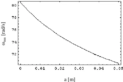
[image:9.595.44.551.87.209.2]
Fig. 4 Plate first mode natural frequency as a function of half-crack length
Figure 4 shows the decrease in the natural frequency as we go on to increase the half-crack length for the same parameters as considered earlier. These changes are very small for small half-crack lengths, as one would expect. Moreover, the natural frequency is also influenced if the geometry of the plate is changed, in particular its length and thickness, in addition to the effect of the half-crack length. Similarly, it may be seen from Fig. 5 that by increasing the thickness of the plate the natural frequency of the first mode also increases for different values of half-crack length. This means that this natural frequency is directly related to the thickness of the plate. The theory presented in this paper currently holds only for a plate
Table 1. Natural frequencies of cracked plate model for different boundary conditions and aspect ratios
Lengths of the sides of the plate
Two adjacent edges clamped, the other two free (CCFF)
Two adjacent edges clamped, the other two simply supported (CCSS)
All edges simply supported (SSSS)
First mode natural frequency, ωmn [rad/s] for a half crack length, a = 0.05 [m]
l1 [m] l2 [m]
un-cracked cracked un-cracked cracked un-cracked cracked 1 1 80.462 70.559 445.666 403.779 77.580 71.119 0.5 1 231.061 227.611 1161.770 1138.530 193.951 189.581 0.5 0.5 321.849 282.237 1782.660 1615.120 310.322 284.475
(xo,yo) = (0.375, 0.375)
- - - (xo,yo) = (0.375, 0.50)
---- (xo,yo) = (0.375, 0.75)
σ
mn [rad/s]
b
[
m
[image:9.595.315.521.438.575.2] [image:9.595.53.271.542.674.2]h [m] ωm
n
[r
ad
/s
]
bN
L
/bL
σ
mn [rad/s]
with a crack at the centre and defined by a continuous line model. Results of this sort could equally be obtained for the cases of CCSS and SSSS, but space limitations currently preclude that.
Fig. 5 Plate first mode natural frequency as a function of the thickness of the plate for the half-crack length 0.05 m
It is also instructive to note that if the cubic nonlinearity
mn
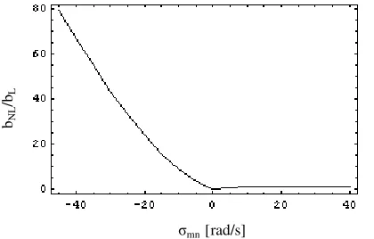
[image:10.595.52.267.135.274.2]β is set to zero then the problem is linearized, but in the case of the nonlinear problem the significant effect of including this term is apparent from the numerical results depicted in Fig. 6. It can be seen in Fig. 6 that the ratio of the nonlinear solution amplitude (whereβmnis set to zero) is very large for negative detuning. This exactly emulates the softening nonlinear characteristic shown in Fig. 4. It can be seen that this ratio reduces close to unity for zero and positive detuning, again fully in line with the softening characteristic observable in Fig. 3. In the Figure bNL is the nonlinear amplitude and bL is the corresponding linear amplitude.
Fig. 6 Comparison between linear and nonlinear model of the cracked rectangular plate
Orientation of the crack at some angle will change the model because there will be more than two components of the crack geometry, one for tensile loading and one for bending along the plate element. Here it is assumed that the crack is parallel to the x-direction of the plate.
Conclusions
This research presents a new analytical model for the vibration analysis of cracked plates subjected to transverse loading at some specified position with different sets of boundary conditions. Berger’s formulation is effectively applied to make the governing equation for vibration of a cracked plate nonlinear and in the form of a Duffing equation. It has been found that for a square plate with the CCFF boundary conditions there is an approximately 12% reduction in natural frequency in the presence of a large centrally located crack of length 0.1 m. However, the reduction in the value of natural frequency is lower for other plate aspect ratios and linear and nonlinear results tend to coalesce for very low amplitude ratios.
Finally, it is concluded that the decrease in the natural frequency when there is a crack present may substantiate use of the model in constructing a vibration based analysis methodology for plate structures and for further development of vibration based health monitoring. Further work is under way to extend the theory of this paper to cracks in arbitrary locations and orientations.
Acknowledgement
This work is part of a larger programme of work that has been carried out under NATO grant CBP.EAP.CLG.981517, and A. Israr’s studentship was kindly provided by the Institute of Space Technology, Pakistan, and the Goudie Bequest of the University of Glasgow, UK.
References
[1] Khadem, S.E. & Rezaee, M., 2000, “Introduction of Modified Comparison Functions for Vibration Analysis of a Rectangular Cracked Plate”, Journal of Sound & Vibration, 236(2), pp. 245-258.
[2] Okamura, H., Liu, H.W., Chu, C. & Liebowitz, H., 1969, “A Cracked Column under Compression, Engineering Fracture Mechanics”, 1, pp. 547-563. [3] Khadem, S.E. & Rezaee, M., 2000, “An Analytical
Approach for Obtaining the Location and Depth of an all-over Part-through Crack on Externally In-plane loaded Rectangular Plate using Vibration Analysis”, Journal of sound and vibration, 230(2), pp. 291-308. [4] Krawczuk, M., Palacz, M. & Ostachowicz, W., 2004,
“Wave Propagation in Plate Structures for Crack Detection”, Finite Elements in Analysis & Design, 40, pp. 991-1004.
[5] Wu, G. Y., & Shih, Y. S., 2005, “Dynamic Instability of Rectangular Plate with an Edge Crack”, Computers and Structures, 84, pp. 1-10.
[6] Irwin, G.R., 1962, “Crack Extension Force for a Part through Crack in a Plate”, Journal of Applied Mechanics, 29, pp. 651-654.
[7] Rice, J.R., & Levy, N., 1972, “The Part through Surface Crack in an Elastic Plate”, Journal of Applied Mechanics, 3, pp. 185-194.
[image:10.595.59.269.472.606.2]Stress and Vibration Analysis VI, P.Keogh, eds., Trans Tech Publications Ltd, Switzerland, 5-6, pp. 315-322 [9] Leissa, A., 1993, Vibration of Plates, NASA SP-160,
National Acoustical and Space Administration, Washington, DC
[10] Szilard, R., 2004, Theories and Applications of Plate Analysis, John Wiley & Sons, USA, pp. 89
[11] Timoshenko, S., 1940, Theory of Plates and Shells, McGraw Hill Book Company, Inc., New York & London
[12] Yagiz, N., & Sakman L. E., 2006, “Vibrations of a Rectangular Bridge as an Isotropic Plate under a Traveling Full Vehicle Model”, Journal of Vibration and Control, 12(1), pp. 83-98.
[13] Au, F.T.K., Wang, M.F., 2005, “Sound Radiation from Forced Vibration of Rectangular Orthotropic Plates under Moving Loads, Journal of Sound and Vibration, 281, pp. 1057-1075.
[14] Fan, Z., 2001, “Transient Vibration and Sound Radiation of a Rectangular Plate with Viscoelastic Boundary Supports”, International Journal for Numerical Methods in Engineering, 51, pp. 619-630. [15] Mukhopadhyay, M., 1979, “A General Solution for
Rectangular Plate Bending”, Forsch. Ing.-Wes., 45, Nr. 4, pp. 111-118.
[16] Young, D., 1950, “Vibration of Rectangular Plates by the Ritz Method”, Journal of Applied Mechanics, 17(4), pp. 448-453.
[17] Stanišië, M.M., 1957, “An Approximate Method
Applied to the Solution of the Problem of Vibrating Rectangular Plates”, Journal of Aeronautical Sciences, 24, pp. 159-160.
[18] Nagaraja, J.V., & Rao, S.S., 1953, “Vibration of Rectangular Plates”, Journal of Aeronautical Sciences, 20, pp. 855-856.
[19] Berthelot, J.M., 1999, Dynamics of Composite Materials and Structures, Institute for Advanced Materials and Mechanics, Springer, New York
[20] Iwato, 1951, “Approximate Calculation for the Frequency of Natural Vibration of a Thin Rectangular Plate the two Adjacent edges of which are Clamped while the other two edges are Freely Supported, Trans JSME, 17(57), 1951, pp. 30-33 (In Japanese)
[21] Berger, H. M., 1955, “A New Approach to the Analysis of Large Deflections of Plates”, Journal of Applied Mechanics, 22, pp. 465-472.
[22] Wah, T., 1964, “The Normal Modes of Vibration of Certain Nonlinear Continuous Systems”, Journal of Applied Mechanics, 31, pp. 139-140.
[23] Ramachandran, J. & Reddy, D.V., 1972, “Nonlinear Vibrations of Rectangular Plates with Cut-outs”, AIAA Journal, 10, pp. 1709-1710.
[24] Nayfeh, A.H. & Mook, D.T., 1979, Nonlinear Oscillations, John Wiley & Sons, Germany.
[25] Kevorkian, J. & Cole, J.D., 1981, Perturbation Methods in Applied Mathematics, Springer-Verlag, 34.
[26] Murdock, J.A., 1999, Perturbations Theory and Methods, SIAM.
[27] Cartmell, M.P., Ziegler, S.W., Khanin, R. & Forehand, D.I.M., 2003, “Multiple Scales Analysis of the