New Periodic Orbits in the Solar Sail restricted three body
problem
J. D. Biggs∗and C. McInnes
Department of Mechanical Engineering, University of Strathclyde, Glasgow, UK
∗E-mail: [email protected]
Thomas Waters
Department of Mathematical Physics, National University of Ireland, Galway, Ireland.
E-mail: [email protected]
In this paper we consider periodic orbits of a solar sail in the Earth-Sun re-stricted three-body problem. In particular, we consider orbits which are high above the ecliptic plane, in contrast to the classical Halo orbits about the collinear equilibria. We begin with the Circular Restricted Three-Body Prob-lem (CRTBP) where periodic orbits about equilibria are naturally present at linear order. Using the method of Lindstedt-Poincar´e, we construct nth or-der approximations to periodic solutions of the nonlinear equations of motion. In the second part of the paper we generalize to the Elliptic Restricted Three-Body Problem (ERTBP). A numerical continuation, with the eccentricity, e, as the varying parameter, is used to find periodic orbits above the ecliptic, start-ing from a known orbit ate= 0 and continuing to the required eccentricity of e= 0.0167. The stability of these periodic orbits is investigated.
Keywords: Periodic orbits, solar sail, elliptic three body problem
1. Introduction
three body problem (ERTBP).
There has been some work already carried out regarding solar sails in
the 3-body problem. McInnes
1first described the surfaces of equilibrium
points. In Baoyin and McInnes,
2the authors describe periodic orbits about
equilibrium points in the solar sail three body problem, however they
con-sider only equilibrium points on the axis joining the primary masses,
cor-responding to artificial Lagrange points (analogous to the classical ‘halo’
orbits
3,4).
In this paper we examine the solutions to the linearised equations of
motion and discuss their stability in the CRTBP. We find that periodic
orbits exist at linear order, and we use these linear solutions to find higher
order approximations to periodic solutions of the non-linear system using
the method of Lindstedt-Poincar´e.
5,6These approximate orbits are then
fine-tuned using a differential corrector to find initial conditions that yield
periodic solutions to the full non-linear model.
5Following this we generalize the problem to the solar sail ERTBP
7in
the Earth-Sun system. A numerical continuation, with the eccentricity
e
as the varying parameter, is used to find periodic orbits above the ecliptic,
starting from a known orbit in the CRTBP (
e
= 0) and continuing to the
required eccentricity
e
= 0
.
0167. The stability of some periodic orbits above
the ecliptic are investigated and it is shown that they are unstable and that
a bifurcation occurs at
e
= 0.
2. Equations of motion in the rotating frame
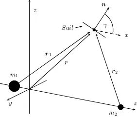
We follow the conventions set out in McInnes.
1We consider a rotating
coor-dinate system in which the primary masses are fixed on the
x
-axis with the
origin at the centre of mass, the
z
-axis is the axis of rotation and the
y
-axis
completes the triad. We choose our units to set the gravitational constant,
the sum of the primary masses, the distance between the primaries, and
the magnitude of the angular velocity of the rotating frame to be unity. We
shall denote by
µ
= 3
×
10
−6the dimensionless mass of the smaller body
m
2, the Earth, and therefore the mass of the larger body
m
1, the Sun, is
given by 1
−
µ
(see Figure 1).
Denoting by
r
,
r
1and
r
2the position of the sail w.r.t. the origin,
m
1and
m
2respectively, the solar sail’s equations of motion in the rotating
frame are
d
2r
dt
2+ 2
ω
×
d
r
dt
=
a
−
ω
×
(
ω
×
r
)
− ∇
V
≡
F
,
(1)
the classical equations of motion in the CR3BP by the radiation pressure
acceleration term
a
=
β
(1
−
µ
)
r
2 1(
b
r
1.
n
)
2n
,
(2)
where
β
is the sail lightness number, and is the ratio of the solar radiation
pressure acceleration to the solar gravitational acceleration. Here
n
is the
unit normal of the sail and describes the sail’s orientation. We define
n
in
terms of two angles
γ
and
φ
w.r.t. the rotating coordinate frame,
n
= (cos(
γ
) cos(
φ
)
,
cos(
γ
) sin(
φ
)
,
sin(
γ
))
,
(3)
where
γ, φ
are the angles the normal makes with the
x
-
y
and
x
-
z
plane
respectively (see Figure 1).
Equilibria are given by the zeroes of
F
in (1). We find a 3-parameter
family of equilibria, as described in McInnes.
1These are found by specifying
the lightness number
β
and the sail angles
γ
and
φ
, and solving
F
= 0.
To simplify facilitate the search for orbits we initially assume
φ
= 0 so the
equilibrium (and sail normal) is in the
x
-
z
plane. In Figure 2 we show some
of the equilibria near the Earth for low
β
values. Practically speaking, while
a
β
value of about 0
.
3
−
0
.
4 is considered within the realm of possibility
of current engineering, to put the analysis in this paper well within the
near-term we will consider very modest
β
values of about 0
.
05.
3. Linearised system
We linearise about the equilibrium point (in the
x
-
z
plane) by making the
transformation
r
→
r
e+
δr
, Taylor expanding
F
about
r
e, and neglectingx z
x y
r1
r2 r
n
γ
m2
m1
[image:3.595.225.366.516.638.2]Sail
0.985 0.99 0.995 1 1.005 1.01 -0.015 -0.01 -0.005 0 0.005 0.01 0.015 b
c bc bc
L1 L2
Earth β= 8 > > > < > > > :
0.03 0.05 0.1 0.2 0.4
xe
[image:4.595.224.369.161.299.2]ze
Fig. 2. Surfaces of equilibrium points in the xe-ze parameter space. Each curve is
specified by a constant value ofβ, and the position of the equilibrium point along the curve is given by γ. The grey shaded regions denote areas where equilibrium is not possible.
the terms quadratic in
δ
r
. We assume the orientation of the sail will remain
fixed under perturbation of the sail position, in which case
γ, φ
and
β
are
constants. Letting
δ
r
= (
δx, δy, δz
)
Tand
X
= (
δ
r
, δ
r
˙
)
T, our linear system
is ˙
X
=
A
X
with
A
=
µ
0
I
M
Ω
,
M
=
a
0
b
0
c
0
d
0
e
,
Ω =
0 2 0
−
2 0 0
0 0 0
,
(4)
where a dot denotes differentiation w.r.t.
t
,
a
= (
∂
xF
x)
|
e,
b
= (
∂
zF
x)
|
e,
c
= (
∂
yF
y)
|
e,
d
= (
∂
xF
z)
|
e,
e
= (
∂
zF
z)
|
e,
and
b
6
=
d
. Here
F
adenotes the
a
-th component of
F
, and
M
is sparse due
to
y
e= 0.
The key difference between this analysis and the classical orbits about
the collinear Lagrange points is the term
d
6
= 0, which appears precisely
because we are linearising about an equilibrium point with
z
e6
= 0. This
means we cannot decouple the
z
-equation.
The characteristic equation of the Jacobian
A
is bi-cubic (whose
cor-responding cubic equation has real roots); this means the eigenvalues of
A
are either in pairs of pure imaginary conjugates or real and of opposite
sign. Thus equilibria in the
x
-
z
plane will have the dynamical structure of
centres and saddles, akin to the classical collinear Lagrange points.
If we label the eigenvectors associated with
λ
ai
(
a
= 1
,
2) as
u
a+
w
ai
,
solution of the linear system (4) is
X
(
t
) = cos(
λ
1t
)
£
A
u
1+
B
w
1¤
+ sin(
λ
1t
)
£
B
u
1−
A
w
1¤
+ cos(
λ
2t
)
£
C
u
2+
D
w
2¤
+ sin(
λ
2t
)
£
D
u
2−
C
w
2¤
+
Ee
λrtv
1
+
F e
−λrtv
2.
(5)
We see that due to the coupling of the
z
-equation in the linear system, which
in turn is due to our choice of
z
e6
= 0, the linear order solution naturally
contains periodic solutions in
both
linear frequencies. By setting
E
=
F
= 0
we may switch off the real modes, and by setting either
A
=
B
= 0 or
C
=
D
= 0 we have periodic solutions in the frequency of our choice.
4. High-order approximations to periodic orbits
The linear solutions given in the previous section will only closely
approx-imate the motion of the sail given in (1) for small amplitudes. For larger
amplitude periodic orbits, we compute high order approximations using
the method of Linstedt-Poincar´e.
5This procedure is well known and is
described in the literature, for example.
3,4We let
ε
be a perturbation parameter and expand each coordinate as
x
→
x
e+
εx
1+
ε
2x
2+
. . .
etc. We rescale the time coordinate
τ
=
ωt
with
ω
= 1 +
εω
1+
. . .
, and group together the powers of
ε
in the high-order
Taylor expansion of
F
. We choose our linear solution to be
x
1=
kA
ycos(
λτ
+
ξ
)
,
y
1=
A
ysin(
λτ
+
ξ
)
,
z
1=
mA
ycos(
λτ
+
ξ
)
,
(6)
where
λ
can be
λ
1or
λ
2,
k, m
are given in terms of components of the
eigenvectors and
A
y, ξ
are free parameters. We use these linear solutions to
build up non-linear approximations to periodic orbits one order at a time
in the following way:
At each order of
ε
, the system to be solved will be
x
′′n
−
2
y
′n−
ax
n−
bz
n=
g
1(
x
n−1, y
n−1, z
n−1, x
n−2, . . .
)
y
′′n
+ 2
x
′n−
cy
n=
g
2(
x
n−1, y
n−1, z
n−1, x
n−2, . . .
)
z
′′n
−
dx
n−
ez
n=
g
3(
x
n−1, y
n−1, z
n−1, x
n−2, . . .
)
,
(7)
In calculating the solution at
n
th order, we find two sets of solutions
depending on whether
n
is even or odd. When
n
is even, the
n
th order
solutions have the form (letting
T
=
λτ
+
ξ
)
x
n=
p
n0+
p
n2cos(2
T
) +
. . .
+
p
nncos(
nT
)
,
y
n=
q
n2sin(2
T
) +
. . .
+
q
nnsin(
nT
)
,
z
n=
s
n0+
s
n2cos(2
T
) +
. . .
+
s
nncos(
nT
)
,
(8)
with
ω
n−1= 0. When
n
is odd, the solutions at
n
th order have the form
x
n=
p
n3cos(3
T
) +
. . .
+
p
nncos(
nT
)
,
y
n=
q
n1sin(
T
) +
q
n3sin(3
T
) +
. . .
+
q
nnsin(
nT
)
,
z
n=
s
n1cos(
T
) +
s
n3cos(3
T
) +
. . .
+
s
nncos(
nT
)
,
(9)
and
ω
n−1solves
2
λβ
n1(
c
+
λ
2)
+
bγ
n1(
e
+
λ
2)
−
α
n1= 0
.
(10)
Here
α
nj, β
njand
γ
njare the coefficients of the cos
,
sin and cos terms in
the functions
g
1, g
2and
g
3respectively at order
n
given in (7), and the
coefficients
p
nj, q
njand
s
njare given by
−
(
a
+
j
2λ
2)
p
nj−
2
jλq
nj−
bs
nj−
α
nj= 0
,
q
nj=
−
2
jλp
nj−
β
nj(
c
+
j
2λ
2)
,
s
nj=
−
dp
nj−
γ
nj(
e
+
j
2λ
2)
,
(11)
with the exception of
q
n0= 0 and
p
n1= 0.
With these high order approximations, we may find approximate initial
data from which to integrate the system of equations (1). However these will
not evolve to exactly periodic trajectories, as they are only approximations
to periodic solutions. Thus we must define a differential corrector with
which to adjust the initial data so as to close the orbit.
0.985 0.99 0.995 1 x -0.002 0 0.002 y 0 0.005 0.01 0.015 z -0.002 0 0.002 0 0.005 0.01 0.015 L1 Earth
Fig. 3. A family of orbits withβ= 0.05. Each orbit has the same amplitude and is about a different equilibrium point along theβlevel curve shown in Figure 2, each equilibrium point being defined by a differentγvalue. For reference the Earth (to scale) andL1are
shown.
5. Equations of motion for the Solar Sail ERTBP
We will consider the solar sail ERTBP
7where the equations of motion are
expressed in the rotating-pulsating frame:
8x
′′−
2
y
′=
1 1+ecosf¡
∂Ω ∂x+
a
x¢
y
′′+ 2
x
′=
1 1+ecosf³
∂Ω ∂y+
a
y´
z
′′+
z
=
1 1+ecosf¡
∂Ω ∂z+
a
z¢
(12)
where
Ω =
1
2
(
x
2
+
y
2+
z
2) +
(1
−
µ
)
|
r
1|
+
µ
|
r
2|
and where
a
x, a
y, a
zare the components of the solar sail acceleration
a
= (
a
x, a
y, a
z)Tand where (
·
)
′denotes differentiating with respect to
the true anomoly
f
. The pulsating-rotating frame is convenient as the true
anomoly appears in the equations of motion as the independent variable
and therefore we do not need to integrate Kepler’s equations. We note that
when
e
= 0 in (12) the equations are the equations of motion for the solar
sail in the CRTBP. Therefore, we can treat the eccentricity, e, as a
con-tinuation parameter from a known periodic orbit in the CRTBP (e=0 in
(12)). In the solar sail ERTBP the time appears explicitly in the equations
of motion through the true anomaly
f
. Therefore, the differential equations
(12) are non-autonomous. As the true anomaly
f
is periodic of period 2
πk
We can therefore continue from the 1 year periodic orbit highlighted in
Figure 3 at
e
= 0 to the reuired
e
= 0
.
0167.
6. Periodic Orbits in the solar sail ERTBP
The continuation algorithm used to find periodic orbits above the ecliptic
in the ERTBP is based on a monodromy variant of Newton’s method.
9The
initial orbit which will serve as a starter in the numerical continuation is
given in the solar sail CRTBP
5(
e
= 0). If
e
is incremented by a suitably
small value, the trajectory remains close enough for Newton’s method to
converge to a periodic orbit. This process is repeated until a closed orbit is
found with the required
e
= 0
.
0167. In this section we apply the
continua-tion to a 1 year periodic orbit above the ecliptic in the solar sail CRTBP.
The Newton method starts with an orbit
X
(
t
) initialized at
t
= 0 on a
surface of section. In our case we require that the orbit be exactly 1 year
so the return map in the rotating-pulsating frame is defined by a T-map of
period
f
= 2
π
. It is assumed that the orbit is close to a natural periodic
orbit
Γ
(
t
). The Newton method provides an iterative improvement to the
choice of initial conditions for a periodic orbit:
9X
∗(0) =
X
(0) + (
I
−
M
)
−1[
X
(
T
)
−
X
(0)]
(13)
where
X
∗(0) is the improved initial condition and
M
is the monodromy
matrix. One of the problems encountered with this Newton method is that
the determinant of (
I
−
M
) maybe zero and therefore the inverse is not
well defined. In addition the determinant of (
I
−
M
) may be very small and
in these cases convergence of iterations may become poor. However, this
problem is resolved by using the Moore-Penrose pseudo inverse. The
imple-mentation of Newton’s method relies on the computation of the monodromy
matrix as follows:
Let
Γ
(
t
) denote a periodic with period
T
= 2
π
which satisfies the
condi-tion
Γ
(
T
) =
Γ
(0), by letting x =
X
(t)
−
Γ
(t), we may linearize the nonlinear
system about this periodic orbit, resulting in the variational equations
˙x =
A
(
t
)x
where
A
(
t
) =
A
(
t
+
T
) =
∂f
∂X
¯
¯
¯
¯
X
(t)=
Γ
(t)Recasting the variational equations in terms of the state transition
ma-trix (or principle fundamental mama-trix) Φ =
∂
X(
t
)
/∂
X(0), we have
where Φ is a 6
×
6 matrix. Two periodic orbits are illustrated in Figure 4
for
e
= 0 and
e
= 0
.
0167
0.9895 0.99
0.9905 -2
0 2
x 10-3 4 6 8 10 12 14
x 10-3
x y
[image:9.595.190.401.218.394.2]z
Fig. 4. Periodic Orbits in the rotating-pulsating frame: the thin line orbit is fore= 0 and the thick lined orbit is fore= 0.0167
7. Stability of periodic orbits in the Solar Sail RTBP
Additionally, we consider the linear stability of these periodic orbits in
the nonlinear system. The stability of periodic orbits is determined using
Floquet theory
10and depends on the behavior of the eigenvalues of the
monodromy matrix
M
. The eigenvalues of
M
will be denoted by
λ
1, λ
2, λ
3, λ
4, λ
5, λ
6To these eigenvalues
λ
icorrespond the characteristic (Floquet) exponents
α
idefined by
λ
i=
e
αiTThe orbit is stable at linear order if and only if the real parts of all the
characteristic exponents are less than or equal to zero. In the circular case
The eigenvalues of the periodic orbits above the ecliptic
6indicate that the
orbits are unstable and of the form:
{
1
,
1
, λ
i,
λ
¯
i, λ
r,
1
/λ
r}
where the bar denotes complex conjugacy. The unit eigenvalues appear as
the solar sail CRTBP is an autonomous system
11therefore the
character-istic exponents are of the form
{
0
,
0
, α
i,
α
¯
i,
±
α
r}
However, in the elliptic case,
t
is contained explicitly in the equations of
motion, through the true anomaly
f
. The form of the eigenvalues in the
elliptic case are:
{
λ
j,
¯
λ
j, λ
i,
¯
λ
i, λ
r,
1
/λ
r}
and the characteristic exponents are of the form
{
α
j,
α
¯
j, α
i,
α
¯
i,
±
α
r}
which is consistent with periodic orbits in the the classical ERTBP.
12This
implies that in the solar sail ERTBP there is a bifurcation at
e
= 0, in the
sense that the eigenvalues change form. However, in each case the periodic
orbit is unstable and requires active control to maintain the solar sail on
the orbit.
8. Conclusion
In this paper we have considered periodic orbits above the ecliptic of a solar
sail in the Earth-Sun restricted three-body problem. We begin with the
Circular Restricted Three-Body Problem (CRTBP) where periodic orbits
about equilibria are naturally present at linear order. Using the method
of Lindstedt-Poincar´e, we construct nth order approximations to periodic
solutions of the nonlinear equations of motion and use these to compute high
amplitude orbits above the ecliptic plane. In the second part of the paper
we generalize to the Elliptic Restricted Three-Body Problem (ERTBP). A
numerical continuation, with the eccentricity, e, as the varying parameter,
is used to find periodic orbits of 1 year above the ecliptic, starting from a
known orbit at
e
= 0 and continuing to the required eccentricity of
e
=
0
.
0167. The stability of these periodic orbits is investigated and they are
shown to be unstable. Additionally it is shown that a bifurcation occurs at
Acknowledgments
This work was funded by grant EP/D003822/1 from the UK Engineering
and Physical Sciences Research Council (EPSRC).
References
1. McInnes, C. R., ‘Solar sailing: technology, dynamics and mission applications’. Springer Praxis, 1999.
2. Baoyin, H., McInnes, C., ‘Solar sail halo orbits at the Sun-Earth artificial L1
point’. Celestial Mechanics and Dynamical Astronomy, No. 94, pp. 155-171, 2006.
3. Richardson, D. L., ‘Halo orbit formulation for the ISEE-3 mission’. Journal of Guidance and Control, Vol. 3, No. 6, pp. 543-548, 1980.
4. Thurman, R., and Worfolk, P., ‘The geometry of Halo orbits in the circular restricted three-body problem’. Technical report GCG95, Geometry Center, University of Minnesota, 1996.
5. Waters, T. J., McInnes, C. R., ‘Periodic Orbits above the Ecliptic in the Solar sail Restricted Three-body problem’. Journal of Guidance, Control and Dynamics, Vol. 30, No. 3, May-June, 2007.
6. Waters, T. J., McInnes, C. R., ‘Solar sail dynamics in the three-body problem: Homoclinic paths of points and orbits’. International Journal of Non-Linear Mechanics, 2008.
7. Baoyin, H., McInnes, C.R., ‘Solar sail equilibria in the elliptical restricted three-body problem’. Journal of Guidance, Control and Dynamics, Vol. 29, No. 3, pp. 538-543, 2006.
8. Szebehely, V., ‘Theory of Orbits: The restricted problem of three bodies’. Academic Press, New York, 1967.
9. Marcinek, R., Pollak, E., ‘Numerical methods for locating stable periodic or-bits embedded in a largely chaotic system’. Journal of Chemical Physics, 100, 8, pp. 5894-5904, 1994.
10. Grimshaw, R., ‘Nonlinear ordinary differential equations’. Blackwell Scientific Publications, 1990.
11. Whittaker, E. T., ‘A treatise on the analytical dynamics of particles and rigid bodies’. Cambridge University Press, 1999.