Hydrogen Energy Systems: Development of Modelling Tools and
Applications
Arnaud Eté1, Geoff Hoffheinz2, Nick Kelly1, Øystein Ulleberg3 (Authors in alphabetical order)
1
ESRU, Dept. of Mechanical Engineering, University of Strathclyde, Glasgow, UK, Tel: +44-141-548-2854, Email: [email protected]; [email protected], 2 SgurrEnergy Ltd., Glasgow
+44-141- 433-4668, 3 Dept. of Energy Systems, Institute for Energy Technology, Kjeller, Norway, Tel: +47-63-80-63-84, [email protected]
Abstract: This paper deals with the modelling and optimisation of a series of typical hydrogen systems. The systems models have been developed on the TRNSYS1 platform. The mathematical models and the methodology used for analysis are described in this paper, as well as the validation of the models. An application on an island in Norway is also presented.
1. Introduction
The so-called hydrogen economy and the energy systems associated with it are often presented as the means to solve both global warming and depletion of fossil fuel resources. However, the technology is still immature and the performance of prototype hydrogen systems is often disappointing when compared to conventional alternatives. This poor performance can often be attributed to poor design of the system and controls, coupled with ad-hoc selection of components. However, analysis using computer models can help to improve the situation, leading to more robust hydrogen demonstration system designs, and move what is a research field towards technical and commercial viability.
The University of Strathclyde in Glasgow and SgurrEnergy, an engineering consultancy specialising in renewable energy in Glasgow, have been working in collaboration for two years on developing generic computer models suitable for the analysis and optimisation of hydrogen system designs. These systems models make use of a suite of hydrogen component models developed by Institute for Energy Technology in Norway.
2. Hydrogen components models
PV generator
The model of the PV generator is based on an equivalent circuit of a one-diode as shown in Fig. 1. The relationship between the operation current I and the operation voltage U of the equivalent circuit can be expressed by:
sh S S
L sh D L
R
IR
U
a
IR
U
I
I
I
I
I
I
−
+
−
+
−
=
−
−
=
0exp
1
with IL the light current (A), ID the diode current (A), Ish the shunt current (A), I0 the diode reverse current (A), Rs and Rsh the series and shunt resistance (Ω), a the curve fitting parameter.
Fig. 2. shows typical current-voltage and power-voltages characteristics for a PV generator.
Fig. 1. The equivalent electrical circuit for the PV cell
Fig. 2. Typical I-U and P-U characteristics for a PV generator
Power conditioning equipments
Power conditioning equipments are used to operate the electrolyser and the fuel cell. The model is based on empirical efficiency curves and an expression for the power loss is:
2 2 0 out out i out out S out in loss P U R P U U P P P
P
+ + = − =
where US is the set point voltage (V) and Ri is the internal resistance(Ω). With respect to the nominal power Pnomof the power conditioner, the previous equation can be expressed as:
2 2 0 1 ⋅ ⋅ + ⋅ + + = nom out nom out ipn nom out out S nom nom in P P P U R P P U U P P P P Electrolyser
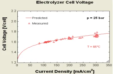
The model for the high pressure alkaline electrolyser shown in Fig. 3 is based on a combination of thermodynamics, heat transfer and empirical electrochemical equations. The electrochemical model is based on a temperature dependent I-U curve for a given pressure (Fig. 4) and a Faraday efficiency curve independent of temperature and pressure.
The electrode kinetics of an electrolyser cell is modelled using empirical I-U relationships. Overvoltages and ohmic resistance play an important role in the modelling of the I-U curve:
(
)
+
+
+
×
+
+
+
+
+
=
log
/
/
1
2 3 2 1 2 3 2 1 2 1
I
A
T
t
T
t
t
T
s
T
s
s
I
A
T
r
r
U
U
rev [image:2.595.315.513.607.737.2]being U the operation cell voltage (V), Urev the reversible cell voltage (V), ri the parameters for the ohmic resistance of electrolyte (Ω), siand ti the parameters for the overvoltage on the electrodes, A the electrode area (m2), T the temperature of the electrolyte (°C) and I the current through the cell (A).
Fig. 3. Scheme of a high pressure alkaline electrolyser
[image:2.595.87.303.611.699.2]Proton-Exchange Membrane Fuel Cell
The PEMFC model shown in Fig. 5 is largely mechanistic, with very theoretical basis.
The performance of a fuel cell is represented by its output voltage. The voltage of the single cell is calculated as:
ohmic act
cell E
U = +
η
+η
where E is the thermodynamic potential, ηact is the anode and cathode activation overvoltage (the voltage loss associated with the electrodes), and ηohmc is the ohmic overvoltage (the losses associated with the proton conductivity of the solid polymer electrolyte and electronic internal resistances).
E is defined through the Nernst equation:
(
)
(
0.5)
2 2 ln 0000431 . 0 298 00085 . 0 23 .
1 Tstack Tstack pH pO
E= − ⋅ − + ⋅ ⋅ ⋅
ηact is based on the theoretical equations from kinetic, thermodynamic and electrochemistry fundamentals:
(
)
0.000192 ln( )
0.000076 ln( )
2 ln 000192 . 0 00243 . 0 95 .0 stack stack PEM stack FC stack O
act =− + ⋅T + ⋅T ⋅ A − ⋅T ⋅ I + ⋅T ⋅ c
η
Finally, ηohmc is totally empirical, based on temperature and current experimental data:
⋅ + ⋅ + ⋅ − ⋅ ⋅ ⋅ − = 3 64 . 1 1 353 6 . 3 exp 8 PEM FC PEM FC stack stack PEM PEM FC ohmic A I A I T T A t I
γ
η
[image:3.595.152.454.620.706.2]Fig. 6 shows the cell voltage variation as a function of the current.
Fig. 5. Scheme of an PEM fuel cell
Fig. 6. Typical current-voltage curve for a PEMFC
Compressor
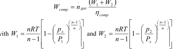
The compressor model is based on a two-stage polytropic compression process with intercooling. The total compression work for the process is given by:
(
)
comp gas comp W W n Wη
2 1 . + = with − − = − n n x P p n nRT W 1 1 1 11 and
− − = − n n x P p n nRT W 1 2 2 1 1
being ngas
.
the gas flow (mol.s-1), W1 and W2 the polytropic works (J.mol
-1
Gas storage
The compressed gas storage model calculates the pressure in the tank based on either the ideal gas law or van der Waals equation of state for real gases.
According to the ideal gas law, the pressure of a gas storage tank is given by:
V T R n
p= ⋅ ⋅ gas
For real gases, the Van der Waals equation of state indicates that the pressure of gas stored in a tank is:
2 2
V n a b n V
T R n
p gas − ⋅
⋅ −
⋅ ⋅ =
with
cr cr p
T R a
⋅ ⋅ ⋅ =
64
27 2 2
and
cr cr
p
T
R
b
⋅
⋅
=
8
where Tcr is the critical temperature (K) and pcr the critical pressure (Pa) of the gas. 3. Validation of the models
[image:4.595.211.382.205.287.2]The models described previously have been successfully validated using a combination of analytical tests and empirical comparisons. The analytic tests included the use of typical curves found in the literature and other energy systems modelling tools.
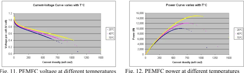
Fig. 7 and 8 show the current-voltage curve and the power curve obtained from the simulation of the Flagsol (KFA) 150 cell module at different temperatures. Fig. 9 presents the current-voltage curve of the same module at different solar radiation levels. At standard test conditions (25°C and 1000 W/m2 of solar radiation), the simulation indicates a 173.18 W maximum power point. Fig. 10 presents the effect of temperature on the simulated performance of the PHOEBUS alkaline electrolyser. Finally, the effect of temperature on the performance of a typical PEM fuel cell is simulated on Fig. 11 and 12.
Fig. 7. PV current at different temperatures Fig. 8. PV power at different temperatures
[image:4.595.85.505.477.723.2]Fig. 11. PEMFC voltage at different temperatures Fig. 12. PEMFC power at different temperatures
All these results are typical and verify the results available in the literature. They prove that the components models are accurate and that simulating hydrogen systems with TRNSYS provides reliable results.
4. Model Development and methodology
Models of four generic hydrogen systems based on the components models previously presented have been developed on the TRNSYS platform. The models cover the broad spectrum of prototype hydrogen demonstration systems emerging around the world. These are:
- a stand-alone power system - low power application - filling station
- energy buffering system for large scale renewables TRNSYS can be particularly tricky to
use. To make the models easier to use, TRNSED applications have also been designed. TRNSED is a customised interface that presents a simplified view of the TRNSYS file with only a few selected parameters available to users.
[image:5.595.265.518.382.564.2]A cost-benefit analysis model has been included to analyse the economic performance of the systems. The total net present cost of the system and the levelized cost of energy are calculated. The model also includes an optimisation method to optimise the technical and economic performance of the systems modelled.
Fig. 14. Flow chart of the optimisation process
5. Applications
The models have also been successfully applied to the analysis of two real systems: the HARI Project in Loughborough, UK and the Utsira Project in Norway.
Utsira is a small island community located approximately 18 kilometres off the west coast of Norway. The Utsira project is the world’s first full-scale stand-alone renewable energy system where the energy balance is provided by wind and stored hydrogen.
To be completed….
The application of the models improved confidence in their predictions and capabilities and also highlighted problems in the design and operation of the real and prospective systems including: poor control strategies, poor sizing of system components and mismatches of energy supply and demand.
6. References
TRNSYS 16, Volume 5, Mathematical Reference. University of Wisconsin-Madison, 2006
Rank the feasible solutions by total net present cost and select the cheapest one Create a parametric table with all the system configurations to be simulated
Run the simulation with the optimal sizes of components
Analyse the technical and economic performance of the optimal system Each feasible solution is saved Non-feasible ones are ignored
Repeat the optimisation process until a refined optimal system is found
The optimal configuration is found (Start)