Twisted Graph States for Ancilla-driven
Universal Quantum Computation
E. Kashefi
a, D. K. L. Oi
b, D. Browne,
cJ. Anders
cand E. Andersson
da School of Informatics, University of Edinburgh, Edinburgh EH8 9AB, UK bSUPA, Department of Physics, University of Strathclyde, Glasgow G4 0NG, UK cDepartment of Physics & Astronomy, University College London, London WC1E 6BT, UK
dSUPA, Department of Physics, Heriot-Watt University, Edinburgh EH14 4AS, UK
Abstract
We introduce a new paradigm for quantum computing called Ancilla-Driven Quantum Computation (ADQC) which combines aspects both of the quantum circuit [1] and the one-way model [2] to overcome challenging issues in building large-scale quantum computers. Instead of directly manipulating each qubit to perform universal quantum logic gates or measurements, ADQC uses a fixed two-qubit interaction to couple the memory register of a quantum computer to an ancilla qubit. By measuring the ancilla, the measurement-induced back-action on the system performs the desired logical operations.
The underlying mathematical model is based on a new entanglement resource calledtwisted graph states
generated from non-commuting operators, leading to a surprisingly powerful structure for parallel compu-tation compared to graph states obtained from commuting generators. [3]. The ADQC model is formalised in an algebraic framework similar to the Measurement Calculus [4]. Furthermore, we present the notion ofcausal flow for twisted graph states, based on the stabiliser formalism, to characterise the determinism. Finally we demonstrate compositional embedding between ADQC and both the one-way and circuit mod-els which will allow us to transfer recently developed theory and toolkits of measurement-based quantum computing and quantum circuit models directly into ADQC.
Keywords: Quantum computation, ancilla-driven, universal quantum computation, graph states
1
Introduction
There are two main paradigms which have driven both the theory and implemen-tation of quantum compuimplemen-tation; gate-based quantum computing (GBQC) [1], and measurement-based quantum computing (MBQC) [2]. Though these two models are computationally equivalent, in practice each has their own advantages and dis-advantages which have major implications for the choice of physical system, design, and operation. We introduce a new paradigm called ancilla-driven quantum com-puting which combines features of both mentioned models, in order to parallelise the architecture of quantum computers, to decrease decoherence effects, and simplify their physical implementation and operation.
1571-0661 © 2009 Elsevier B.V. Open access under CC BY-NC-ND license.
www.elsevier.com/locate/entcs
GBQC requires, in general, arbitrary dynamic global operations which in turn complicates the design and characterisation of the entire computer. Additionally it would be desirable to physically separate preparation, measurement, and co-herent interaction regions to reduce control complexity, circuitry congestion, and decoherence due to cross-talk. In contrast, MBQC performs computation purely through single-qubit measurement on a pre-existing static multi-partite entangled state, distilling and processing non-local correlation. However, the generation of the initial highly entangled state, incorporation of quantum error correction and fault-tolerance, and individual measurement of each qubit are issues in many candidate systems.
Our new model is partly inspired by the previous works of Andersson and Oi in [5], and also Perdrix and Jorrand in [6]. The first paper introduced an efficient method to implement any generalised quantum measurement by coupling the system with an ancilla qubit. However the method remains essentially similar to GBQC as it assumes arbitrary dynamic coupling operations between ancilla and system. On the other hand, the second paper describes a probabilistic version of MBQC in terms of a Turing machine where one can view the read-write head playing the role of an ancilla qubit, though this is not the way that the paper presents the model. Moreover this approach still directly manipulates the memory register and requires dynamic global measurement operators.
Ancilla-driven quantum computing (ADQC) attempts to overcome such issues by performing computation where the memory register (input data) can only be re-motely manipulated through interaction with a supply of prepared ancillas. In other words, instead of directly manipulating data qubits to perform universal quantum logic gates or measurements, ADQC uses a fixed two-qubit unitary interaction to couple the memory register of a quantum computer to an ancilla qubit. By mea-suring the ancilla, the measurement-induced back-action on the system performs the desired logical operation. Practically, a single fixed unitary interaction coupling the data and ancilla qubits greatly simplifies design, construction, and operation of the computer since only one particular discrete operation needs to be generated and characterised. Furthermore, separating interaction and measurement leads to a parallel structure with possibly reduced decoherence. A requisite interaction for universal ADQC already exists in a variety of physical systems ranging from ion micro-traps, neutral atoms, nuclear spin donors in semiconductors, SQUIDs and cavity QED which greatly increases the scope for implementation of the core ideas. ADQC also naturally benefits from optimisation of the qubit species employed for memory and ancilla. Memory qubits can be chosen for long coherence time at the expense of being static and difficult to manipulate directly, whilst ancilla qubits may be chosen for high mobility and rapid initialisation and measurement, e.g. donor nuclear spins in isotopically pure silicon as memory and electron spins conveyed via charge transport by adiabatic passage (CTAP) as ancilla in solid state quantum computing.
focus of the current paper, leads to the introduction of a new multi-partite entangle-ment resource. Only recently has it been demonstrated that a very restricted class of multi-partite entangled states are useful for universal deterministic MBQC [7,8]. However a full characterisation of such states [9] remains an open problem which this paper aims to make progress upon.
The entangled graph states [3] have emerged as an elegant and power-ful quantum resource, especially for measurement-based quantum computation (MBQC) [2]. Many important results on their entanglement properties [10], in-formation flow [11,12], implementation [13], and novel applications in cryptogra-phy [14,15], are due to their deceptively simple description. The generating operator for graph states, called controlled-phase, is a symmetric and commuting operator which leads to a simple graphical notation and hence the name for these states. Ad-ditionally, the elegant result by van de Nestet al. [16,10] shows that any stabiliser state is equivalent to a graph state up to local Clifford operators. This greatly expands the scope of these results and leads to a natural extension of the above constructions into stabiliser states, as well as allowing a convenient graphical no-tation for a very general class of states. If we consider open graph states, graph states where some nodes (called input nodes) are given in arbitrary states (rather than being prepared in a particular fixed state which is the case for graph states) much of the theory still follows. However open stabiliser states with arbitrary input nodes no longer fulfil the pre-requisites of the theorem by van de Nestet. al., and in general they do not admit a trivial graphical notation.
We address in this paper a particular class of open stabiliser states, calledtwisted graph stateswhich, despite having a non-commuting generator, still admits a simple graph representation. They form the key ingredient for ADQC. We then show how this new class of states can be viewed as open graph states up to some local swap operations. We also develop an algebraic framework similar to the measurement calculus, which is the mathematical framework underlying MBQC computation, to derive the standardisation theory for the ADQC patterns of computation. As we will see, any ADQC computation requires a classical control structure to compen-sate for the probabilistic nature of the measurement. We introduce the notion of
causal flow for twisted graph states based on the stabiliser formalism, to charac-terise the determinism. Compared to the open graph state, the stabiliser state has a more complicated and global structure. One can however sometimes construct computation within ADQC that is more parallel than other existing quantum mod-els. We will demonstrate this fact with a simple example. The full study of the parallel power of the model is, however, outside the scope of this paper. Finally we construct direct translations between ADQC and MBQC for a subclass of de-terministic patterns with flow. We also present the embedding between GBQC and ADQC and show how a separation in depth can be obtained.
2
Ancilla-Driven Model
As motivated in the introduction in ancilla-driven quantum computing we are in-terested in the following two essential properties:
• The only global operation is a fixed interaction between ancilla and system.
• Only ancilla qubits will be measured.
We introduce the ADQC model within an algebraic framework similar to that of the measurement calculus recalled in the appendix. We have a set of fixed basic commands described below where the indicesi,j,. . . represent the qubits on which each of these operations apply. A pattern is a sequence of commands defined over a set of qubits in the listV, called computation space, where the particular sub-list
S represents thesystem qubits (we may refer to them as data or memory register) and the restA=V \Sare theancilla qubits. In what follows we define an arbitrary pure single qubit state by
|+θ,φ= cos(θ2)|0+eiφsin(θ2)|1,
and denote its orthogonal state (the opposite point in the Bloch Sphere) with
|−θ,φ= sin(θ2)|0 −eiφcos(θ2)|1,
where 0≤θ≤π and 0≤φ≤2π.
• Preparation. Na|ψ (a∈A) prepares an ancilla qubit in the state|ψ.
• Interaction. Eas (s ∈ S, a ∈A) entangle a system qubit and an ancilla qubit with interaction operator controlled-Z followed by Hadamard on each qubit:
∧Z :=Hs⊗Ha∧Zas 1.
• Ancilla Measurement. Maλ,α (a ∈ A) measures qubit a on plane λ ∈
{(X, Y),(X, Z),(Y, Z)}, defined by orthogonal projections into:
· |±(X,Y),α:=|±π2,α ifλ= (X, Y)
· |±(X,Z),α:=|±α,0if λ= (X, Z)
· |±(Y,Z),α:=|±α,π2if λ= (Y, Z)
with the convention that|+θ,φ+θ,φ|acorresponds to the outcomema= 0, while
|−θ,φ−θ,φ|a corresponds to ma= 1. The propagation of dependent corrections (next command) defines dependent measurement:
n[Maλ,α]m:=Maλ,αXamZan
wherem, n, . . . are module 2 summation of several measurements outcomes, also called signals. Thedomain of a signal is the set of qubits on which it depends.2
1 We can also consider the interaction of the form controlled-Z + SWAP with the same initial ancilla and
measurements, similar results can be derived. The choice of interaction depends on the natural dynamics of the physical implementation
2 Depending on the context we sometimes use the notationmfor syntax, i.e., a set of qubits (representing
• Corrections. Xi andZi(i∈V), 1-qubit Pauli operators. As in MBQC, to con-trol the non-determinism of the measurement outcomes certain local corrections will depend upon previous measurement outcomes. These will be written as Cim, with Ci0=I, and Ci1=Ci.
We writeHV for the associated quantum state space ⊗i∈VC2. To run a pattern, one prepares the system qubits in some given input state Ψ∈HS, while the ancilla qubits are all prepared according to the N commands in fixed |ψ states. The commands are then executed in sequence, and finally the result of the pattern computation is read back from the system qubits3. Clearly, for this procedure to succeed, we had to impose the definiteness conditions as stated in the appendix.
The main differences between ADQC and MBQC are (1) The interaction op-erator being ∧Z instead of ∧Z, which still belongs to the normaliser of the Pauli group; (2) Only ancilla qubits can be measured, that is to say in the terminology of MBQC any ADQC pattern has the same number of inputs and outputs which are overlapping (system qubits). Apart from universality, which we will prove later, most of the theory of measurement calculus [4] which was developed for the one-way quantum computer can be easily adapted to ADQC. For completeness we briefly review this here.
The first way to combine patterns is by composing them. Two patternsP1 and P2 may be composed if S1 =S2. Provided that P1 has as many system qubits as P2 , by renaming these qubits, one can always make them composable. However it is important to emphasise that since theEij operators are non-commuting their order of appearance in each pattern must be preserved under the renaming and composition. The other way of combining patterns is to tensor them. Two patterns P1andP2may be tensored ifV1∩V2=∅. Again one can always meet this condition by renaming qubits in a way that these sets are made disjoint.
2.1 The semantics of patterns
We present a formal operational semantics for ADQC patterns as a probabilistic labelled transition system, similar to [4]. Besides quantum states, one needs a classical state recording the outcomes of the successive measurements one does in a pattern. If we letU stand for the finite set of qubits that are still active (i.e. not yet measured) and W stands for the set of qubits that have been measured (i.e. they are now just classical bits recording the measurement outcomes), it is natural to define the computation state space as:
C := ΣU,WHU ×ZW2 .
In other words the computation states form a U, W-indexed family of pairs q, Γ, whereqis a quantum state from HU and Γ is a map from some W to the outcome spaceZ2. We call this classical component Γ anoutcome map, and denote by∅the
3 Preparation and readout of the system qubits can be performed by using suitable ancilla states and
empty outcome map in Z∅2. We need further preliminary notation. For any signal
mand classical state Γ∈ZW2 , such that the domain ofmis included inW, we take
mΓto be the value ofmgiven by the outcome map Γ. That is to say, ifm=Imi, thenmΓ:=IΓ(i) where the sum is taken in Z2. Also if Γ∈ZW2 , andx∈Z2, we define
Γ[x/i](i) =x,Γ[x/i](j) = Γ(j) forj=i
which is a map in ZW2 ∪{i}.
We may now view each of our commands as acting on the state spaceC:
q,Γ N
|ψ i
−→ q⊗ |ψi,Γ
q,Γ −→Eeij ∧Zijq,Γ
q,Γ X
m i
−→ XmΓ
i q,Γ
q,Γ Z
m i
−→ ZmΓ
i q,Γ
U∪ {i}, W, q,Γ n[M
λ,α i ]m
−→ U, W ∪ {i},+λ,αΓ|iq,Γ[0/i]
U∪ {i}, W, q,Γ n[M
λ,α i ]m
−→ U, W ∪ {i},−λ,αΓ|iq,Γ[1/i]
where αΓ = (−1)mΓα+nΓπ. We introduce an additional command called signal
shifting:
q,Γ F
mΓ i
−→ q,Γ[Γ(i) +mΓ/i]
It consists in shifting the measurement outcome at i by the amount mΓ. Note that the Z-action leaves measurements globally invariant, in the sense that
|+α+π,|−α+π = |−α,|+α. Thus changing α to α +π amounts to replacing the outcomes of the measurements, and one has:
nΓ[M
α
i ]mΓ=FinΓ0[Miα]mΓ (1)
and signal shifting allows us to dispose of theZaction of a measurement, sometimes resulting in convenient optimisations of standard forms. In the rest of the paper, for simplicity, we omit the superscript Γ on the measurement outcomes.
The usual convention has it that when one does a measurement the resulting state is renormalised and the probabilities are associated with the transition. We do not adhere to this convention here, instead we leave the states unnormalized. The reason for this choice of convention is that this way, the probability of reaching a given state can be read off its norm, and the overall treatment is simpler.
2.2 Denotational Semantics
We now present the denotational semantics of ADQC patterns. If nis the number of measurements then the run may follow 2n different branches. Each branch is associated with a unique binary string n of length n, representing the classical outcomes of the measurements along that branch, and a unique branch map An
is obtained from the (un-normalised) operational semantics via the sequence (qi,Γi) with 1≤i≤m(wheremis the total number of commands), such that:
q1,Γ1 =q⊗ |+. . .+,∅
and for all i≤m:qi−1,Γi−1−→Ai qi,Γi.
and all measurement commands in the sequence{Ai}have been replaced by appro-priate projections corresponding to the outcome indexn.
Definition 2.1 A pattern P realizes a map on density matrices ρ given by ρ →
sAs(ρ)A†s. We write [[P]] for the map realised byP.
It is then easy to prove [4] that each pattern realizes a completely positive trace preserving (CPTP) map and if a pattern is strongly deterministic (see appendix), then it realizes a unitary embedding [4]. Hence the denotational semantics of a pattern is a CPTP-map. It is also compositional, as the following theorem shows.
Theorem 2.2 For two patternsP1andP2we have[[P1P2]] = [[P2]][[P1]]and[[P1⊗ P2]] = [[P2]]⊗[[P1]].
Proof. Recall that two patterns P1, P2 may be combined by composition
provided P1 has as many system qubits as P2. Suppose this is the case, and suppose further that P1 andP2 respectively realise some CPTP-mapsT1 and T2. We need to show that the composite pattern P2P1 realizes T2T1. Indeed, the two diagrams representing branches inP1 andP2:
HS1
/
/HS1 HS2
/
/HS2
HS1×Z∅2
p1//H
V1×Z∅2 //HS1×Z V1\S1
2
O
O
HS2×Z∅2
p2//H
V2×Z∅2 //HS2×Z V2\S2
2
O
O
can be pasted together, since S1 = S2, and HS1 = HS2. But then, it is enough
to notice 1) that preparation stepsp2 in P2 commute with all actions inP1 since they apply on disjoint sets of qubits, and 2) that no action taken in P2 depends on the measurements outcomes inP1. It follows that the pasted diagram describes the same branches as does the one associated to the composite P2P1. A similar argument applies to the case of a tensor combination, and one has that P2⊗P1 realizesT2⊗T1. 2
2.3 Generating patterns
The following one-parameter family J(α) generates all single-qubit unitary op-erators [17]:
J(α) := √1
2 ⎛ ⎝1 eiα
1 −eiα ⎞ ⎠
as any unitary operatorU onC2 can be written:
U =eiαJ(0)J(β)J(γ)J(δ)
for some α, β, γ and δ in R. Recall that the MBQC implementation of the J generator is:
J(−α) :=Xm1
a Ms(X,Y),αEsa (2)
where s is the system qubit input and a is the ancilla and Esa is controlled-Z operator [17]. On the other hand we can write the following pattern which also implements theJ gate but now the ancilla qubita will be measured
J(−α) :=HsZma
s Ma(Y,Z),αEsa (3)
whereHsrepresents the application of a Hadamard gate on the system qubit. We can now manipulate the new pattern to derive a generating pattern forJoperator in our model. Hence we have to get rid of theHsand replace the interaction command withEsa.
J(−α) :=HsZma
s Ma(Y,Z),αEsa =XsmaMa(Y,Z),αHsEsa
=XsmaMa(X,Y),αHaHsEsa
=Xma
s Ma(X,Y),αEsa (4)
Now we only need a generator for a two-qubit unitary such as controlled-Zto obtain the full universality but the MBQC pattern for controlled-Zij (Eij withi, j∈S) is not desirable as it is an operator between two qubits of the system rather than an interaction between system and ancilla qubits. Therefore the natural choice instead is to consider interaction of type EasEas and it is easy to check that the Pauli Z
measurement of the ancilla will give us a simple generating pattern for the two qubit operator∧Zss:
∧Z:=Xma
s MaZEasEas (5)
For simplicity, in the remainder of this paper we will restrict ourselves to a special class of patterns, namely, those using only ancillas of degree 1 with arbitrary (X, Y) plane measurement and of degree 2 with PauliZ measurement. However, the whole theory developed in this paper can be easily extended to the more general setting.
2.4 Standardisation
It is known that any MBQC model can admit a standardisation procedure if and only if the entangling command belongs to the normaliser group of the group gen-erated by the correction commands [12]. This is the case for our ADQC model and the following are the required rewrite rules:
EijXis=XjsZisEij (6)
EijZis=XisEij (7)
The rules for propagation of the correction through measurement are the same as for MBQC with additional rules for theMZ measurement:
n[Maα]mXap=n[Maα]m+p (8)
n[Maα]mZap=n+p[Maα]m (9)
MZ
aXam=FamMaZ (10)
MZ
aZam=MaZ (11)
We also have the same free commutation rewrite rules:
EijAk⇒AkEij whereAis not an entanglement (12)
AkXim⇒XimAk whereA is not a correction (13)
AkZim⇒ZimAk whereAis not a correction (14)
wherek represent the qubits acted upon by command A, and are distinct from i andj.
Recall that the effect of a Z correction on a qubit a simply flips the outcome of a measurement to be made on that qubit. Hence we can replace the dependen-cies induced by the Z correction by appropriate operations over the measurement outcomes as described below. In what follows m[n/mi] denotes the substitution ofmi with nin m wherem, nare modulo 2 summations of several measurement outcomes,
n[Maα]m=Fan[Maα]m (15)
XjmFin=FinXjm[n+mi/mi] (16)
ZjmFin=FinZjm[n+mi/mi] (17) n[Mjα]mFip=Fi np [p+mi/mi][Mjα]m[p+mi/mi] (18)
Fm
i Fjn=FjnFim[n+mj/mj]. (19)
It is important to emphasise the main difference between ancilla-driven and MBQC which is the interaction command Eij versus Eij. In order to achieve the desirable features of not directly measuring system qubits and having a fixed inter-action, we had to give up the simple operatorEij which is the generating operator of the open graph state.4 As we show in the appendix, for any standard pattern in MBQC we can write its underlying open graph state with qubits representing the nodes and Eij the edges of the graph. Then remarkably only from the geometry of this graph we can obtain the dependency structures to guarantee a determin-istic computation in MBQC. In other words the simple graph representation for the global operation defining pattern allows one to determine dynamic properties directly from the static structure. Can we still obtain similar properties for our new model? Despite the non-commutativity of Eij the answer is yes. In the next section we define the twisted graph state which is the underlying geometry of a given ancilla-driven pattern obtained from standardisation and we present how one can directly construct the dependency structure from their geometry.
3
Twisted Graph States
The main issue with the Eij operators is the fact that they are non-commuting, therefore after standardisation their order will be important. Another important property of an ancilla-driven pattern is that system qubits interact only with an-cilla qubits. Therefore we introduce a multipartite entangled state as a graph over ancilla and system qubits and Eij edges with extra condition to address the above mentioned requirements. In Section 4.2 we show how this new class of states can be viewed as open graph states up to some local swap operators. This is the reason behind the chosen name.
Definition 3.1 An open twisted graph state (G, S, A,C) consists of a bipartite graph G over disjoint sets of qubits S and A, called systems and ancillas, such that the maximum degree of any ancilla node is 2, together with an edge labelling
C. The labels define a partial ordering over edges where the order is total and strict on any edges that share a common vertex,i.e.it defines an edge colouring.
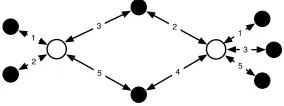
The corresponding quantum state, denoted as |EG, is obtained by preparing qubits in S in given arbitrary states and all the qubits in A in the |+ state, and then applyingEij over corresponding qubits according to the partial order ofC (see Figure1).
One may think of an open twisted graph state as the beginning of the definition of an ancilla-driven pattern, where one has already decided how many qubits will be used (V =S∪A) and how they will be entangled:
EG:= {i,j}∈E˜Eij.
4 Informally speaking this is due to the fact that usingEijand ancilla measurement one cannot implement
1
5 2
3
5 3 1
2
[image:11.468.166.308.65.118.2]4
Fig. 1. An open twisted graph state where the system qubits are the white circles that will not be measured and the rest are ancilla qubits. The edges areEeinteractions and edge labels denote the partial order.
To complete the definition of the pattern it remains to decide which angles will be used to measure ancilla qubits and, most importantly if one is interested in deter-minism, which dependent corrections will be applied. Conversely, any ancilla-driven pattern has a unique underlying open twisted graph state obtained by forgetting measurements and corrections where the colour of the edges is given by the most partial order of theEij commands which respects the non-commuting order. Recall that twoEij commands commute if and only if they act on disjoint set of qubits. Note that the depth of this partial order is the true depth of the preparation of the state.
Different ordered colourings over the same graph structure might lead to different twisted graph states and consequently different patterns of computation. We leave as an open question whether one can find a more relaxed definition that can still uniquely define the entangled state corresponding to an ancilla-driven pattern. On the other hand our restrained definition will allow us to derive the dependency structure of the measurements directly from the order of the colouring, this is the topic of the next subsection.
3.1 Dependency structure
We will use the graph stabiliser formalism [18,3] to construct a deterministic pattern. Recall that for any open graph state |EG defined over a graphG with vertices V, we have the following set of equations for all the non-input qubits:
Xi j∈G(i)Zj(|EG) =|EG
whereG(i) is the set of neighbour vertices ofi inG. The above Pauli operators are called the stabiliser operators of|ψ.
Similarly we define the stabiliser operators of a given twisted graph state |EG defined over a graphGwith verticesV =S∪A. We will use the following notation as well. Define S(a) for a ∈ A to be the attached system qubit s ∈ S with the smallest edge label and S(a) to be the other one if it exists;N(s) fors∈S to be the set of ancilla qubits connected to the system qubit s; and finally GS(a) to be the sub-graph with edges betweenS(a) andNS(a).
Consider first a simple case whereEG=EaS(a)Na|+. Then the stabiliser has the form
The above equation is due to
ZaXS(a)(EaS(a)Na|+) = EaS(a)XaZS(a)ZS(a)Na|+ = EaS(a)Na|+
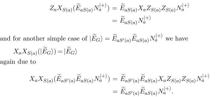
and for another simple case of|EG=EaS(a)EaS(a)Na|+ we have
XaXS(a)(|EG) =|EG (21) again due to
XaXS(a)(EaS(a)EaS(a)N| +
a ) = EaS(a)EaS(a)XaZS(a)ZS(a)Na|+
= EaS(a)EaS(a)Na|+.
In order to generalise the above cases the following rewrite rules for Pauli com-mutations will be used:
• Equation 6,EijXis=XjsZisEij, transforms theX operation on the system qubit to the next immediate ancilla qubit, introducing a Z operation at the system qubit.
• Equation 7, EijZis= XisEij, replaces the Z operation on the system qubit with anX operation.
Unlike the stabiliser of the graph state which has a local structure, in the case of a twisted graph state the stabiliser ofaaffects the whole of the graph. This action is, however, recursive and can be defined using the collection of several local actions. Define the label of an ancilla node to be the same as the label of the edge EaS(a). Consider an ancilla qubit a and those qubits in N(S(a)) with label greater than label of a (see Figure2). We can assume, without loss of generality, that all edges connected to S(a) have labels 1 to n with 1 being the label of a. This is due to the fact that the stabiliser ofahas an effect only on those qubits inN(S(a)) where their edge interaction are after the edge interaction of a and S(a) hence having a greater edge label.
2
n 1
3 a
[image:12.468.40.386.82.237.2]S(a)
Fig. 2. The generic case for the local study of stabiliser at ancillaa.
Definition 3.2 Given a twisted graph state (G, S, A,C), a local stabiliser on the ancilla qubita is defined as following:
• AddX on vertices inN(S(a)) with even label and degree 1.
• AddZ on vertices inN(S(a)) with even label and degree 2.
• AddX on the system qubit if nis odd otherwise addZ.
We denote the above set of Pauli operators withPl(S(a)) which acts on a subset of qubits inN(S(a)).
DefineI(a) to be the set of degree-two ancilla qubits inN(S(a)) with even label that get aZPauli operator in the definition of the local stabiliser ofa. The stabiliser ofa will have the same local effect as defined above over S(a) for all thea∈I(a) and the same structure repeats for vertices inI(a). Therefore we define recursively such qubits
I∗(a) ={a|∃n:a∈In(a)} whereI1(a) =I(a) andIn+1(a) =
a∈In(a)I(a). We can now present a recursive
definition for the stabiliser of a twisted graph state as the product of a collection of local stabilisers.
Definition 3.3 Given a twisted graph state (G, S, A,C), the stabiliser on the an-cilla qubita is defined as follows:
P(a) = Za a∈I∗(a)Pl(S(a)) if ahas degree one
P(a) = Xa a∈I∗(a)Pl(S(a)) otherwise
It is a straightforward but cumbersome computation to show the correctness of the above definition and we omit the details of the proof.
We can now adapt the notion of flow and generalised flow of graph states [11,12] for twisted graph states to derive a sufficient condition for determinism. The key idea is exactly the same as in the MBQC case based on the following simple obser-vation. We could make a measurement Mi(X,Y),α “deterministic” (corrected) if it could be pre-composed by an anachronical Zsi
i correction (i.e. conditioned on the outcome of a measurement which hasn’t happened yet). This unphysical scenario is a useful starting point for our proof.
+(X,Y),α|a = Ma(X,Y),αZma
a
The flow construction guarantees that a deterministic pattern with anachronical corrections
P = Ca∈A +(X,Y),α|a EG
= Ca∈A Ma(X,Y),αZma
a EG
composed with the anachronical correction, forms an operator which commutes with the measurement, and thus the pattern can be brought into runnable order.
For simplicity in the rest of the paper we consider only patterns where degree-two vertices are measured with Pauli Z and degree-one vertices are measured in the (X, Y) plane, we use the generic term Maλa,αa for both cases. This class of patterns are large enough to introduce a universal ADQC model as they include the generating pattern introduced in Section 2.3. However the definition of flow and determinism can be extended to the more general case as well.
Definition 3.4 An open twisted graph state (G, S, A,C) has causal flow if there exists a partial order > over V consistent with the ordering ofC such that for all
a ∈ A and all vertices a ∈ P(a) we have a < a except for those a that will be measured with PauliZ.
Theorem 3.5 Suppose the open twisted graph state (G, S, A,C) has a causal flow with the partial order >. Define:
C(a) = P(a)Za for all degree-one ancilla a
C(a) = P(a)Xa for all degree-two ancilla a
then the pattern:
PG,α := >a∈A C(a)ma Maλa,αa EG
where the product follows the dependency order >, is runnable, uniformly and strongly deterministic.
Proof. The proof is based on the following equations first consider the (X, Y) measurement case for degree-one ancillas:
+α|a(EG) = MaαZma
a (EG)
= MaαZma
a P(a)ma(EG)
= C(a)maMα
a(EG)
Similarly for theZ measurement over degree-two ancillas we have:
0|a(EG) = MaZXma
a (EG)
= MaZXma
a P(a)ma(EG)
= C(a)maMZ
a(EG)
Hence we can write:
>
a∈Aλa, αa|aEG= >a∈A C(a)ma Maλa,αa EG.
order > except for the Z correction introduced over degree-two ancillas. However one can ignore them since these qubits will be measured with PauliZ and we have
MZ
a Zam=MaZ. This finishes the proof. 2
It is interesting to note that the flow definition for a graph state was based on the geometry of the underlying graph, whereas in a twisted graph state it is based on the edge colouring order. Indeed, as mentioned before, different edge colourings lead to different twisted graph states and hence different flow constructions. Roughly speaking, the edge colouring plays the role of geometry for the twisted graph states.
4
Compositional Embedding
One of the main foci in constructing direct translations between models is to study parallelism as the more parallel the computation, the more robust it is against decoherence. Recently the advantage of MBQC over GBQC in terms of depth complexity has been demonstrated where a logarithmic separation was shown [19]. Furthermore it is also known that the parallel power of MBQC is equivalent to GBQC equipped with quantum fan-out gates [20]. Such a full analysis for ADQC is outside the scope of this paper. We will only present the transformations between ADQC and other models which could be used for pattern synthesis and present only an example on how ADQC could be more parallel.
4.1 GBQC and ADQC
The question of translating GBQC circuits into MBQC patterns and vice versa has been addressed before in [19] and it can be directly adapted for ADQC as well. In fact the universality proof of ADQC already presents a method of translation of a circuit into ADQC: (I) Rewrite the given circuit in terms of the universal gates set ofJ(α) and ∧Z; (II) Replace each gate with its corresponding ADQC pattern (equations4and5); (III) Perform the standardisation procedure.
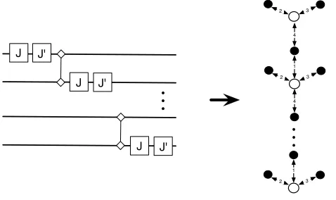
The above construction cannot be used in reverse as the edge colouring order might lead to a circuit with an acausal loop. However it is possible to keep all the auxiliary qubits to avoid creating loops in the resulting circuit. The scheme is simply based on the well-known method of coherently implementing a measurement [19]. It is also easy to prove, in a similar way as in [19], that the translation from a GBQC circuit into an ADQC pattern will never increase the depth as the number of the edge colouring number of the obtained twisted graph state will be upper-bounded by the depth of the original circuit. More importantly, we present an example where the depth decreases exponentially. Consider the ladder structure of the circuit in Figure3which has depthn. This circuit, through the introduced construction, will be translated into a pattern with the twisted graph state shown in Figure3which has constant depth 4. This is due to the simple fact that both the computation and preparation depths for any ADQC pattern are upper bounded by the edge colouring of the graph, which in this case is equal to 4.
How-1 4
3 2
3 2
4
1 3 2
J' J
J' J
[image:16.468.115.354.64.206.2]J J'
Fig. 3. A ladder structure circuit with the binary∧fZ gates and the unitaryJ(α) gates, together with the corresponding open twisted graph state obtained via gate by gate translation.
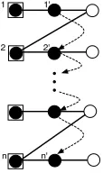
ever the nature of the above example differs from the class of circuits that can be parallelised via a translation into MBQC. In fact a direct translation of the above example will lead to a pattern of depthn (see Figure 4). Hence the example sug-gests that we might achieve more parallelism in the ADQC model in comparison to GBQC and MBQC and a detailed study of depth complexity in ADQC might reveal further new techniques in parallelising GBQC as it was done for MBQC [19].
4.2 MBQC and ADQC
As mentioned before there exists a compositional embedding from MBQC patterns with flow into GBQC and vice versa, and together with the construction of the last subsection one can obtain an embedding between ADQC and MBQC for patterns with flow. However in view of parallelism, it is interesting to find such an embedding directly by presenting the correspondence between twisted open graph states and open graph states.
The following equation relates the two resources but it is only valid for degree-one ancilla qubits
EasNa|+= SWAPa,sEasNa|+ (22)
where SWAPa,sis the unitary operator swapping qubitsaands. This equation and the next one are in fact the reason behind the chosen name for this class of states as one can recover a graph state from them by applying the appropriate sequence of twist operators. In order to handle the degree-two ancilla qubits we will use the following pattern equations
∧Z:=Xma
s MaZEasEas
= Xma
s MaZHaHsEasEas
= Xma
s MaXHsEasEas
= Xmb
s XsmaMaXMbXEbsEasEas (23)
In the new pattern for ∧Z both instances of Eas can be replaced using Equation
degree-two vertices are measured with Pauli Z, into a pattern over a graph state obtained through the above manipulations of theEas edges.
1
2
n n' 1'
[image:17.468.210.267.99.195.2]2'
Fig. 4. The MBQC pattern obtained from the direct translation of the circuit in Figure3. The pattern has depthndue to the sequence of dependent measurements (the doted lines).
The other direction of translation between patterns, from MBQC into ADQC, is an open problem. One can of course translate any MBQC pattern with flow first into a GBQC circuit and then to a corresponding ADQC but we believe a direct embedding, if it can be found, can reveal more insights on parallelism and also the relationship between commuting graph states and non-commuting twisted graph states as resources. We finish this section by pointing out again that an ADQC pattern might be indeed more parallel than the corresponding MBQC one. Recall the ladder circuit in Figure3, where the corresponding ADQC pattern had constant depth 4. Now as shown in Figure4the depth of the MBQC pattern obtained from a direct translation will ben due to the sequence of the X dependencies between measurements on qubits 1,2,· · ·, n. This begs the question of direct translation between MBQC and ADQC and a careful analysis of depth trade off. We leave as a conjecture that one might find a logarithmic depth separation between these two models.
5
Discussion
5.1 Physical Implementations
qubits or a “read/write” head. For example, an optical lattice of neutral atoms can be addressed by a separately controlled atom [21,22]. Since it is difficult to individ-ually address with lasers a single site of a fully filled optical lattice, the read-write head would interact with selected sites and can be used as the ancilla. A similar idea can be applied to neutral atoms trapped in dipole trap arrays [23] controlled by an atom in an optical tweezer [24]. Similarly in [25], ions in an array of micro traps would be manipulated by a single ion read-write head. Alternatively in [26], the role of the memory is played by the quantised electromagnetic field in an array of cavities whilst Rydberg atoms traversing the cavities act as ancillas (similar ideas are contained in [27]). All of the above schemes possess a natural control-Z (dis-persive) interaction between the ancilla and system qubits. For universality, either an additional Hadamard operation on the system should be incorporated into this interaction (e.g. through the pushing laser in [25]), or an effective SWAP operation be found in conjunction with the Controlled-Z. The latter could be achieved through cold collisions between ancilla and system [28,29].
A system which may prove particularly amenable to our model is one based on [30]. Here, the nuclear spin of a single dopant atom in isotopically pure silicon plays the role of a memory qubit which can be controllably coupled via the hyper-fine interaction to an electron spin which acts as an ancilla qubit. Nuclear spins can be very well isolated from the environment, as well as the state preparation and measurement areas. Electrons can be rapidly transported around the computer using charge transport via adiabatic passage (CTAP), this avoids the issue of swap-ping nuclear spin states, as in the original Kane proposal [31], which can lead to a reduction in fault tolerance. An issue here is making sure that the interaction between electron and nuclear spins is of the correct form as to allow conditional unitary dynamics5. A controlled-Z + SWAP gate can be achieved by using the method presented in [32] with only the Heisenberg interaction between ancilla and system and local operations on the ancilla itself.
A natural interaction which is also suitable for ADQC is the XY-Hamiltonian which be easily turned into the controlled-Z + SWAP gate [33] (equivalent to the ISWAP in the aforementioned reference). In [34], a natural XY-interaction between nuclear spins, as in the Kane proposal, is mediated by a 2D electron gas in the Quantum Hall regime. The XY-interaction also naturally occurs between quantum dots coupled by a cavity [35] or superconducting qubits [36,37]. Here, the memory and ancilla qubits are of the same species.
5.2 Open Problems
The model for ADQC presented here has been based upon either ∧Z := Hs⊗
Ha∧Zas or control-Z + SWAP. These interactions have the useful property of per-mitting unitary conditional measurement-induced back-action. However, this prop-erty is shared by a more general class of interactions. It is an open problem as to
5 In order for the conditional measurement-induced back-action on the system to be unitary, the non-local
which interactions lead to universal ADQC. We may even look at generalising our computational models to dispense with determinism (whether different branches of the computation can be corrected by simple Pauli operators) or even unitarity at each stage.
More generally, it is interesting to expand the set of resource states universal for quantum computation [7,8]. Different interactions may lead to different classes of states, together with their own measurement calculus. We can envisage connecting the resource states for universal MBQC with physical interactions which generate them, and hence the type of correlations which are induced. From the ADQC embedding, we can trace the roles of measurement-induced back-action and the non-local character of the generating interaction.
6
Conclusion
Ancilla-Driven Quantum Computation presents a new way of performing universal quantum computing. Aside from potential advantages for quantum computer con-struction and operation, it leads to a new set of universal quantum computational resources, the twisted graph state, based upon a non-commuting generating interac-tion. The measurement calculus has been developed to encompass this new model and even greater parallelism compared to conventional MBQC may be possible. Despite the non-commuting nature of the generating interaction for twisted-graph states, the graphical structure still encodes the dynamics (dependancy structure) of the computation. A strong possibility is that ADQC could further improve the parallelism of MBQC. By further studying ADQC and its generalisations, further insight into this question could be achieved.
References
[1] D. Deutsch. Quantum computational networks. Proc. Roy. Soc. Lond A, 425, 1989.
[2] R. Raussendorf and H. J. Briegel. A one-way quantum computer.Physical Review Letters, 86, 2001. [3] M. Hein, J. Eisert, and H. J. Briegel. Multi-party entanglement in graph states. Physical Review A,
69, 2004. quant-ph/0307130.
[4] V. Danos, E. Kashefi, and P. Panangaden. The measurement calculus. Journal of ACM, 2007. [5] E. Andersson and D. K. L. Oi. Binary search trees for generalized measurements. Physical Review A,
77(5, Part A), 2008.
[6] S. Perdrix and P. Jorrand. Measurement-based quantum Turing machines and their universality. quant-ph/0404146, 2004.
[7] D. Gross, S. Flammia, and J. Eisert. Most quantum states are too entangled to be useful as computational resources. arXiv:0810.4331v2, 2008.
[8] M. J. Bremner, C. Mora, and A. Winter. Are random pure states useful for quantum computation? arXiv:0812.3001v1, 2008.
[9] D. Gross, J. Eisert, N. Schuch, and D. Perez-Garcia. Measurement-based quantum computation beyond the one-way model. Physical Review A, 76, 2007.
[11] V. Danos and E. Kashefi. Determinism in the one-way model. Physical Review A, 2006.
[12] D. Browne, E. Kashefi, M. Mhalla, and S. Perdrix. Generalized flow and determinism in measurement-based quantum computation. New Journal of Physics, 9, 2007.
[13] S. D. Barrett and P. Kok. Efficient high-fidelity quantum computation using matter qubits and linear optics.Physical Review A, 71, 2005.
[14] D. Markham and B. C. Sanders. Graph states for quantum secret sharing. Physical Review A, 78(4), 2008.
[15] A. Broadbent, J. Fitzsimons, and E. Kashefi. Universal blind quantum computation. arXiv:0807.4154v1, 2008.
[16] M. Van den Nest, J. Dehaene, and B. De Moor. An efficient algorithm to recognize local clifford equivalence of graph states. Physical Review A, 70, 2004. quant-ph/0405023.
[17] V. Danos, E. Kashefi, and P. Panangaden. Parsimonious and robust realizations of unitary maps in the one-way model.Physical Review A, 72, 2005.
[18] M. A. Nielsen and I. L. Chuang. Quantum Computation and Quantum Information. Cambridge University Press, 2000.
[19] A. Broadbent and E. Kashefi. On parallelizing quantum circuits. quant-ph/0704.1736, 2007.
[20] D. Browne and S. Perdrix. On the computational power the measurement-based quantum computing. Private communication, 2009.
[21] L You and MS Chapman. Quantum entanglement using trapped atomic spins. Physical Review A, 62(5):art. no.–052302, 2000.
[22] T Calarco, U Dorner, PS Julienne, CJ Williams, and P Zoller. Quantum computations with atoms in optical lattices: Marker qubits and molecular interactions.Physical Review A, 70(1), 2004.
[23] R Dumke, M Volk, T Muther, F.B.J. Buchkremer, G Birkl, and W Ertmer. Micro-optical realization of arrays of selectively addressable dipole traps: A scalable configuration for quantum computation with atomic qubits.Physical Review Letters, 89(9), 2002.
[24] J. Beugnon, C. Tuchendler, H. Marion, A. Gaetan, Y. Miroshnychenko, Y. R. P. Sortais, A. M. Lance, M. P. A. Jones, G. Messin, A. Browaeys, and P. Grangier. Two-dimensional transport and transfer of a single atomic qubit in optical tweezers. Nature Physics, 3(10):696–699, 2007.
[25] J.L. Cirac and P. Zoller. A scalable quantum computer with ions in an array of microtraps. Nature, 404(6778):579–581, 2000.
[26] V Giovannetti, D Vitali, P Tombesi, and A Ekert. Scalable quantum computation with cavity QED systems.Physical Review A, 62(3), 2000.
[27] P. J. Blythe and B. T. H. Varcoe. A cavity-QED scheme for cluster-state quantum computing using crossed atomic beams. New Journal of Physics, 8, 2006.
[28] E Charron, E Tiesinga, F Mies, and C Williams. Optimizing a phase gate using quantum interference.
Physical Review Letters, 88(7), 2002.
[29] K Eckert, J Mompart, XX Yi, J Schliemann, D Bruss, G Birkl, and M Lewenstein. Quantum computing in optical microtraps based on the motional states of neutral atoms.Physical Review A, 66(4), 2002. [30] AD Greentree, JH Cole, AR Hamilton, and LCL Hollenberg. Coherent electronic transfer in quantum
dot systems using adiabatic passage. Physical Review B, 70(23), 2004.
[31] BE Kane. A silicon-based nuclear spin quantum computer. Nature, 393(6681):133–137, 1998. [32] D Loss and DP DiVincenzo. Quantum computation with quantum dots.Physical Review A, 57(1):120–
126, 1998.
[33] N Schuch and J Siewert. Natural two-qubit gate for quantum computation using the XY interaction.
Physical Review A, 67(3), 2003.
[34] D Mozyrsky, V Privman, and ML Glasser. Indirect interaction of solid-state qubits via two-dimensional electron gas.Physical Review Letters, 86(22):5112–5115, 2001.
[36] J Siewert, R Fazio, GM Palma, and E Sciacca. Aspects of qubit dynamics in the presence of leakage.
J. Low Temperature Physics, 118(5-6):795–804, 2000. International Conference on Electron Transport in Mesoscopic Systems (ETSM ‘99), GOTHENBURG, SWEDEN, AUG 12-15, 1999.
[37] L.S. Levitov, T.P. Orlando, J.B. Majer, and J.E. Mooij. Quantum spin chains and majorana states in arrays of coupled qubits. arXiv:cond-mat/0108266v2, 2001.
[38] R.P. Feynman. Simulating physics with computers. International Journal of Theoretical Physics, 21, 1982.
[39] D. Deutsch. Quantum theory, the Church-Turing principle and the universal quantum computer. In
Proceedings of the Royal Society of London, volume A400, 1985.
[40] R. Raussendorf and H. J. Briegel. Computational model underlying the one-way quantum computer.
Quantum Information & Computation, 2, 2002. quant-ph/0108067.
[41] R. Raussendorf, D. E. Browne, and H. J. Briegel. Measurement-based quantum computation on cluster states. Physical Review A, 68, 2003.
[42] Richard Jozsa. An introduction to measurement based quantum computation. quant-ph/0508124, 2005.
[43] M. A. Nielsen. Cluster-state quantum computation. Reviews in Mathematical Physics, 2005. quant-ph/0504097.
[44] D. E. Browne and H. J. Briegel. One-way quantum computation - a tutorial introduction. quant-ph/0603226, 2006.
A
Preliminaries
We briefly review the required concepts from quantum computing, a more detailed introduction can be found in [18]. Let H denote a 2-dimensional complex vector space, equipped with the standard inner product. We pick an orthonormal basis for this space, label the two basis vectors|0 and|1, and for simplicity identify them
with the vectors ⎛
⎝1
0 ⎞
⎠ and
⎛
⎝0
1 ⎞
⎠, respectively. Aqubit is a unit length vector in
this space, and so can be expressed as a linear combination of the basis states:
α0|0+α1|1= ⎛ ⎝α0
α1 ⎞ ⎠.
Hereα0, α1 are complexamplitudes, and|α0|2+|α1|2= 1.
Anm-qubit state is a unit vector in the m-fold tensor space H ⊗ · · · ⊗ H. The 2m basis states of this space are the m-fold tensor products of the states |0 and
|1. We abbreviate |1 ⊗ |0 to |1|0 or |10. With these basis states, anm-qubit state |φ is a 2m-dimensional complex unit vector
|φ=
i∈{0,1}m
αi|i.
We use φ| = |φ∗ to denote the conjugate transpose of the vector |φ, and
φ | ψ = φ| · |ψ for the inner product between states |φ and |ψ. These two states are orthogonal ifφ|ψ= 0. Thenorm of|φis||φ||=φ|φ.
A quantum state can evolve by a unitary operation or by a measurement. A
unitary transformation is a linear mapping that preserves the norm of the states. If we apply a unitaryU to a state |φ, it evolves to U|φ. ThePauli operators are a well-known set of unitary transformations for quantum computing:
X = ⎛ ⎝0 1
1 0 ⎞
⎠, Y =
⎛ ⎝0 −i
i 0 ⎞
⎠, Z=
⎛
⎝1 0
0 −1 ⎞ ⎠,
and the Pauli group on n qubits is generated by Pauli operators. Several other unitary transformations that we will use in this paper are: the identityI, thephase
gate P(α), of which P(π/4) and P(π/2) are a special cases, the HadamardH and the controlled-Z (∧Z):
I := ⎛ ⎝1 0
0 1 ⎞
⎠ P(α) :=
⎛
⎝1 0
0 eiα ⎞
⎠ H := √1
2 ⎛
⎝1 1
1 −1 ⎞ ⎠
∧Z:= ⎛ ⎜ ⎜ ⎜ ⎜ ⎜ ⎜ ⎝
1 0 0 0
0 1 0 0
0 0 1 0
0 0 0−1 ⎞ ⎟ ⎟ ⎟ ⎟ ⎟ ⎟ ⎠
SW AP := ⎛ ⎜ ⎜ ⎜ ⎜ ⎜ ⎜ ⎝
1 0 0 0
0 0 1 0
0 1 0 0
0 0 0 1 ⎞ ⎟ ⎟ ⎟ ⎟ ⎟ ⎟ ⎠
The Clifford group on n qubits is generated by the matrices Z, H, P(π/2) and
∧Z, and is the normaliser of the Pauli group. This set of matrices is not universal for quantum computation, but by adding any single-qubit gate not in the Clifford group (such asP(π/4)), we do get a set that is approximately universal for quantum computing.
The most general measurement allowed by quantum mechanics is specified by a family of positive semi-definite operators Ei = Mi∗Mi, 1 ≤ i ≤ k, subject to the condition that iEi = I. A projective measurement is defined in the spe-cial case where the operators Ei are projections. Let|φ be an m-qubit state and
B = {|b1, . . . ,|b2m} an orthonormal basis of the m-qubit space. A projective measurement of the state |φ in the B basis means that we apply the projection operators Pi = |bibi| to |φ. The resulting quantum state is|bi with probability
pi =|φ |bi|2. An important class of projective measurements are Pauli measure-ments, i.e.projections to eigenstates of Pauli operators.
So far we have dealt with pure quantum states. A more general representation with density matrices also allows us to describe open physical systems, where one can prepare a classical stochastic mixture of pure quantum states, called mixed
projection operator |ψψ|. Suppose that we only know that a system is one of several possible states |ψ1, . . . ,|ψk with probabilities p1, . . . , pk respectively. We define the density matrix for such a state to be
ρ= k
i=1
pi|ψiψi|.
The most general physical operator that acts over density matrices is a completely positive trace preserving map (CPTP)E :B(H1)→ B(H2) with Kraus decomposi-tion
E(ρ) = m
AmρA†m
where the Am : H1 → H2, B(H) is the Banach space of bounded linear operators
and we require that
m
A†mAm=I
A.1 Quantum circuit model
Richard Feynman was one of the first to suggest that a computer based on the prin-ciples of quantum mechanics could efficientlysimulate other quantum systems [38]. David Deutsch then developed the idea that the quantum computer could offer a computational advantage compared to a classical computer; he also defined the
quantum Turing machine [39], before defining the quantum circuit model [1] to represent quantum computations.
Any unitary operation U can be approximated with a circuit C, using gates from a fixed universal set of gates. Thesize of a circuit is the number of gates and its depth is the largest number of gates on any input-output path. Equivalently, the depth is the number of layers that are required for the parallel execution of the circuit, where a qubit can be involved in at most one interaction per layer. In this paper, we adopt the model according to which at any given time-step, a single qubit can be involved in at most one interaction. This differs from theconcurrency
viewpoint, according to which all interactions for commuting operations can be done simultaneously.
A.2 Measurement-based model
We give a brief introduction to measurement-based quantum computing
(MBQC) [2,40,41], a more detailed description is available in [42,43,44,4] and our notation follows that of [4]. In MBQC, computations are represented as patterns, which are sequences ofcommands acting on the qubits in the pattern. These com-mands are of four types:
(i) Ni is a one-qubit preparation command which prepares the auxiliary qubit i in state |+= √1
(ii) Eij is a two-qubit entanglement command which applies the controlled-Z op-eration, ∧Z, to qubits i and j. Note that the ∧Z operation is symmetric and so Eij = Eji. Also, Eij commutes with Ejk and so the ordering of the entanglement commands in not important.
(iii) Miα is a one-qubit measurement on qubit i which depends on parameter α∈ [0,2π) called theangle of measurement. Miα is the orthogonal projection onto states
|+α= √1
2(|0+e iα|1)
|−α= √1
2(|0 −e iα|1),
followed by a trace-out operator, since measurements are destructive. We denote the classical outcome of a measurement performed at qubitibymi∈Z2. We take the specific convention that mi = 0 if the measurement outcome is|+α, and thatmi = 1 if the measurement outcome is|−α. Outcomes can be summed together resulting in expressions of the form
m= i∈I
mi
which are calledsignals, and where the summation is understood as being done modulo 2. Thedomain of a signal is the set of qubits on which it depends (in this example, the domain ofm isI).
(iv) Xi andZi are one-qubit Pauli corrections which correspond to the application of the PauliX andZ matrices, respectively, on qubiti.
In order to obtain universality, we have to add a classical control mechanism called feed-forward, which allows measurement angles and corrections to be de-pendent on the results of previous measurements [2,4]. Let m and n be signals. Dependent corrections are written asXim andZin and dependent measurements are written asn[Miα]m. The meaning of dependencies for corrections is straightforward:
X0
i =Zi0=I (no correction is applied), whileXi1=XiandZi1=Zi. In the case of dependent measurements, the measurement angle depends onm,nandαas follows:
n[Miα]m=M(−1)
mα+nπ
i (A.1)
so that, depending on the parity of mandn, one may have to modify the angle of measurement α to one of −α, α+π and−α+π. These modifications correspond to conjugations of measurements underX andZ:
XimMiαXim =M(−1)
mα
i (A.2)
Zn
iMiαZin =Miα+nπ (A.3)
and so we will refer to them as theX- andZ-actions or alternatively as theX- and
to:
MiαXim=M(−1)
mα
i (A.4)
MiαZin=Miα+nπ. (A.5)
Note that these two actions are commuting, since−α+π=−α−π up to 2π, and hence the order in which one applies them does not matter.
Apattern is defined by the choice of a finite set V of qubits, two not necessarily disjoint sets I ⊆V andO⊆V determining the pattern inputs and outputs, and a finite sequence of commands acting onV. We require that no command depend on an outcome not yet measured, that no command act on a qubit already measured, that a qubit be measured if and only if it is not an output qubit and that a qubit be prepared if and only if it is not an input qubit. This set of rules is known as the
definiteness condition.
A pattern is said to be in standard form if all the preparation commands Ni and entanglement operatorsEij appear first in its command sequence, followed by measurements and finally corrections. A pattern that is not in standard form is called awild pattern. Any wild pattern can be put in its unique standard form [4]; this form can reveal implicit parallelism in the computation. The procedure of rewriting a pattern in its standard form is calledstandardisation. This can be done by applying the following rewrite rules:
EijXim⇒XimZjmEij (A.6)
EijZim⇒ZimEij (A.7)
n[Miα]mXip⇒n[Miα]m+p (A.8)
n[Miα]mZip⇒n+p[Miα]m (A.9)
The rewrite rules also contain the followingfree commutation rules which tell us that, if we are dealing with disjoint sets of target qubits, measurement, corrections and entanglement commands commute pairwise [4].
EijAk⇒AkEij whereAis not an entanglement (A.10)
AkXim⇒XimAk whereA is not a correction (A.11) AkZim⇒ZimAk whereAis not a correction (A.12)
wherek represent the qubits acted upon by command A, and are distinct from i and j. Standardisation allow us to present graphically the global operation of a pattern. We define anopen graph state (G, I, O) to consist of an undirected graph
Gtogether with two subsets of nodesI andO, called inputs and outputs. We write