Generalized Voxel Coloring

City, University of London Institutional Repository

Citation:

This is the accepted version of the paper.

This version of the publication may differ from the final published

version.

Permanent repository link:

Link to published version:

Copyright and reuse: City Research Online aims to make research

outputs of City, University of London available to a wider audience.

Copyright and Moral Rights remain with the author(s) and/or copyright

holders. URLs from City Research Online may be freely distributed and

linked to.

City Research Online: http://openaccess.city.ac.uk/ [email protected]

Generalized Voxel Coloring

W. Bruce Culbertson, Thomas Malzbender

Hewlett-Packard Laboratories 1501 Page Mill Road, Palo Alto, CA 94306 USA

{bruce_culbertson, tom_malzbender}@hp.com

Greg Slabaugh

Georgia Institute of Technology [email protected]

Abstract. Image-based reconstruction from randomly scattered views is a challenging problem. We present a new algorithm that extends Seitz and Dyer’s Voxel Coloring algorithm. Unlike their algorithm, ours can use images from arbitrary camera locations. The key problem in this class of algorithms is that of identifying the images from which a voxel is visible. Unlike Kutulakos and Seitz’s Space Carving technique, our algorithm solves this problem exactly and the resulting reconstructions yield better results in our application, which is synthesizing new views. One variation of our algorithm minimizes color consistency comparisons; another uses less memory and can be accelerated with graphics hardware. We present efficiency measurements and, for comparison, we present images synthesized using our algorithm and Space Carving.

1

Introduction

We present a new algorithm for volumetric scene reconstruction. Specifically, given a handful of images of a scene taken from arbitrary but known locations, the algorithm builds a 3D model of the scene that is consistent with the input images. We call the algorithm Generalized Voxel Coloring or GVC. Like two earlier solutions to the same problem, Voxel Coloring [1] and Space Carving [2], our algorithm uses voxels to model the scene and exploits the fact that surface points in a scene, and voxels that represent them, project to consistent colors in the input images. Although Voxel Coloring and Space Carving are particularly successful solutions to the scene reconstruction problem, our algorithm has advantages over each of them. Unlike Voxel Coloring, GVC allows input cameras to be placed at arbitrary locations in and around the scene. This is why we call it Generalized Voxel Coloring. When checking the color consistency of a voxel, GVC uses the entire set of images from which the voxel is visible. Space Carving usually uses only a subset of those images. Using full visibility during reconstruction yields better results in our application, which is synthesizing new views.

New-view synthesis, a problem in image-based rendering, aims to produce new views of a scene, given a handful of existing images. Conventional computer graphics

Presented at Vision Algorithms: Theory and Practice, held in conjunction with the IEEE International Conference on Computer Vision, 21-22 September 1999,

typically creates new views by projecting a manually generated 3D model of the scene. Image-based rendering has attracted considerable interest recently because images are so much easier to acquire than 3D models. We solve the new-view synthesis problem by first using GVC to create a model of the scene and then projecting the model to the desired viewpoint.

We first describe earlier solutions to the new-view synthesis and volumetric reconstruction problems. We compare the merits of those solutions to our own. Next, we discuss GVC in detail. We have implemented two versions of GVC. One uses layered depth images (LDIs) to eliminate unnecessary color consistency comparisons. The other version makes more efficient use of memory. Next, we present our experimental results. We compare our two implementations with Space Carving in terms of computational efficiency and quality of synthesized images. Finally, we describe our future work.

2

Related Work

View Morphing [3] and Light Fields [4] are solutions to the new-view synthesis problem that do not create a 3D model as an intermediate step. View Morphing is one of the simplest solutions to the problem. Given two images of a scene, it uses interpolation to create a new image intermediate in viewpoint between the input images. Because View Morphing uses no 3D information about the scene, it cannot in general render images that are strictly correct, although the results often look convincing. Most obviously, the algorithm has limited means to correctly render objects in the scene that occlude one another.

Lumigraph [5] and Light Field techniques use a sampling of the light radiated in every direction from every point on the surface of a volume. In theory, such a collection of data can produce nearly perfect new views. In practice, however, the amount of input data required to synthesize high quality images is far greater than what we use with GVC and is impractical to capture and store. Concentric Mosaics [6] is a similar technique that makes the sampling and storage requirements more practical by restricting the range over which new views may be synthesized. These methods have an advantage over nearly all competing approaches: they treat view-dependent effects, like refraction and specular reflections, correctly.

Stereo techniques [7, 8] find points in two or more input images that correspond to the same point in the scene. They then use knowledge of the camera locations and triangulation to determine the depth of the scene point. Unfortunately, stereo is difficult to apply to images taken from arbitrary viewpoints. If the input viewpoints are far apart, then corresponding image points are hard to find automatically. On the other hand, if the viewpoints are close together, then small measurement errors result in large errors in the calculated depths. Furthermore, stereo naturally produces a 2D depth map and integrating many such maps into a true 3D model is a challenging problem [9].

statistics. Roy and Cox impose a smoothness constraint both along and across epipolar lines, which produces better reconstructions compared with conventional stereo. A major shortcoming of their algorithm is that it does not model occlusion.

Szeliski and Golland’s algorithm models occlusion but not as generally as GVC. Specifically, their scheme for finding an initial set of occluding gridpoints is unlikely to work when the cameras surround the scene. However, the authors are ambitious in recovering fractional opacity and correct color for voxels whose projections in the images span occlusion boundaries a goal we have not attempted.

Faugeras and Keriven [12] have produced impressive reconstructions by applying variational methods within a level set formulation. Surfaces, initially larger than the scenes, are refined using PDEs to successively better approximations of the scenes. Like GVC, their method can employ arbitrary numbers of images, account for occlusion correctly, and deduce arbibrary topologies. It is not clear under what conditions their method converges or whether it can be easily extended to use color images. Neither Szeliski and Golland nor Faugeras and Keriven have provided runtime and memory statistics so it is not clear if their methods are practical for reconstructing large scenes.

Voxel Coloring, Space Carving, and GVC all exploit the fact that points on Lambertian surfaces are color-consistent they project onto similar colors in all the images from which they are visible. These methods start with an arbitrary number of calibrated1 _{images of the scene and a set of voxels that is a superset of the scene. Each} voxel is projected into the images from which it is visible. If the voxel projects onto inconsistent colors in several images, it must not be on a surface and, so, it is carved that is, declared to be transparent. Otherwise, the voxel is colored, i.e., declared to be opaque and assigned the color of its projections. These algorithms stop when all the opaque voxels project into consistent colors in the images. Because the final set of opaque voxels is color-consistent, it is a good model of the scene.

Voxel Coloring, Space Carving and GVC all differ in the way they determine visibility, the knowledge of which voxels are visible from which pixels in the images. A voxel fails to be visible from an image if it projects outside the image or it is blocked by other voxels that are currently considered to be opaque. When the opacity of a voxel changes, the visibility of other voxels potentially changes, so an efficient means is needed to update the visibility.

Voxel Coloring puts constraints on the camera locations to simplify the visibility computation. It requires the cameras be placed in such a way that the voxels can be visited, on a single scan, in front-to-back order relative to every camera. Typically, this condition is met by placing all the cameras on one side of the scene and scanning voxels in planes that are successively further from the cameras. Thus, the transparency of all voxels that might occlude a given voxel is determined before the given voxel is checked for color consistency. Although it simplifies the visibility computation, the restriction on camera locations is a significant limitation. For example, the cameras cannot surround the scene, so some surfaces will not be visible in any image and hence cannot be reconstructed.

Space Carving and GVC remove Voxel Coloring’s restriction on camera locations. These are among the few reconstruction algorithms for which arbitrarily and widely dispersed image viewpoints are not a hindrance. With the cameras placed arbitrarily, no single scan of the voxels, regardless of its order, will enable each voxel’s visibility in the final model (and hence its color consistency) to be computed correctly.

Several key insights of Kutulakos and Seitz enable algorithms to be designed that evaluate the consistency of voxels multiple times during carving, using changing and incomplete visibility information, and yet yield a color-consistent reconstruction at the end. Space Carving and GVC initially consider all voxels to be opaque, i.e. uncarved, and only change opaque voxels to transparent, never the reverse. Consequently, as some voxels are carved, the remaining uncarved voxels can only become more visible from the images. In particular, if S is the set of pixels that have an unoccluded view of an uncarved voxel at one point in time and if S? is the set of such pixels at a later point in time, then S⊆ S?. Kutulakos and Seitz assume a color consistency function will be used that is monotonic, meaning for any two sets of pixels S and S? with S⊆ S?, if S is inconsistent, then S? is inconsistent also. This seems intuitively reasonable since a set of pixels with dissimilar color will continue to be dissimilar if more pixels are added to the set. Given that the visibility of a voxel only increases as the algorithm runs and the consistency function is monotonic, it follows that carving is conservativeno voxel will ever be carved if it would be color-consistent in the final model.

Space Carving scans voxels for color consistency similarly to Voxel Coloring, evaluating a plane of voxels at a time. It forces the scans to be front-to-back, relative to the cameras, by using only images whose cameras are currently behind the moving plane. Thus, when a voxel is evaluated, the transparency is already known of other voxels that might occlude it from the cameras currently being used. Unlike Voxel Coloring, Space Carving uses multiple scans, typically along the positive and negative directions of each of the three axes. Because carving is conservative, the set of uncarved voxels is a shrinking superset of the desired color-consistent model as the algorithm runs.

While Space Carving never carves voxels it shouldn’t, it is likely to produce a model that includes some color-inconsistent voxels. During scanning, cameras that are ahead of the moving plane are not used for consistency checking, even when the voxels being checked are visible from those cameras. Hence, the color consistency of a voxel is, in general, never checked over the entire set of images from which it is visible. In contrast, every voxel in the final model constructed by GVC is guaranteed to be color consistent over the entire set of images from which it is visible. We find the models that GVC produces, using full visibility, project to better new views.

3

Generalized Voxel Coloring

is then found to be inconsistent. GVC-LDI uses layered depth images (LDIs) [14, 15] to determine exactly which voxels have their visibility changed when another voxel is carved and thus can reevaluate exactly the right voxels. In the same situation, GVC does not know which voxels need to be reevaluated and so reevaluates all voxels in the current model. Therefore, GVC-LDI performs significantly fewer color-consistency evaluations than GVC during a reconstruction. However, GVC uses considerably less memory than GVC-LDI.

Like Space Carving, both GVC and GVC-LDI initially assume all voxels are opaque, i.e. uncarved. They carve inconsistent voxels until all those that remain project into consistent colors in the images from which they are visible.

3.1 The Basic GVC Algorithm

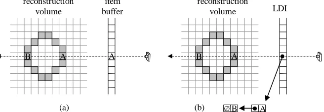
GVC determines visibility as follows. First, every voxel is assigned a unique ID. Then, an item buffer [16] is constructed for each image. An item buffer, shown in figure 1a, contains a voxel ID for every pixel in the corresponding image. While the item buffer is being computed, a distance is also stored for every pixel. A voxel V is rendered to the item buffer as follows. Scan conversion is used to find all the pixels that V projects onto. If the distance from the camera to V is less than the distance stored for the pixel, then the pixel’s stored distance and voxel ID are over-written with those of V. Thus, after a set of voxels have been rendered, each pixel will contain the ID of the closest voxel that projects onto it. This is exactly the visibility information we need.

Once valid item buffers have been computed for the images, it is then possible to compute the set vis(V) of all pixels from which the voxel V is visible. Vis(V) is computed as follows. V is projected into each image. For every pixel P in the projection of V, if P’s item buffer value equals V’s ID, then P is added to vis(V). To check the color consistency of a voxel V, we apply a consistency function consist() to vis(V) or, in other words, we compute consist(vis(V)).

reconstruction volume

item buffer

reconstruction

volume LDI

A

B A B A

B A

∅

(a) (b)

Since carving a voxel changes the visibility of the remaining uncarved voxels, and since we use item buffers to maintain visibility information, the item buffers need to be updated periodically. GVC does this by recomputing the item buffers from scratch. Since this is time consuming, we allow GVC to carve many voxels between updates. As a result, the item buffers are out-of-date much of the time and the computed set vis(V) is only guaranteed to be a subset of all the pixels from which a voxel V is visible. However, since carving is conservative, no voxels will be carved that shouldn’t be. During the final iteration of GVC, no carving occurs so the visibility information stays up-to-date. Every voxel is checked for color consistency on the final iteration so it follows that the final model is color-consistent.

As carving progresses, each voxel is in one of three categories: •it has been found to be inconsistent and has been carved;

•it is on the surface of the set of uncarved voxels and has been found to be consistent whenever it has been evaluated; or

•it is surrounded by uncarved voxels, so it is visible from no images and its consistency is undefined.

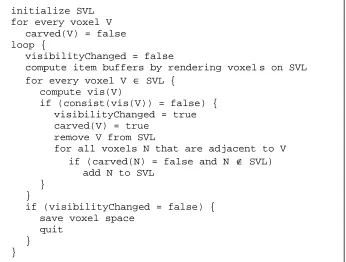
We use an array of bits, one per voxel, to record which voxels have been carved. This data structure is called carved in the pseudo-code and is initially set to false for every voxel. We maintain a data structure called the surface voxel list (SVL) to

initialize SVL for every voxel V

carved(V) = false loop {

visibilityChanged = false

compute item buffers by rendering voxel s on SVL

for every voxel V ∈ SVL {

compute vis(V)

if (consist(vis(V)) = false) { visibilityChanged = true carved(V) = true

remove V from SVL

for all voxels N that are adjacent to V

if (carved(N) = false and N ∉ SVL)

add N to SVL }

}

if (visibilityChanged = false) { save voxel space

quit } }

identify the second category of voxels. The SVL is initialized to the set of voxels that are not surrounded by other voxels. The item buffers are computed by rendering all the voxels on the SVL into them. We call voxels in the third category interior voxels. Though interior voxels are uncarved, they do not need to be rendered into the item buffers because they are not visible from any images. When a voxel is carved, adjacent interior voxels become surface voxels and are added to the SVL. To avoid adding a voxel to the SVL more than once, we need a rapid means of determining if the voxel is already on the SVL; we maintain a hash table for this purpose.

When GVC has finished, the final set of uncarved voxels may be recorded by saving the function carved() or the SVL. Pseudo-code for GVC appears in figure 2.

3.2 The GVC-LDI Algorithm

Basic GVC computes visibility in a relatively simple manner that also makes efficient use of memory. However, the visibility information is time-consuming to update. Hence, GVC updates it infrequently and it is out-of-date much of the time. This does not lead to incorrect results but it does result in inefficiency because a voxel that would be evaluated as inconsistent using all the visibility information might be evaluated as consistent using a subset of the information. Ultimately, all the information is collected but, in the meantime, voxels can remain uncarved longer than necessary and can therefore require more than an ideal number of consistency evaluations. Furthermore, GVC reevaluates the consistency of voxels on the SVL even when their visibility (and hence their consistency) has not changed since their last evaluation. By using layered depth images instead of item buffers, GVC-LDI can efficiently and immediately update the visibility information when a voxel is carved and also can precisely determine the voxels whose visibility has changed.

Unlike the item buffers used by the basic GVC method, which record at each pixel P just the closest voxel that projects onto P, the LDIs store at each pixel a list of all the surface voxels that project onto P. See figure 1b. These lists, which in the pseudo-code are called LDI(P), are sorted according to the distance of the voxel to the image’s camera. The head of LDI(P) stores the voxel closest to P, which is the same voxel an item buffer would store. Since the information stored in an item buffer is also available in an LDI, vis(V) can be computed in the same way as before. The LDIs are initialized by rendering the SVL voxels into them.

The uncarved voxels whose visibility changes when another voxel is carved come from two sources:

•They are interior voxels adjacent to the carved voxel and become surface voxels when the carved voxel becomes transparent. See figure 3a.

= SVL voxel

= voxel with changed visibility = recently carved voxel

= interior voxel

(b) carved voxels carved voxels

(a)

Fig. 3. When a voxel is carved, there are two categories of other voxels whose visibility changes: (a) interior voxels that are adjacent to the carved voxel and (b) voxels that are already on the SVL and are often distant from the carved voxel.

Voxels in the first category are trivial to identify since they are next to the carved voxel. Voxels in the second category are impossible to identify efficiently in the basic GVC method; hence, that method must repeatedly evaluate the entire SVL for color consistency. In GVC-LDI, voxels in the second category can be found easily with the aid of the LDIs; they will be the second voxel on LDI(P) for some pixel P in the projection of the carved voxel. GVC-LDI keeps a list of the SVL voxels whose visibility has changed, called the changed visibility SVL (CVSVL in the pseudo-code). These are the only voxels whose consistency must be checked. Carving is finished when the CVSVL is empty.

4

Results

We present the results of running Space Carving, GVC, and GVC-LDI on two image sets that we call “toycar” and “bench”. In particular, we present runtime statistics and provide, for side-by-side comparison, images synthesized with Space Carving and our algorithms. The experiments were run on a 440 MHz HP J5000 computer.

The toycar and bench image sets represent opposite extremes in terms of how difficult they are to reconstruct. The toycar scene is ideal for reconstruction. The seventeen 800×600-pixel images are computer-rendered and perfectly calibrated. The colors and textures make the various surfaces in the scene easy to distinguish from each other. The bench images are photographs of a natural, real-world scene. In contrast to the toycar scene, the bench scene is challenging to reconstruct for a

initialize SVL render SVL to LDIs for every voxel V

carved(V) = false copy SVL to CVSVL

while (CVSVL is not empty) { delete V from CVSVL

compute vis(V)

if (consist(vis(V)) = false) { carved(V) = true

remove V from SVL

for every pixel P in projection of V into all images { if (V is head of LDI(P))

add next voxel on LDI(P) (if any) to CVSVL delete V from LDI(P)

}

for every voxel N adjacent to V with N ∉ SVL {

N_is_visible = false

for every pixel P in projection of N to all images { add N to LDI(P)

if (N is head of LDI(P)) N_is_visible = true }

add N to SVL if (N_is_visible)

add N to CVSVL }

} }

save voxel space

number of reasons: the images are somewhat noisy, the calibration is not as good, and the scene has large areas with relatively little texture and color variation.

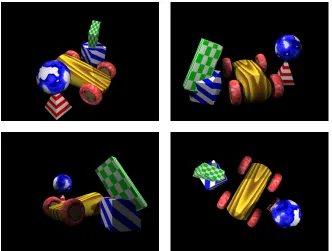
We reconstructed the toycar scene in a 167×121×101-voxel volume. Four of the input images are shown in figure 7. New views synthesized from Space Carving and GVC-LDI reconstructions are shown in figure 8. There are some holes visible along one edge of the blue-striped cube in the Space Carving reconstruction. The coloring in the Space Carving image has a noisier appearance than the GVC-LDI image.

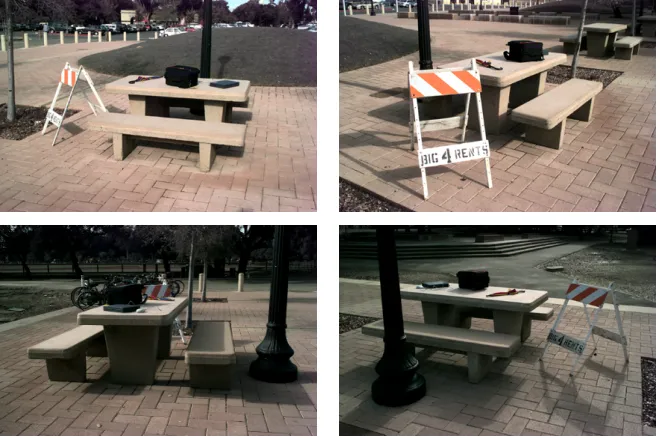
We used fifteen 765×509-pixel images of the bench scene and reconstructed a 75×71×33-voxel volume. We calibrated the images with a product called PhotoModeler Pro [17]. The points used to calibrate the images are well dispersed throughout the scene and their estimated 3D coordinates project within a maximum of 1.2 pixels of their measured locations in the images. Four of the input images are shown in figure 9. New views synthesized from Space Carving and GVC reconstructions are shown in figure 10. The Space Carving image is considerably noisier and more distorted than the GVC image.

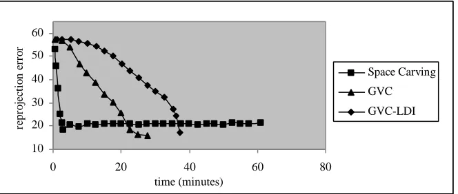
Figures 5 and 6 show the total time Space Carving, GVC, and GVC-LDI ran on the toycar and bench scenes until carving completely stopped. They also illustrate the rates at which the algorithms converged to good visual representations of the scene. We used reprojection error to estimate visual quality. Specifically, we projected models to the same viewpoint as an extra image of the actual scene, and computed the errors by comparing corresponding pixels in the projected and actual images.

Due to the widely varied color and texture in the toycar scene, the color consistency of most voxels can be correctly determined using a small fraction of the input image pixels that will ultimately be able to view the voxel in the final model. Thus, many voxels that must be carved can, in fact, be carved the first time their consistency is checked. Space Carving, with its lean data structures, checks the consistency of voxels faster (albeit, less completely) than the other algorithms and hence, as shown in figure 5, was the first to converge to a good representation of the scene. After producing a good model, Space Carving spent a long time carving a few additional voxels and was the last to completely stop carving. However, this additional carving is not productive visually. Unlike the other two algorithms,

GVC-10 20 30 40 50 60

0 20 40 60 80

time (minutes)

reprojection error

Space Carving

GVC

GVC-LDI

LDI spends extra time to find all the pixels that can view a voxel when checking a voxel’s consistency. In the toycar scene, this precision was not helpful and caused GVC-LDI to converge the slowest to a good visual model. Ultimately, GVC and GVC-LDI reconstructed models with somewhat lower reprojection error than Space Carving.

The convergence characteristics of the algorithms were different for the bench scene, as shown in figure 6. The color and texture of this scene make reconstruction difficult but are probably typical of the real-world scenes that we are most interested in reconstructing. In contrast to the toycar scene, many voxels in the bench scene are very close to the color-consistency threshold. Hence, many voxels that must be carved cannot be shown to be inconsistent until they become visible from a large number of pixels. Initially, all three algorithms converge at roughly the same rate. Then Space Carving stops improving in reprojection error but continues slow carving. GVC and GVC-LDI produce models of similar quality, both with considerably less error than Space Carving. After an initial period of relatively rapid carving, GVC then slows to a carving rate of several hundred voxels per iteration. Because, on each of these iterations, GVC recalculates all its item buffers and checks the consistency of thousands of voxels, it takes GVC a long time to converge to a color-consistent model. For the bench scene, the efficiency of GVC-LDI’s relatively complex data structures more than compensates for the time needed to maintain them. Because GVC-LDI finds all the pixels from which a voxel is visible, it can carve many voxels sooner, when the model is less refined, than the other algorithms. Furthermore, after

30 40 50 60 70 80 90 100

0 10 20 30 40 50 60

time (minutes)

reprojection error

Space Carving GVC GVC-LDI

Fig. 6. Convergence of the algorithms while reconstructing the “bench” scene.

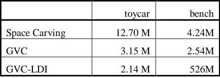
toycar bench

Space Carving 12.70 M 4.24M

GVC 3.15 M 2.54M

GVC-LDI 2.14 M 526M

carving a voxel, GVC-LDI only reevaluates the few other voxels whose visibility has changed. Consequently, GVC-LDI is faster than GVC by a large margin. On both the toycar and the bench scene, GVC-LDI used the fewer color consistency checks than the other algorithms, as shown in table 1.

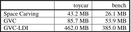
All three algorithms keep copies of the input images in memory. The images dominate the memory usage for Space Carving. GVC uses an equal amount of memory for the images and the item buffers and, consequently, uses about twice as much memory as Space Carving, as shown in table 2. The LDIs dominate the memory usage in GVC-LDI and consume an amount of memory roughly proportional to the number of image pixels times the depth complexity of the scene. The table shows that GVC-LDI uses considerably more memory than the other two algorithms. Memory consumed by the carve and SVL data structures is relatively insignificant and, therefore, the voxel resolution has little bearing on the memory requirements for GVC and GVC-LDI.

toycar bench

Space Carving 43.2 MB 26.1 MB

GVC 85.7 MB 53.9 MB

GVC-LDI 462.0 MB 385.0 MB

Table 2. The memory used by the algorithms while reconstructing the “toycar” and “bench” scenes.

Kutulakos and Seitz have shown that for a given image set and monotonic consistency function, there is a unique maximal color-consistent set of voxels, which they call V*. Since GVC and GVC-LDI do not stop carving until the remaining uncarved voxels are all color-consistent and since they never carve consistent voxels, we expect them to produce identical results, namely V*, when used with a monotonic consistency function. However, monotonic consistency functions can be hard to construct. An obvious choice for consist(S) would take the maximum difference between the colors of any two pixels in S. However, using distance in the RGB cube as a difference measure, this function is O(n2) on the size of S and has poor immunity to noise and high-frequency color variation. We actually use standard deviation for the consistency function and it is not monotonic. Consequently, GVC and GVC-LDI generally produce models that are different but similar in quality.

5

Future Work

into the statistics for the correct voxels. Besides reducing the amount of rendering, this approach has three other benefits. First, we will not need the item buffer again after processing an image. Thus, the same memory can be used for all the item buffers, reducing the memory requirement relative to our current implementation. Second, the rendering that is still required can be easily accelerated with a hardware graphics processor. Third, the processing that must be performed on one image is independent of the processing for the rest of the images. Thus, on one iteration, each image can be rendered on a separate, parallel processor.

We believe LDIs have great potential for use in voxel-based reconstruction algorithms. A hybrid algorithm could make the memory requirements for LDIs more practical. In such an approach, an algorithm like GVC would be used to find a rough model. GVC runs most efficiently during its earliest iterations, when many voxels can be carved on each iteration. Once a rough model has been obtained, GVC-LDI could be used to refine local regions of the model. The rough model should be sufficient to find the subset of images from which the region is visible. The subset is likely to be considerably smaller than the original set, so the memory requirements for the LDIs should be much smaller. GVC-LDI would run until the model of the region converges to color-consistency. If the convergence is slow, GVC-LDI should be much faster than GVC.

The algorithms described in this paper find a set of voxels whose color inconsistency falls below a threshold. It would be preferable to have an algorithm that would attempt to minimize color inconsistency to find the model that is most consistent with the input images. We have already mentioned that LDIs can efficiently maintain visibility information when voxels are removed from the model, i.e. carved, but, in fact, they can also be used to efficiently maintain visibility information when voxels are moved or added to the model. Thus, LDIs could be a key element in an algorithm that would add, delete, and move voxels in a model to minimize its reprojection error.

6

Conclusion

Acknowledgements

We would like to thank Steve Seitz for numerous discussions. We are indebted to Mark Livingston, who performed the difficult task of calibrating the bench image set. We are grateful for the support of our management, especially Fred Kitson.

References

1. S. Seitz, Charles R. Dyer, “Photorealistic Scene Reconstruction by Voxel Coloring”,

Proceedings of Computer Vision and Pattern Recognition Conference, 1997, pp. 1067-1073.

2. K. N. Kutulakos and S. M. Seitz, “What Do N Photographs Tell Us about 3D Shape?”

TR680, Computer Science Dept. U. Rochester, January 1998.

3. S. Seitz, Charles R. Dyer, “View Morphing”, Proceedings of SIGGRAPH 1996, pp. 21-30. 4. M. Levoy and P. Hanrahan, “Light Field Rendering”, Proceedings of SIGGRAPH 1996, pp.

31-42.

5. S. Gortler, R. Grzeszczuk, R. Szeliski, M. Cohen, “The Lumigraph”, Proceedings of SIGGRAPH 1996, pp. 43-54.

6. H. Shum, H. Li-Wei, “Rendering with Concentric Mosaics”, Proceedings of SIGGRAPH 99, pp. 299-306.

7. W. E. L. Grimson, “Computational experiments with a feature based stereo algorithm”,

IEEE Transactions on Pattern Analysis and Machine Intelligence, vol. 7, no. 1, January 1985, pp. 17-34.

8. M. Okutomi, T. Kanade, “A Multi-baseline Stereo”, IEEE Transactions on Pattern Analysis and Machine Intelligence, vol. 15, No. 4, April 1993, pp. 353-363.

9. P. J. Narayanan, P. Rander, T. Kanade, “Constucting Virtual Worlds Using Dense Stereo”,

IEEE International Conference on Computer Vision, 1998, pp. 3-10.

10. S. Roy, I. Cox, “A Maximum-Flow Formulation of the N-camera Stereo Correspondence Problem”, IEEE International Conference on Computer Vision, 1998, pp. 492-499. 11. R. Szeliski, P. Golland, “Stereo Matching with Transparency and Matting”, IEEE

International Conference on Computer Vision, 1998, pp. 517-524.

12. O. Faugeras, R. Keriven, “Complete Dense Stereovision using Level Set Methods”, Fifth European Conference on Computer Vision, 1998.

13. H. Saito, T. Kanade, “Shape Reconstruction in Projective Grid Space from Large Number of Images”, Proceedings of Computer Vision and Pattern Recognition Conference, 1999, volume 2, pp. 49-54.

14. N. Max, “Hierarchical Rendering of Trees from Precomputed Multi-Layer Z-Buffers”,

Eurographics Rendering Workshop 1996, pp 165-174.

15. J. Shade, S. Gortler, L. He, R. Szeliski, “Layered Depth Images”, Proceedings of SIGGRAPH 98, pp. 231-242.

16. H. Weghorst, G. Hooper, D. P. Greenberg, “Improving Computational Methods for Ray Tracing”, ACM Transactions on Graphics, 3(1), January 1984, pp. 52-69.

Fig. 7. Four of the seventeen images of the toycar scene.

Fig. 9. Four of the fifteen input images of the bench scene.