Infectiousness
Alexander V. Mantzaris and Desmond J. Higham
Abstract Using real, time-dependent social interaction data, we look at correla-tions between some recently proposed dynamic centrality measures and summaries from large-scale epidemic simulations. The evolving network arises from email ex-changes. The centrality measures, which are relatively inexpensive to compute, as-sign rankings to individual nodes based on their ability to broadcast information over the dynamic topology. We compare these with node rankings based on infectious-ness that arise when a full stochastic SI simulation is performed over the dynamic network. More precisely, we look at the proportion of the network that a node is able to infect over a fixed time period, and the length of time that it takes for a node to in-fect half the network. We find that the dynamic centrality measures are an excellent, and inexpensive, proxy for the full simulation-based measures.
1 Background and Motivation
In many social interactions, the timing of the connections is vital. Suppose A meets B today and B meets C tomorrow. This makes it possible for a message, or a disease, to pass from A to B, but not from C to A. Further, the more active B happens to be tomorrow, the more potential there is for today’s A-B link to have a downstream ef-fect. Several authors have pointed out the need to account for topological dynamics when considering disease propagation. The work in [15] considers the stages that sexually transmitted diseases (STDs) pass through when infecting subpopulations of a network, and shows that the timing in the connectivity between individuals plays a crucial role. In [10] a disease is simulated with an SI model (as we use here) and an SIR alternative, over contact networks relating to high-end prostitution. Both a static and a temporal view of the interaction data is used, and the results show that temporal effects play a key role. Epidemic simulations over temporal connectivity
Department of Mathematics and Statistics, University of Strathclyde, Glasgow, UK e-mail: [email protected]
data are also used in [7] to explore vaccination strategies. Similarly, the spread of computer malware over temporal networks is considered in [12, 11], and strategies developed for the immunisation of key nodes. The SI framework is used in [2] to characterise the global structure of a temporal network.
From a network science perspective, it is natural to seek genericcentrality mea-sures that rank individual nodes according to their “importance.” In the case of static network topology, there is a wealth of such measures, most of which can be traced back to the social network analysis community [4]. Devising centrality measures that apply to time-dependent networks is a more recent pursuit. The work of [14] used a shortest-path-counting approach to measure the closeness/betweeness of nodes in a time varying graph. The alternative walk-counting approach in [5] was based on a direct generalization of Katz centrality [6] to the case of time-dependent networks. A key message from [13] and [8] is that centrality measures based on a static, aggregate summary of the network will not adequately reflect the hierarchy of importance.
The question that we address in this work is
given a time-dependent network, can suitable centrality measures provide useful informa-tion about the spread of epidemics?
The question is motivated by the fact that centrality measures are typically much cheaper to compute than large-scale stochastic simulations. For this reason, we focus on the dynamic communicability approach in [5] where we can deal with all nodes simultaneously by solving a sparse linear system at each time step (that is, findingx
in a matrix-vector system of the formAx=b, whereAhas the same sparsity as the current network adjacency matrix).
In the next section we give details of the computational tasks and the data set used. Sections 3 and 4 describe the data and results, and we finish with a discussion in Section 5.
2 Methodology
We consider a fixed set ofN nodes whose connections are recorded at an equally spaced set of time pointst0<t1<· · ·<tM. The network at each time point is
undirected and unweighted, with no self loops. So, at timetk, we can record the state of the network in the adjacency matrixA[k]∈RN×N. HereA[k]
i j=1 if node
ihas a link to node jat timetkand
A[k]
i j=0 otherwise.
The epidemic simulations are peformed in a stochastic SI framework. At each time point a node is either susceptible (S) or infectious (I). Once made infectious, a node cannot return to the susceptible state. We begin, att0, by infecting a single
node. Generally, to determine the status of the nodes at timetk+1, we use the
fol-lowing rule: for each node that was in the infectious state at timetk, we consider
susceptible state, then it is moved into the infectious state with independent proba-bilityβ. More loosely, an infectious node has a fixed probabilityβ of transmitting the infection to each of itscurrentcontacts.
We measure the virulence of a node in two separate ways. After starting the infection at this node, we compute
(a) the proportion of the network infected at the final time,tM,
(b) the number of time points required to infect at least half of the network. To understand the centrality measures from [5], we need to introduce the concept of adynamic walk of length w from node i to node j: this is simply any traversal fromito jalongwedges that respects the arrow of time (i.e. having used an edge at timetr, the next edge that we use must exist at timetr or later). The ability of
nodeito broadcast information to node jmay then be measured as the total number of dynamic walks fromito j, where a walk of lengthwis downweighted by the factorαw. Hereα∈(0,1)is a fixed parameter that reduces the influence of longer walks. In the case of a single time point, this measure reduces to the classical Katz centrality [6], which may be computed through the matrix resolvent,(I−αA)−1. Generalizing to multiple time points in this way, we arrive at the expression
Q=I−αA[0]
−1
I−αA[1]
−1
. . .I−αA[M]
−1
, (1)
whereQi jmeasures how well nodeican broadcast information to nodej. To obtain
a single coefficient for nodeiwe sum over all nodes in the network to obtain the
broadcast centrality. In practice, since we plan to use this measure to rank the nodes, it is reasonable to normalize, which avoids numerical underflow/overflow, leading to the iteration
ˆ
Q[k]=
ˆ
Q[k−1]I− αA[k]
−1 ˆ
Q[k−1] I−αA[k]−1
, (2)
fork=0, . . . ,M, with ˆQ[−1]=Iandk · krepresenting the Euclidean matrix norm. The broadcast centrality for nodeiis then given by∑Nj=1
ˆ
Q[k] i j.
Just as in the original Katz version, this centrality measure involves a parameter,
α. In order for the matrix inverses to exist, we requireαto be less than
α?:= min 0≤k≤M ρ A[k] −1 ,
whereρ(·)denotes the spectral radius. Tests in [5] indicated that the results are not
3 Data
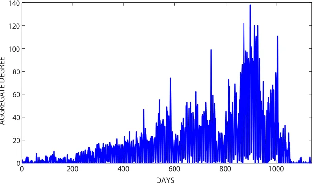
We perform the tests on real social interaction data that records email exchanges between former Enron employees [3, 9]. There areN=151 individuals, and we summarize activity into daily time slices: an undirected edge betweeni and j in-dicates that at least one email (including cc and bcc) passed between the two individuals. Figure 1 shows a plot of the static aggregate degree each day for all the nodes. Because the start date is arbitrary, we smooth out its influence by repeating
0 200 400 600 800 1000
0 20 40 60 80 100 120 140
DAYS
AGGREGATE DEGREE
Fig. 1 The static aggregate degree each day for all of the nodes (Enron employees).
computations over a sliding window that covers half the overall period; that is, 568 of the 1036 consecutive days. So the first window runs from day 1 to day 568, the second window runs from day 2 to day 569, and so on. In this manner, we create 568 distinct evolving networks, each involvingM+1=568 consecutive days. Results are averaged over all windows.
For each of the 568 windows, we compute the broadcast centralities and, with each node in turn as a starting point for infection, perform one SI simulation. In practice we found that computing the broadcast centralities was typically an order of magnitude faster than computingN=151 paths of the SI model, one from each starting state.
[image:4.612.139.462.218.406.2]Table 1 Symbols for company position
President hexagram
CEO pentagram
Executive pentagram
Legal diamond
VicePresident hexagram
DirectorofTrading square ManagingDirector upward triangle
Manager right facing triangle Director left facing triangle
InHouseLawyer diamond
Trader square
Employee plus
Secretary circle
all others small dot
Table 2 Correlation coefficients relating to Figures 3, 7 and 11 for broadcast versus proportion of
the network infected.
β Pearson Kendall Tau Spearman
0.2 0.85 0.70 0.88
0.5 0.88 0.82 0.94
1.0 0.94 0.81 0.94
The Enron data set also provides the positions of most employees within the com-pany. For completeness, we display this information in our figures. Table 1 indicates the symbols that we use. However, in the results that follow there does not appear to be any clear pattern based on these semantic labels.
4 Results
The SI simulations were repeated for three different choices of the infection proba-bility,β. In each case, we provide two dimensional scatter plots (one point for each
node) that compare, in a pair-wise fashion, (a) the proportion of the network infected at the final time point, (b) the time taken to infect 50% of the network, and (c) the natural logarithm of the broadcast centrality. The corresponding Pearson, Kendall Tau and Spearman correlation coeficients for the (a)-(c) pair are reported in Table 2. We also scatter plot the aggregate degree—that is, the total number of edges involving the node over all time points—against the proportion of the network in-fected.
4.1 Infection rate
β
=
0.2
results
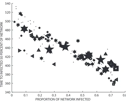
Forβ=0.2, Figure 2 focuses on the SI model and compares the infected proportion against the time to infect 50%. These are seen to have a strong negative correla-tion, and hence, in terms of ranking the nodes by infectiousness, they are broadly comparable.
0 0.1 0.2 0.3 0.4 0.5 0.6 0.7 0.8 340
360 380 400 420 440 460 480 500 520 540
PROPORTION OF NETWORK INFECTED
TIME TO INFECTED 50 PERCENT OF NETWORK
Fig. 2 Infected proportion versus time for 50% of the network to be infected forβ=0.2.
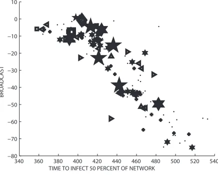
The broadcast centrality is compared with the infected proportion in Figure 3 and with the time to infect 50% in Figure 4. In both cases, we see strong correlations.
In Figure 5 we show the aggregate degree against the infection level. Although most of the very high degree nodes are typically strong infectors, the relationship is far from linear and breaks down at the lower levels. We also emphasize that the integer-valued nature of nodal degree makes it liable to produce more ties when used to rank nodes.
4.2 Infection rate
β
=
0.5
results
We now repeat the experiments from subsection 4.1 with a stronger infection rate of
β =0.5.
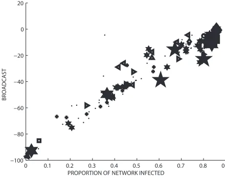
[image:6.612.187.404.200.377.2]0 0.1 0.2 0.3 0.4 0.5 0.6 0.7 0.8 −100
−80 −60 −40 −20 0 20
PROPORTION OF NETWORK INFECTED
BROADCAST
Fig. 3 Broadcast centrality versus infected proportion forβ=0.2.
340 360 380 400 420 440 460 480 500 520 540 −80
−70 −60 −50 −40 −30 −20 −10 0 10
TIME TO INFECT 50 PERCENT OF NETWORK
BROADCAST
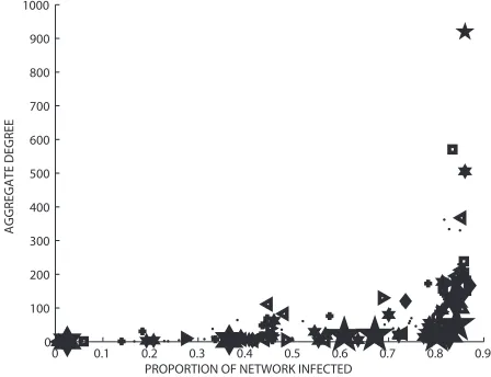
[image:7.612.184.400.105.282.2] [image:7.612.188.406.334.509.2]0 0.1 0.2 0.3 0.4 0.5 0.6 0.7 0.8 0
100 200 300 400 500 600 700 800 900 1000
PROPORTION OF NETWORK INFECTED
AGGREGATE DEGREE
Fig. 5 Average degree versus infected percentage forβ=0.2.
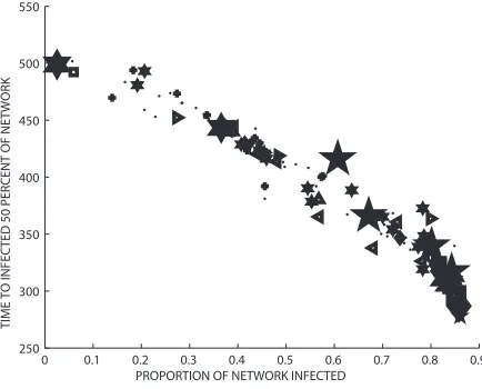
0 0.1 0.2 0.3 0.4 0.5 0.6 0.7 0.8 0.9
250 300 350 400 450 500 550
PROPORTION OF NETWORK INFECTED
TIME TO INFECTED 50 PERCENT OF NETWORK
[image:8.612.179.403.95.281.2] [image:8.612.187.404.333.508.2]Figures 7 and 8 compare the broadcast centrality with infected proportion and time to infect 50%, respectively. The performance of the broadcast measure as a proxy seems to improve slightly over theβ=0.2 case. This is confirmed in Table 2 in terms of the three correlation coefficients.
0 0.1 0.2 0.3 0.4 0.5 0.6 0.7 0.8 0.9
−100 −80 −60 −40 −20 0 20
PROPORTION OF NETWORK INFECTED
BROADCAST
Fig. 7 Broadcast centrality versus infected proportion forβ=0.5.
250 300 350 400 450 500 550
−100 −80 −60 −40 −20 0 20
TIME TO INFECT 50 PERCENT OF NETWORK
BROADCAST
[image:9.612.182.402.173.348.2] [image:9.612.185.408.422.601.2]Figure 9 shows the aggregate degree against infected proportion and the effect observed forβ=0.2 is now further exaggerated.
0 0.1 0.2 0.3 0.4 0.5 0.6 0.7 0.8 0.9 0
100 200 300 400 500 600 700 800 900 1000
PROPORTION OF NETWORK INFECTED
AGGREGATE DEGREE
Fig. 9 Average degree versus infected proportion forβ=0.5.
4.3 Infection rate
β
=
1.0
results
The final set of tests usesβ=1.0 in the SI model. In this case the disease
transmis-sion is no longer stochastic.
[image:10.612.182.406.152.324.2]0.1 0.2 0.3 0.4 0.5 0.6 0.7 0.8 0.9 200
250 300 350 400 450 500 550
PROPORTION OF NETWORK INFECTED
[image:11.612.187.403.106.283.2]TIME TO INFECTED 50 PERCENT OF NETWORK
Fig. 10 Infected percentage versus time for 50% of the network to be infected forβ=1.0.
0 0.1 0.2 0.3 0.4 0.5 0.6 0.7 0.8 0.9 −100
−80 −60 −40 −20 0 20
PROPORTION OF NETWORK INFECTED
BROADCAST
[image:11.612.183.405.334.508.2]200 250 300 350 400 450 500 550 −100
−80 −60 −40 −20 0 20
TIME TO INFECT 50 PERCENT OF NETWORK
[image:12.612.185.408.94.281.2]BROADCAST
Fig. 12 Broadcast centrality versus time to reach 50% network infection forβ=1.0.
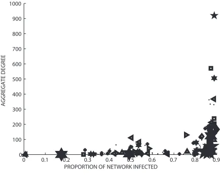
Finally, Figure 13 shows again that the aggregate degree is a poor predictor of the infected network proportion.
0 0.1 0.2 0.3 0.4 0.5 0.6 0.7 0.8 0.9 0
100 200 300 400 500 600 700 800 900 1000
PROPORTION OF NETWORK INFECTED
AGGREGATE DEGREE
[image:12.612.183.406.388.566.2]5 Discussion
We are concerned here with quantifying properties of a time-dependent interaction network in terms of epidemic spread. Our results indicate that ranking nodes accord-ing to their broadcast centrality from [5] can operate as an accurate, and relatively inexpensive, proxy for more detailed rankings of their ability to spread infection based on averaging over microscale simulations. In particular, the results were in-sensitive to infection probability in the microscale model. By contrast, simply judg-ing a node by its overall bandwidth does not provide a useful picture.
There are many avenues for extending this type of study. For example:
• Further investigation is needed to test whether improvements will arise from fine tuning the Katz-style downweighting parameterαused in the broadcast central-ity measure, as a function of the infection probabilcentral-ity,β.
• Other types of interaction data could be used to generate the underlying dynamic topology.
• The accompanyingreceive centralitymeasure from [5] can be tested as a proxy for the vulnerability of a node to infection.
• More complex compartmental epidemic models could be investigated, including SIS and SIR. In this case, our intuition is that the straightforward dynamic walk counting approach of [5] will be less successful, and hence new classes of time-respecting network centrality measures will be required.
• In addition to local node-based information, global summaries, such as an ap-propriate, dynamic, version of the basic reproduction number,R0, could be
com-pared with network features. A study of this type has recently been performed for the case of a static network in [1].
Acknowledgment
This work was supported by the Engineering and Physical Sciences Research Council and the Research Councils UK Digital Economy Programme, under grant EP/I016058/1. DJH was also supported by a Fellowship from the Leverhulme Trust.
References
1. Ames, G., George, D., Hampson, C., Kanarek, A., McBee, C., Lockwood, D., Achter, J., Webb, C.: Using network properties to predict disease dynamics on human contact networks. Proc Biol Sci.278(1724), 3544–50 (2011)
2. Barrat, A., Cattuto, C.: Temporal networks of face-to-face human interactions. In: P. Holme, J. Saram¨aki (eds.) Temporal Networks. Springer (2013)
3. Carvalho, V.R., W.Cohen, W.: Recommending recipients in the Enron email corpus. Tech. Rep. CMU-LTI-07-005, Carnegie Mellon University (2007)
5. Grindrod, P., Higham, D.J., Parsons, M.C., Estrada, E.: Communicability across evolving net-works. Physical Review E83, 046,120 (2011)
6. Katz, L.: A new index derived from sociometric data analysis. Psychometrika18, 39–43 (1953)
7. Lee, S., Rocha, L.E.C., Liljeros, F., Holme, P.: Exploiting temporal network structures of human interaction to effectively immunize populations. PLoS ONE7(2012)
8. Mantzaris, A.V., Higham, D.J.: Dynamic communicators. to appear in European Journal of Applied Mathematics (2012)
9. Nicosia, V., Tang, J., Mascolo, C., Musolesi, M., Russo, G., Latora, V.: Graph metrics for temporal networks. In: P. Holme, J. Saram¨aki (eds.) Temporal Networks. Springer (2013) 10. Rocha, L.E.C., Liljeros, F., Holme, P.: Simulated epidemics in an empirical spatiotemporal
network of 50,185 sexual contacts. PLoS Comput Biol7(2011)
11. Tang, J., Leontiadis, I., Scellato, S., Nicosia, V., Mascolo, C., Musolesi, M., Latora, V.: Ap-plications of temporal graph metrics to real-world networks. In: P. Holme, J. Saram¨aki (eds.) Temporal Networks. Springer (2013)
12. Tang, J., Mascolo, C., Musolesi, M., Latora, V.: Exploiting temporal complex network metrics in mobile malware containment. In: Proceedings of IEEE 12th International Symposium on a World of Wireless Mobile and Multimedia Networks (WOWMOM) (2011)
13. Tang, J., Musolesi, M., Mascolo, C., Latora, V., Nicosia, V.: Analysing information flows and key mediators through temporal centrality metrics. In: SNS ’10: Proceedings of the 3rd Workshop on Social Network Systems, pp. 1–6. ACM, New York, NY, USA (2010). DOI http://doi.acm.org/10.1145/1852658.1852661
14. Tang, J., Scellato, S., Musolesi, M., Mascolo, C., Latora, V.: Small-world behavior in time-varying graphs. Physical Review E.81(2010)