Evolution in Knockout Contests: the Variable Strategy Case

City, University of London Institutional Repository

Citation:

Broom, M., Cannings, C. and Vickers, G. T. (2000). Evolution in Knockout Contests: the Variable Strategy Case. Selection, 1, pp. 5-21.

This is the unspecified version of the paper.

This version of the publication may differ from the final published

version.

Permanent repository link:

http://openaccess.city.ac.uk/990/

Link to published version:

Copyright and reuse: City Research Online aims to make research

outputs of City, University of London available to a wider audience.

Copyright and Moral Rights remain with the author(s) and/or copyright

holders. URLs from City Research Online may be freely distributed and

linked to.

City Research Online: http://openaccess.city.ac.uk/ [email protected]

Evolution in Knockout Contests: The Variable Strategy Case

M. BROOM1_{*, C. CANNINGS}2_{and G. T. VICKERS}3

1_{Centre for Statistics and Stochastic Modelling, School of Mathematical Sciences,}

The University of Sussex, Sussex, UK

2_{Division of Molecular and Genetic Medicine, School of Medicine, Royal Hallamshire Hospital,}

The University of Sheffield, Sheffield, UK

3_{Department of Applied Mathematics, School of Mathematics and Statistics,}

The University of Sheffield, Sheffield, UK

(Received: 11 February 2000, Accepted in revised form: 16 June 2000)

In a previous paper we introduced a model of a multi-player conflict in the form of a knockout tournament. Groups of individuals resolved their disputes in a tournament in which in each round the remaining contestants formed pairs who competed against each other: in such a contest between two individuals using behavioursxandythere was a probability that each would win, and a cost incurred by the loser, both of which depended onxandy. The winner pro-gressed to the next round of the tournament and the loser was eliminated; a player received a reward which depended on how far that individual progressed. Individuals were constrained to adopt a fixed play throughout the tournament. In this paper we extend the model by allowing individuals to vary their choice of behaviour from round to round. The complexity of such systems is investigated and illustrated by both special cases and numerical examples. It is shown that in this case behaviour is very different to the fixed strategy case.

Keywords: Multi-player games, dominance, ESS, knockout tournament, local strategy

1. Introduction

Game theory has a relatively short but valuable his-tory in modelling the natural world, especially in the area of animal conflicts. It has provided explana-tions for apparently paradoxical situaexplana-tions, such as the practice of heavily armed animals engaging only in ritualistic contests (Maynard Smith, 1982) and the tendency of (especially male) animals to develop ex-tremely costly signals to acquire mates (Grafen, 1990a, b). The concept of an Evolutionarily Stable Strategy (ESS), introduced by Maynard Smith and Price (1973) has been especially useful, and has been central to a large body of literature; some im-portant examples being (Haigh 1975; Bishop and Cannings, 1976; Maynard Smith, 1982; Cressman, 1992; Hofbauer and Sigmund, 1998). Most of this work has concentrated on games between only two players.

Game theory has its roots in economics originat-ing with von Neumann and Morgenstern (1944) (also see Alexrod and Hamilton, 1981 and Binmore, 1992), and multi-player games have always been central to its theory. See Luce and Raiffa (1957) for a general discussion, and a description of its applica-tion to voting schemes. The authors have recently written a series of papers developing multi-player models of biological situations (Broom et al., 1996, 1997a, b, 2000). If it is supposed that individuals

come together in groups of sizenand that each

indi-vidual freely selects its play, then it is necessary to specify the payoff of each possible play against ev-ery possible combination of plays chosen by the

other (n– 1) individuals in the group. In Broom et al.

(1997b) this specification was made tractable by the choice of the particular structure imposed, namely symmetric finite contests [also see Cannings and Whittaker (1994) for a similar treatment of the multi-player war of attrition]. The others only allow ‘fights’ between pairs, but have these fights embed-ded within a structure [for another example, see Mesterton-Gibbons and Dugatkin (1995) who adopted a round-robin approach in modelling a dominance hierarchy]. This paper, following on

* M. Broom is also a member of the Centre for the Study of Evolution at the University Sussex.

from Broom et al. (2000), adopts the latter approach, modelling a multi-player conflict as a set of pairwise games in a knockout tournament format. Of course this will not reflect the precise behaviour of any real population but will capture certain aspects of impor-tance. For a more detailed rationale, see Broom et al. (2000).

There now follows a reiteration of some two-player game theory which is of relevance to work later in the paper.

In the classical two-player conflict models it is assumed that individuals compete in pairwise games for some reward, food or mates perhaps. In the sym-metric version, which is our concern here, all mem-bers of the population are indistinguishable and each individual is equally likely to meet each other indi-vidual. There is a set S of choices available to each player to play in a particular game, referred to as pure strategies. Each contest results in a payoff to each of the protagonists which is specified by some

a(x, y), the payoff to an individual who plays

strat-egyxwhen opposed by an individual who playsy;x,

y∈S.

Individuals do not need to play the same pure

strategy every time, they can play amixed strategy

i.e. playxwith probability (or probability density)px

for each ofx∈S. The payoffs are presumed to be

ad-ditive over both the first and second argument, so that, for example, if S = (S1,…,Sn), the payoff to an

individual playing p against an individual playing q,

which is written asE[p, q], is given by

E[ ,p q]=

∑

a p qij i j =p AqT

where A is the matrix whose (i, j)-element is a(Si,

Sj).

p is an ESS of A if and only if, for all q¹p,

(i) E[ , ]p p ≥E[ , ]q p and

(ii) ifE[ , ]p p =E[ , ]q p thenE[ , ]p q >E[ , ]q q.

See Maynard Smith (1982) or Haigh (1975) for a more detailed explanation.

The vector p is aNash equilibriumif it satisfies

condition (i) above against all q≠p, but not

neces-sarily condition (ii) (see Hofbauer and Sigmund,

1998). The concept of an ESS can easily be extended to the multi-player case (see Palm, 1984 and Broom et al., 1997b).

The model developed in Broom et al. (2000) pro-vided a number of predictions. For the case where the pairwise games were the classical Hawk–Dove game the more players, and hence the more rounds that were played, the smaller the frequency of the aggressive Hawk strategy amongst the population. However, the frequency of individuals playing Hawk in a particular contest could rise, since Hawk individuals were more likely to progress to the later rounds. In general the structure of the tournament had a large bearing on the overall level of aggres-sion, which could be both less than or greater than that for independent games (and the difference could be fairly large). The model also predicted a relation-ship between the level of aggression in a population and the degree to which rewards are unevenly split

amongst individuals, the concept of reproductive

skewfirst developed in Vehrencamp (1983).

It was shown that there may be many ESSs for the type of knockout model described in Broom et al. (2000), although if there are only two options avail-able it is impossible to have no ESS. It was shown that for the Hawk–Dove case, there is a unique ESS, which can be evaluated numerically via a formula given in Broom et al. (2000).

1.1. The structure of knockout games

A knockout contest is a multi-player game which is composed of a number of pairwise games. Initially

there are 2n _{players each of whom plays another}

player in a pairwise game in which there is a ‘win-ner’. The winners are then repaired in the next round and this continues until there is one overall winner. Players receive a reward according to which round they were eliminated from the competition, usually increasing with the number of rounds the player sur-vives. Opponents in each round are chosen at ran-dom, and we assume here that players do not differ in any aspect which affects their performance, other than the selection of strategies. Thus the organisa-tion is similar to many human competiorganisa-tions, such as the Wimbledon Lawn Tennis Championships, al-though at Wimbledon individuals are not of equal quality and there is a seeding system which keeps apart the stronger players in the early rounds.

of individuals into a (relatively small) collection of pairwise games, and it has one of the simplest con-ceivable structures of pairwise games where every individual starts from an identical position. How-ever, as we shall see, interesting phenomena can be observed from groups of as few as 4 players. The disadvantage is that it is not realistic for a large group of animals to form themselves into fighting pairs in such an ordered way, although it is not un-reasonable to think that a structure approximating to the knockout model might occur in some circum-stances. In addition large groups that are stable will have already formed a hierarchy, and groups re-forming may well have a memory of other individu-als (see, for example, Barnard and Burk, 1979). So the model may only be useful in considering groups which form for the first time.

Initially there are 2n_{players who play a pairwise}

game with one opponent such that there is a ‘winner’ and a ‘loser’. The loser is eliminated from the com-petition and the winner enters the next round, where

the process is repeated with 2n–1_{players. This}

con-tinues until the final round with only two players.

Define roundkas the round with 2k_players

remain-ing, i.e. the players start in round n, and the final

round is round 1. This is the opposite to the round numbering system used in most sporting contests, but is mathematically more convenient. Losers in

round k gain the rewardV_k, the overall winner

re-ceivingV₀. It is assumed that V_k³ V_{k + 1}(k = 0,…, n–1).

The pairwise games which are played in the knockout contest could be any game which has a winner and a loser. As in Broom et al. (2000), we consider a very simple game in this paper. The pairwise game which is played in each round is de-fined as follows:

Suppose that in each round there are availablem

strategies labelledO₁, …, O_m.These shall henceforth

be referred to asoptions. Terms such asmixed

op-tionwill be used. The termstrategywill be reserved

for the overall strategy specifying which option is to be used for each round should the player progress to that round. This specification may be probabilistic, comprising all the options from each round. Let the probability that aO_i-player beats aO_j-player be ½ +

∆ij, so that∆ij+∆ji= 0 and∆ii= 0. In addition if aOi

-player loses to aO_j-player it incurs a costc_ij (a

re-ward–c_ij), which might correspond to an injury, or

loss of time or energy.

In Broom et al. (2000) each player used the same option in each round. In this paper players may vary their option from round to round. Note that the two cases can be thought of as the two extreme cases out of a set of possible types of game (see Broom et al.,

2000). Our conflicts each involve 2n_{individuals and}

we envision a population which has a large

(essen-tially infinite) set of such conflicts. The set of 2n

players are selected at random from the infinite pop-ulation of players.

2. A variable strategy

In this paper we allow players to change their option from round to round. As opposed to the fixed strat-egy case, and as in any two-player conflict, we do not need to differentiate in any round as to whether individuals are playing pure or mixed options; it is only the overall population play which matters. We find a recurrence relation for the evolutionary stable

play in roundk conditional on all lower numbered

rounds (i.e. rounds later in the competition). The term Evolutionarily Stable Option (ESO) is coined for such play (formally defined in Section 2.2) and we show that a collection of ESOs for each round forms a Nash equilibrium. In Sections 2.3–2.6 we consider the 2 and 3 option cases in more detail.

The type of contest that we consider has a lot in

common with extensive two-person games

de-scribed by Selten (1983) (see also Van Damme, 1991). Both games use a dynamic programming ap-proach, finding optimal play at any stage of the game conditional upon optimal play at later stages.

Selten (1983) uses the termlocal strategyfor what

we call an option and any collection of local

strate-gies is referred to as abehaviour strategy. In case of

2.1. The equivalence of different strategy combinations

Fornrounds andmoptions, which we labelO₁, …,

O_m, there aremn_{pure strategies (a selection of an} op-tion for each round). However, the same populaop-tion structure can be obtained from different mixtures of these.

Consider the case wherem = n= 2. The four

pos-sible pure strategies areS₁₁, S₁₂, S₂₁andS₂₂(the first subscript is the option played in round 1, the second

in round 2). Let the proportions ofS_ijat the start be

r_ij, so that

r₁₁+ r₁₂+ r₂₁+ r₂₂= 1

Further, let the proportion ofO1-players in round 2

bep2= r11+ r21, and the proportion in round 1 bep₁.

The probability of a O₁-player reaching round 1 is

½ +∆(1 –p₂) and for aO₂-player it is ½ –∆p2, where

∆=∆12. Therefore

p₁= [1 + 2∆(1 –p2)]r11+ (1 – 2∆p2)r12.

Together with the equationp₂= r₁₁+ r₂₁, this gives

two equations in three free variables, so that there may exist a family of pure strategies which give the

same values ofp₁andp₂. One can prove that there

al-ways exist such a solution with validr_ij. For

exam-ple, in case ∆= 1/2,p₁= 1/2 andp₂= 1/2 we have

such a family defined byr₁₁=x, r₁₂= 1 – 3x, r₂₁= 1/2

–xandr₂₂= 3x– 1/2 forx∈[1/6, 1/3]. More

gener-ally there aremn_{pure strategies (i.e.m}n_{– 1 free}

vari-ables) and onlynequations. This phenomenon also

occurs for extensive two-person games, and is

re-ferred to asspurious duplicationin Selten (1983).

In general a strategy is of the form (p1, …, pn),

where the vector piT= (pi1, …, pim) andpijis the

prob-ability of playing optionjin roundi. Whenm= 2 a

strategy is of the form (p₁, …,p_n),p_ibeing the

proba-bility that the player adopts option 1 in roundi.

2.2. Evolutionarily stable options

Assuming that we know which strategies are going to be played in later rounds, we can work out exactly the expected payoff to a player for any given course of action in the current round given the action of the current opponent.

An option (i.e. the play in a particular round) can be represented by a vector, and similarly the mean option in a particular round is also represented by a

vector, with itskth entry representing the probability

that a randomly chosen opponent plays pure option

O_k. We define an ESO for roundjconditional upon

the mean option of the population played in later rounds. As in Broom et al. (2000), we assume an

ef-fectively infinite array of contests between 2n

play-ers. Define the payoffE[r_i, v_i; r₁, …, r_i–1] as the

ex-pected payoff to a player playing r_i against an

opponent playing v_iin roundi, when the mean

popu-lation option in roundjis r_j∀j < i.

We define the ESO in a similar manner to an ESS in a two-player game, as indeed a single round with

future behaviour fixed is just such a conflict. p_iis an

ESO for roundiconditional upon r₁, …, r_i–1if, for all q_i≠p_i,

(i)E[p_i, p_i; r₁, …, r_i–1] >E[q_i, p_i; r₁, …, r_i–1] and

(ii)ifE[p_i, p_i; r₁, …, r_i–1] =E[q_i, p_i; r₁, …, r_i–1] then

E[p_i, q_i; r₁, …, r_i–1] >E[q_i, q_i; r₁, …, r_i–1].

p_iis a Nash equilibrium option if it satisfies

condi-tion(i)for all q_i≠p_i(it need not satisfy (ii)). Hence we can work backwards from the final contest using results from two-player game theory to find an ESO for each round conditional upon ESOs in later rounds (there may be none, in which case the process breaks down, or more than one). These op-tions then, collectively, form a Nash equilibrium strategy (and possibly an ESS) for the whole game.

Such a collection is referred to as aLocally Stable

Strategy(LSS) in Selten (1983). Note that to have a Nash equilibrium all that is required is a Nash equi-librium option in each round conditional on future rounds. It is proved by van Damme (1991) that for the extensive 2-person game, any ESS is also an LSS. It is easy to show that the corresponding result is true here; namely that (p₁, …, p_n) is an ESS only if

p_jis an ESO in roundj, conditional on lower

num-bered rounds, for allj. This is true since if p₁, …, p_j–1

are ESO’s of their respective rounds then p_jmust be

an ESO as well, otherwise there is a q_js.t. (p₁, …,

p_j–1, q_j,p_j+1, …, p_n) invades (p₁, …, p_n).

somej. This only prevents the invasion of these spe-cific strategies, however, so that the condition is necessary but not sufficient, as we see in Section 2.4.

2.3. The two-option case

We now consider the variable option case with just two options. We define some terms useful for work-ing out the ESO(s) in a given round (as a function of

the payoff parameters andWk, the expected reward

for winning in roundk). A recurrence relation is

de-veloped which finds the ESO(s) in round k

condi-tional on the ESO in roundk– 1 and all later payoffs,

and thus finds all candidate ESSs for the whole game. We proceed to find when the candidate ESS for the 4-player (2 round) case is an ESS (Section 2.4) and show how the dynamics of the system work when it is not (Section 2.5).

Let W_k be the expected reward for winning in

round k (including the costs expected to be

in-curred), i.e. for a player entering round k– 1 (e.g.

W₁= V₀), and let∆=∆₁₂as earlier and in Broom et

al. (2000). Further define the following terms:

C1 c22 c12 c C12 2 c11 c21 c21

2 2

= − +∆ , = − −∆ ,

yk =C1 +∆(W Vk − k), yk∗ =C2 −∆(W Vk − k),

ak =∆(V Vk − k+1)+1C1,

2 vk V_{k i}i V_k

i k

= ₋ + ₋

= −

∑

_{2 2} 0

1 1

1

.

ThusC_iis the expected cost incurred by aO₂-player

when playing anO_i-player minus that of aO₁-player

playing an O_i-player. v_k is the mean reward of a

player winning in roundk not including future costs.

The relevance ofy_k, yk*andakwill be seen shortly.

It is now shown that the ESO for roundkdepends

upon y_k and yk* in a simple way. The payoffs for

roundkare given by the matrix,

( ) ( ) ( )

( )

M W V c W V c W V c

W V c W

k

k k k k k k

k k

= + − + − + − +

+ − −

1 2

1 2 1

2

11 12 12

21

∆

∆( k− +V ck ) (W V ck+ −k )



    



    

21 1₂ 22

.

For example, when a O₁-player plays aO₂-player,

the probability of winning is ½ +∆with rewardWk,

and the probability of losing is ½ –∆ with reward

V_k– c₁₂so that theO₁-player’s expected payoff is

1 2

1

2 12

+  

 



 + − 

 

  − ∆ Wk ∆ (Vk c ).

The above is equivalent to a single-round two-player game. For such a game with payoffs

a b c d

 

 

there is a pure ESO (1, 0) ifc – a< 0, a pure ESO

(0, 1) ifb – d< 0 and a mixed ESO (p,1– p) where

p b d

b c a d

= −

+ − − ,

when bothc – a> 0 andb – d> 0. We shall, as in

Broom et al. (2000), assume that neitherc – anor

b – dare zero (these are non-generic cases). For ma-trix M_k

c a c− = c c W Vk k

− _{− − − =}

11 21 21

2 ∆ ∆( )

C2 −∆(W Vk − k)=yk∗

b d c− = c c W Vk k

− _{+ + − =}

22 12 12

2 ∆ ∆( )

C1 +∆(W Vk − k)=yk

c b a d y+ − − = k +yk∗ =C1 +C2.

This means that for roundkthere are ESOs as

fol-lows:yk*< 0 yields a pureO₁,yk< 0 yields a pureO₂

andyk> 0,yk*> 0 yields a mixed ESO (the

propor-tion ofO₁-players beingy_k/(C₁+ C₂)). There are two different cases to consider:

(i) C₁+ C₂> 0, when an internal ESO is possible

and

(ii) C₁+ C₂≤0 (ifC₁+ C₂< 0 then two pure ESO’s are possible).

Thus if we can find the set of values ofy_k(and thus

yk* = C₁+ C₂– y_k) for all values ofk,i.e. (y₁, …, y_n),

we can find the set of ESOs and thus the correspond-ing candidate ESS. As we shall see, there may be

more than one such set (y₁, …, y_n), and so more than

one candidate ESS.

Defining X_k as the expected cost incurred by a

player in roundk, in Appendix A it is shown thatyk

yk+1 = yk +ak − Xk

2 ∆ . (1)

Thus we have a recurrence relation fory_kwhich also

includes a terma_kwhich is known andX_kwhich is a

function ofp_k which is itself a function ofy_k.

Con-sidering the two separate cases; (i)C₁+ C₂> 0.

We defineb_kandz_kas follows:

b a

C C z

y

C C

k = ₊k k = ₊k

1 2 1 2

, .

Using the recurrence relation (1) fory_k, we obtain

yk+1 = yk +ak + C1 +C p2 k −pk −

2 ∆( ) (1 )

1

2∆[c p11 k +c22(1−pk)]

⇒ zk+1 =zk +bk + pk −pk −

2 ∆ (1 )

1 2

1

11 22 1 2 ∆c p c p

C C

k + − k

+

( ) ₍₂₎

and using the signs of the y_k and inferring similar

signs for thez_kwe have thatp_{k+ 1}takes the valuez_{k+ 1} if this is between 0 and 1, the value 0 ifz_{k+ 1}is less than zero and the value 1 ifz_{k+ 1}is greater than 1. So if we knowz_kandp_kwe can findz_{k+ 1}andp_{k+ 1}i.e. if

the values ofp₁andz₁are known then all the values

ofp_k(k= 1, …,n) can be found.p₁follows

immedi-ately from z₁which clearly follows fromy₁= a₀+

C₁/2 (W₁= V₀), i.e.

z a C

C C

1 0 1

1 2

2 2

= +

+

( ).

So there is a unique ESO for each round, and thus a unique candidate ESS.

Example 1

Consider the following set of payoffs.

V₀= 7.5,V₁= 6.5,V₂= 0,c₁₁= 25,c₁₂= 0,c₂₁= 11,

c₂₂= 1,∆= 0.5. Fork= 1, that is the final round, we

have

M1 = −

−  

 

5 5 7 5 4 5 6 5

. .

. .

so that sincec > aandb > dthere is an internal ESO,

withp₁= 0.5. The payoff to each option, and hence

to any mixed strategy, in a population playing the

ESO is 1. ThusW₂= 1 and so the payoff matrix for

round 2, in a population which plays 0.5 in round 1 is

M2 = −

−  

 

12 1 11 0

giving an ESO withp₂= 0.5 and thus an overall

can-didate ESS p = (0.5, 0.5) and expected payoff –5.5 for the whole contest.

(ii) C₁+C₂≤0.

In this case there cannot be anypkwhich is not equal

to 0 or 1, i.e.p_k(1 –p_k) = 0. Ifp_k= 1 thenX_k=c₁₁/2, and ifp_k= 0 thenX_k=c₂₂/2 i.e.

pk = ⇒1 yk+ = yk +ak − c

2 2

1 ∆ 11,

pk = ⇒0 yk+ = yk +ak − c

2 2

1 ∆ 22.

We obtain the following relationship betweenp_kand

y_k.

Ifyk* < C₁+ C₂thenp_k= 1 is the ESO.

IfC₁+ C₂< yk* <0 theny_k< 0 and thus bothp_k=

0 andp_k= 1 are ESOs.

If 0< yk*theny_k< 0 and sop_k= 0 is the ESO.

As in case (i) if we have the values ofp_kandy_kwe can also find the values ofp_{k+ 1}andy_{k+ 1}. Similarly it is easy to find the value ofp₁(the value ofy₁isa₀+

C₁/2 as before). However, in this case, the values of

p_kmay not be unique. Ify_klies betweenC₁+ C₂and 0

thenp_kcan be either 0 or 1, which in turn generates

two values ofy_{k+ 1}, which generates more then a

sin-gle set of ESOs. This implies that while in case (i)

there is a unique candidate ESS (p₁, …, p_n) in case

(ii) the number of candidate ESSs lies between 1 and

2n_{. In fact for case (ii), all candidate ESSs are really}

ESSs, due to the fact that all of the ESOs are pure

strategies. If in any roundk an individual does not

play a pure ESO, the value ofW_kfor that individual

falls, and thus the payoff matrix M_kfor that

individ-ual is dominated by that for an individindivid-ual playing the ESO, which in turn implies that the same is true for

M_n the payoff matrix for roundn (the start of the

We will now consider some simpler examples which can be evaluated more thoroughly. In all of

the following examples we will assume that theV_k’s

decrease linearly withk, i.e.V_{k – 1}– V_kis constant so thatb_k= b"k.

a) The Hawk–Dove game

We examine the knockout tournament where the pairwise contests follow the classical Hawk–Dove game of Maynard Smith (1982). In this game the values of the parameters are as follows:

∆ =1 2/ , c11 = >C 0, c12 =c21 =c22 = ⇒0

⇒C1 =0,C2 =C/ .2

C1+C2> 0 so that this game is of type (i), and thus

has exactly one candidate ESS. Thus the recurrence

relation forzkbecomes

(

)

z z b p p Cp

C

z _{b p}

k k k k k

k

k k

+1= + + − − = + − 2

2

1

2 1

1 4 1 2

2 2.

If we further suppose thatb< 1 (otherwisep_k=1 "k)

thenp₁= band it is easy to show thatz_kmust always

lie between 0 and 1 i.e.

pk+1 = +b 1pk −pk

2 (1 ).

We first prove that the p_k converge to some p as

k→ ∞. If this is true, then we requirep = b + p(1–

p)/2, and sop2_{+ p –2b =0⇒}

p= 1 8+ b−1

2

gives the equilibrium mixed strategy. Substituting

forbin the original recurrence relation, we obtain

pk+1 = p−1 p −p + pk −pk

2 1

1

2 1

( ) ( )

⇒ −p pk₊1 = 1

2

1 2

2 −

 

 



 − + −

p p p( k) (p pk)

⇒ −p pk+1 ≤ 1

2

1 2

2 −p p p− k + p p− k

< p p− k  + p p− k p pk



 

  ≤ −

1 2

1 2

with equality only ifp_k= p, that isp_kconverges top.

(Ifb_kis not equal tobbut converges to it, the same

argument will apply forp_k provided thatkis

suffi-ciently large.)

It can be shown that there are three different cases

depending upon the value ofb:

(a) 0 <b≤3/8:p_kincreases to a limit,p, say. (b) 3/8 <b< (5 – 17)/2: p_k initially increases

to-wardspand then approaches it in an oscillatory

fashion.

(c) (5– 17)/2 <b< 1:p_kapproachespin an oscilla-tory fashion.

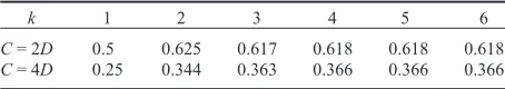
In Broom et al. (2000) the case whereV_k– V_{k +1}=

=D"kwas considered for bothC= 2DandC= 4D,

each forn = 1, …, 6. We now revisit this example

and compare the two models. Note that hereb_k is

constant overk, and thatb=D/C; we can thus use

the above working to find the candidate ESS for each case. The ESO value of the probability of play-ing Hawk in each round is shown in Table 1. The

ESO withkrounds to go is not affected by the total

number of rounds, and so the best play for any

num-ber of rounds n less than 6 is given by columns

headed 1, …,nin Table 1.

This yields the expected number of violent Hawk versus Hawk contests as shown in Table 2. The cor-responding values for the fixes strategy case are shown by way of comparison. It is clear that there is far more conflict in the variable strategy case than the fixed strategy case, for identical tournament

TABLE1

C= 2D,C= 4Dthe probability of playing Hawk in roundk

k 1 2 3 4 5 6

C= 2D 0.5 0.625 0.617 0.618 0.618 0.618

C= 4D 0.25 0.344 0.363 0.366 0.366 0.366

TABLE2

The proportion of Hawk v Hawk contests over the whole con-flict;C= 2DandC= 4D

n 1 2 3 4 5 6 ∞

C= 2D,Fixed 0.25 0.282 0.280 0.270 0.262 0.257 0.252

C= 2D,Variable 0.25 0.344 0.365 0.374 0.378 0.380 0.382

C= 4D,Fixed 0.063 0.078 0.079 0.072 0.064 0.056 0.041

[image:8.595.305.532.488.528.2]

structures. Thus extra choice has greatly reduced the payoffs to individuals. Of course, in a population of fixed option players, an individual who plays a suit-ably varied strategy would invade; evolution can re-duce the fitness of the population.

b) Degenerate cases

b(i) If∆= 0 then a player has a probability of

win-ning of ½ whichever opponent it is playing i.e. the

rewardV_iattained is independent of the play so that

the game reduces to a series of pairwise games with payoff matrix.

− −

− −

 

 c_c11 _cc12_ 21 22

.

b(ii) If all the costs are zero then C₁+ C₂ = 0 and

y_{k+ 1 =}y_k/2+ a_k. All thea_k’s are positive (since∆> 0) so thatp_k= 1∀k.

c) Symmetric costs with

c₁₂=c₂₁= 0,c₁₁=c₂₂=C> 0.

Here players incur a cost if losing to an opponent playing the same strategy, but not if they lose to an opponent playing the other strategy, as is perhaps reasonable since the latter can be easily and quickly resolved.

c₁₁=c₂₂=C⇒C₁=C₂=C/2 > 0

zk+1 =zk +bk + pk −pk −

2 ∆ (1 )

1 2

1

11 22 1 2 ∆c p c p

C C

k + − k

+ =

( )

zk _{b p p}

k k k

2 1

1 2

+ +∆ ( − )− ∆.

We have assumed thatV_k– V_{k+ 1}is constant over all

values ofk. Defineαby letting Cα =V₀–V₁, then

b_k= 1/4 +∆αso that

zk+1 =zk + − + + pk −pk 2

1 2

1

4 1

∆α ∆ ∆ ( ).

For a very large number of roundsp_kwill tend to a

constant value which is given by the equation

p p= + − + + p −p 2

1 2

1

4 1

∆α ∆ ∆ ( ),

ifαis sufficiently small (otherwisep= 1 is the

equi-librium value). In case of the game when∆= 1/2 i.e.

p p= −1 p + ⇒ =p 2

1 2

2 _{α α}

for α < 1, otherwise p = 1. It follows that even

though the rewards are increasing in value andO₁

-players have a better chance of progressing further

in the competition thanO₂-players for small α the

overwhelming number of players in the equilibrium

case play O₂ despite the symmetric appearance of

the costs. The reason for this is that for large values

ofCthe priority of the players is to leave the game

without incurring a cost, and for∆= ½ the only way

of achieving this is playingO₂against aO₁-player.

We now examine when such a candidate ESS

from case (i) is actually an ESS, considering the

sim-plest non-trivial case, namely the game with two rounds.

2.4. Unstable equilibria

Consider the knockout game where there are two rounds and two options. We assume that there is a

candidate ESS, labelled p, with (internal) ESOsp₁in

round 1 andp₂in round 2. Suppose that a group of

size∈playing q = (q₁,q₂) tries to invade a popula-tion all of whose members play p. We evaluate the expected payoff to a p-player minus the expected payoff to a q-player and thus show when q can in-vade. In particular we find conditions for when no such q can invade i.e. when p is an ESS.

The mathematical arguments involved to show this are in Appendix B. It is shown when q can in-vade p, and that p is an ESS, if and only if

∆ ∆2 1 ∆

2

0 1 21

(V −V )+ + c



 

  − 

 

1

2 12 2

1 2

1 2 −

 

 

  

< + ∆ c (C C ).

Note thatV₂ does not appear in this inequality, so

that the value ofV₂does not affect whether our

can-didate ESS is in fact an ESS (of courseV₂affects the

value ofp₂; in particularp₂is not internal unlessV₂ lies within a certain range). For Example 1, we have

C₁+ C₂= 2 so that the right-hand side of the

There is a parallel with extensive two-person games here, although not an exact one. Van Damme (1991) showed that an LSS is not always an ESS (see Cressman and Schlag, 1998 for a discussion on when backwards induction is a useful method to solve extensive form games). He constructed an ex-ample, similar to the knockout idea, where players either played a second stage or stopped after the first stage, depending upon play at the first stage. In this game either both players play a second stage or nei-ther do, the mutant invading by playing so that mu-tant v mumu-tant contests were likely to play the second stage, and playing cooperatively in the second stage. In our game the situation is different; a player can only increase its chances of progressing at the cost of its opponent. The mutants either play aggres-sively at first, so that more mutants reach the next stage, and then play passively or the converse, as in Section 2.5. Thus the mutant can indirectly make it marginally more (or less) likely that the next oppo-nent it faces is also a mutant, and behave accord-ingly. This is a less effective mechanism than that available in the two-person extensive games, so it is reasonable to think that the knockout models are more likely to have ESSs.

2.5. Petal dynamics in knockout games

2.5.1. The replicator dynamic

Suppose that for a particular evolutionary game, the

strategies which a player may play are S₁, …, S_n

(these may be pure strategies, or ‘allowable’ mix-tures as in the example we consider). Let the propor-tion of players ofS_iat a particular time bep_i(i= 1,

…,n), so that the average population strategy is the

vector p = (p_i), with the expected payoff (in terms of

Darwinian fitness) of anS_i-player in such a mixture

being f_i(p) and the overall expected payoff in the

population beingF p( )=

∑

p f pi i( ). Then the stan-dard replicator dynamic (continuous) is defined by the differential equation

dp

dt p f p F p i

i i

= [ ( )− ( )].

Thus the proportion of players which play the better strategies increases with time (what determines a good strategy depends upon the composition of the

population). A point inn-dimensional space,

repre-sented by the vector p, is locally stable if it is an ESS [this is not necessarily true for the discrete dynamic (Zeeman, 1980)]. The replicator equation has been applied in very many situations (see Hofbauer and Sigmund, 1988).

We shall revisit Example 1. The parameters are as follows:

V₀= 7.5,V₁= 6.5,V₂= 0,

c₁₁= 25,c₁₂= 0,c₂₁= 11,c₂₂= 1,∆= 0.5. We have previously shown that (0.5, 0.5) is a Nash equilibrium but not an ESS. In order to study the possible invasion of a population playing v by some

alternative playing u we need to evaluate W₂(u, v)

the expected future payoff to a u-player who wins in round 2. We have u = (u₁, u₂) and v = (v₁, v₂) and

W₂(u, v) depends only onu₁andv₁, and is given by

W₂(u, v) = (u₁, 1 –u₁) M₁(v₁, 1 –v₁)T_{. (3)}

To illustrate we shall consider the set of nine possi-ble strategiesr_ij, (i,j= 1, 2, 3) wherer_ijplaysx_iin round 1 andx_jin round 2, wherex₁= 0.1,x₂= 0.5 and

x₃= 0.9. Thusr₂₂is the Nash equilibrium. Under this

regime, we have from equation (3) that

W₂(r_ij,r_kl) = (x_i, 1 –x_i) M₁(x_k, 1 –x_k)T_,

which we denote byW₂(i, k), since there is no

de-pendence onjorl, and the matrix W₂ofW₂(i,k)

ele-ments fori,j= 1, 2, 3 is given in this case by

25

137 25 87

145 25 95

153 25 103

W2 =

− − − 

   



   

.

Now consider round 2. For strategies which playi

andkin round 1 we have payoff matrix M₂(i,k) in

round 2 given by

M2 2 2

2

25 2

11 1 2

( , ) ( ( , ) ) / ( , )

( ( , ) ) /

i k W i k W i k

W i k

= −

− −

 

 

 ,

which we write as

M₂(i,k) =W₂(i,k) A + B (4)

ex-pected payoff for r_ij in a population of r_kl players, which we denote byM₂(r_ij,r_kl) is given by

M₂(r_ij,r_kl) = (x_j, 1 –x_j) M₂(i,k)(x_l, 1 –x_l).

Substituting from equation (4) we have

M₂(r_ij,r_kl) =A₂(j,l)W₂(i,k) +B₂(j,l)

whereA₂(j,l) = (x_j, 1 –x_j)A(x_l, 1 –x_l) andB₂(j,l) = = (x_j, 1 –x_j)B(x_l, 1 –x_l),A₂(j,l) andB₂(j,l) being the probability of winning in round 2 and the expected

costs, for aj-player against an opponent playinglin

that round. The matrices A₂and B₂, are given by

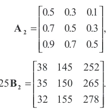
A2 =



   



   

0 5 0 3 01 0 7 0 5 0 3 0 9 0 7 0 5

. . .

. . .

. . .

,

25

38 145 252 35 150 265 32 155 278 B2 =



   



   

.

The relative values ofM₂(r_ij,r_kl) =

(x_l, 1 –x_j)M₂(i,k)(x_l, 1 –x_l) are given in Table 3.

By inspecting the entries in Table 3, we can iden-tify those strategies which can invade any popula-tion. A strategy u can invade a population playing v if, in column-v (that is the column corresponding to v) the entry in row-u exceeds that in row-v (i.e. E[u, v] >E[v, v], or if these are equal then if, in col-umn-u (that is the column corresponding to u) the

entry in row-u exceeds that in row-v (i.e.E[u, u] >

E[v, u]). For example only (1, 3) and (3, 1) can

in-vade (2, 2); that is only (0.1, 0.9) and (0.9, 0.1) can invade the Nash equilibrium (0.5, 0.5). Table 4

con-tains the complete set of information regarding which strategies can invade which monomorphic populations; if the entry in row (i,j) and column (k,

l) is + then the former can invade a population of the

latter.

We observe that there are sequences of strategies, labelled {s₁,s₂, …,s_u} say, such thatsu invades s1

ands_iinvadessi+ 1fori= 1, …,u– 1. In particular

{(0.5, 0.5), (0.5, 0.1), (0.9, 0.1)}

is such a set and we investigate the dynamics of this particular set in more detail below.

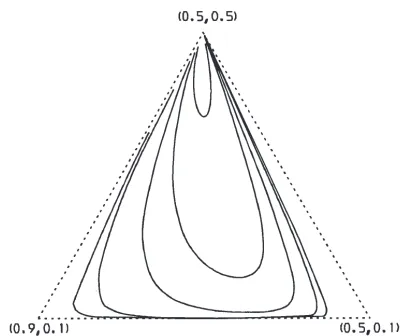
2.5.2. Phase portraits for three strategies

For games with three strategies, the proportion in the population of each of the strategies can be repre-sented upon an equilateral triangle of unit height. Since the triangle is equilateral the sum of the per-pendicular distances from each edge is equal to the height of the triangle, and thus is 1. Each strategy, therefore, can be represented by one of the vertices with the proportion of this strategy being the perpen-dicular distance from the opposite edge. For exam-ple, if the population all play strategy 1, then the cor-responding point in the triangle is the vertex representing that strategy; if the population plays strategies 2 and 3 with equal probability, the corre-sponding point is midway along the edge between the vertices associated with strategies 2 and 3.

If we make a small disturbance away from the equilibrium (adding a small proportion of players of the other two strategies), the behaviour follows the

TABLE3

Relative payoff of strategy (i, j) (row-label), in a population of (l, k)-players (column-label)

(1, 1) (2, 1) (3, 1) (1, 2) (2, 2) (3, 2) (1, 3) (2, 3) (3, 3) (1, 1) 305 –255 –815 –1039 –1375 –1711 –2383 –2495 –2607 (2, 1) 345 –255 –855 –1015 –1375 –1735 –2375 –2495 –2615 (3, 1) 385 –255 –895 –991 –1375 –1759 –2367 –2495 –2623 (1, 2) 609 –175 –959 –815 –1375 –1935 –2239 –2575 –2911 (2, 2) 665 –175 –1015 –775 –1375 –1975 –2215 –2575 –2935 (3, 2) 721 –175 –1071 –735 –1375 –2015 –2191 –2575 –2959 (1, 3) 913 –95 –1103 –591 –1375 –2159 –2095 –2655 –3215 (2, 3) 985 –95 –1175 –535 –1375 –2215 –2055 –2655 –3255 (3, 3) 1057 –95 –1247 –479 –1375 –2271 –2015 –2655 –3295

TABLE4

Specification of invasions possible

(1, 1) (2, 1) (3, 1) (1, 2) (2, 2) (3, 2) (1, 3) (2, 3) (3, 3)

(1, 1) 0 – + – – + – + +

(2, 1) + 0 + – – + – + +

(3, 1) + – 0 – + + – + +

(1, 2) + + – 0 – + – + +

(2, 2) + + – + 0 + – + +

(3, 2) + + – + – 0 – + +

(1, 3) + + – + + – 0 – +

(2, 3) + + – + – – + 0 +

(3, 3) + + – + – – + – 0

[image:11.595.125.235.272.386.2] [image:11.595.63.291.470.590.2]

pattern in Figure 1, with its path in the shape of a petal (at least for small disturbances). The popula-tion can move very far from the equilibrium if most of the introduced group plays (0.9, 0.1) no matter how small the disturbance (if the group is entirely (0.9, 0.1) then the population follows the edge of the triangle until the whole population plays (0.9, 0.1)). The size of the ‘petal’ decreases the larger the (0.5, 0.1) component in the added group, however as long as this component is non-zero the population always returns to the equilibrium. Hence even for a small disturbance, the population can spend a long time away from the equilibrium (which is unstable), but the dynamic will move the population back to the equilibrium eventually. This ‘petal’ phenomenon was discussed in Hofbauer (1993). There is another parallel with extensive two-person games here. Cressman (1997) proved that under certain condi-tions solucondi-tions obtained using backwards induction,

as in Selten (1983), werelocally asymptotically

sta-ble, so that the evolutionary dynamic eventually

re-turned the population to such a solution, even if it was not an ESS; this is precisely what happens in our case.

2.6. The three-option case

We now briefly examine the knockout game where there are three options to show how the ideas already discussed can be adapted to consider more than two

options. The payoff matrix for players in a particular round conditional upon future rounds is shown and an outline of how to find ESOs is given. In general there may be up to three (or indeed no) ESOs of a round for the three-option case, conditional on the play in lower numbered rounds. We then describe the conditions for which every ESO includes all three options (and is thus unique).

Finding the ESOs

The rewards, costs and the probability of victory against other strategies are as described earlier in

this section. LetW_kagain be the expected payoff for

winning in round k. For 2-player matrix games, sub-tracting a constant from every element in a column of a matrix does not affect the ESSs of that matrix (Zeeman, 1980). Thus subtracting a constant from

the matrix of payoffs for roundkdoes not affect the

ESOs of that round. We shall subtract the leading di-agonal element from each column. Then the three-player game has the following payoff matrix for

roundk:

( )

( ) (( ) )

M

c c

W V c

c c

W V c

k

k k k k

=

− +

− +

− −

− +

0 1 2 22 12 1 2

12 12

33 13 31 13

/ /

∆ ∆

( )

( ) (( ) )

1 2

0 1 2

1 2

11 21 12 21

33 23 23 23

/ /

/

c c

W V c

c c

W V c

k k k k

− −

− +

− +

− +

∆ ∆

( )

(Wc Vc c ) (( ) )

c c

W V c

k k k k

11 31 31 31

22 32 23 32

1 2

0

− +

− +

− −

− +



    

∆ ∆

/ 

  



         .

Three strategy games and their ESSs are discussed in Vickers and Cannings (1988), and their results can be readily used to find the ESOs of the above matrix.

An internal ESO is one in which the probability of playing a given pure option is greater than zero for all of the options. We can find a recurrence rela-tion between ESOs in successive rounds in a similar

manner to Section 2.3. Definingr_k=W_k–V_kandD_k=

V_k–V_{k+ 1}then equation (1) yields the following

re-currence relation forr_k.

2r_{k+ 1}=r_k+ 2D_k– 2X_k

Thus, sincer₁=V₀–V₁, we can find the value ofrk

for every round and it is shown in Appendix C that there is an internal Nash equilibrium (p_1k, p_2k, p_3k) where

p y

y y y

ik ik

k k k

=

+ +

1 2 3

FIG. 1. Trajectories of the composition of the population for a 2-round knockout game with three strategies. The marked trajec-tories represent invasions into a population of (0.5, 0.5)-players by a small group containing (0.9, players and (0.5, 0.1)-players. As the proportion of (0.9, 0.1)-players increases the

[image:12.595.77.277.82.250.2]

and

y1k =∆ ∆23 rk +C r C11 k + 12

2

y2k =∆ ∆31 rk2 +C r C21 k + 22

y3k =∆ ∆12 rk2 +C r C31 k + 32

ify_ik> 0∀i, where all the parametersC_ijand∆_ij are defined in Appendix C.

The Nash equilibrium is also an ESO if the matrix satisfies the negative-definiteness condition of Vickers and Cannings (1988). This depends upon the costs only, and so if satisfied for one round it is satisfied for all and vice versa. Thus it is possible to generate the unique Nash equilibrium for the whole game.

3. Discussion

The knockout model provides an example of a situa-tion where all conflicts in a populasitua-tion are pairwise, but are organised into a structure and thus not inde-pendent. This is not necessarily a realistic model of the way natural populations behave, but rather gives an insight into natural conflicts and how (and in what way) behaviour may be much more complex than that predicted by classical 2-player game the-ory. The dependence between games leads to behav-iour which is qualitatively different to that from con-tests where the pairwise concon-tests are independent.

It was shown in Broom et al. (2000) that there may be more or less aggression in a population play-ing a contest with a knockout format than in inde-pendent pairwise games, providing that there is no possibility of adjusting the strategy from round to round, depending upon the number of players and the rewards and costs involved. In Section 2.3 we see that when there is free choice of behaviour from round to round, the level of aggression increases the more rounds there are, and is more than for inde-pendent contests. Thus this freedom is damaging to the individuals, but will nonetheless evolve into the population.

In Section 2.3 it is shown that for a population

or-ganised into an nround knockout tournament with

two available options, in the variable option case

there may be as many as 2n_{ESSs, but there is a}

sim-ple commonly satisfied condition which if satisfied guarantees at most one ESS. It is shown in Section

2.4 that there might be no ESS at all (in 2-player game theory there is always an ESS when there are two strategies). It appears that any Nash equilibrium is less likely to be an ESS than for classical theory,

since even the existence of a sequence ofESOs is not

sufficient to guarantee an ESS. Thus there are extra conditions to be met for a strategy to be an ESS than in 2-player game theory. In particular a completely internal equilibrium is especially susceptible to in-vasion; the more pure options involved in the ESOs which make up the Nash equilibrium strategy the more susceptible it is (similarly, the more rounds, the more susceptible it is). Thus in real populations the number of observed options which occur in real-ity might be lower if there is a structure to the games that are played. However, it should be noted that there is a reverse tendency as well, since different pure options may be involved in the ESO for differ-ent rounds, thus increasing the overall number of pure options used in total.

As we have seen, the game can be very complex if players are able to change their strategies from round to round. For two options, strategies are vec-tors not just single numbers (for more than two op-tions they are matrices rather than vectors). A recur-sive dynamic programming method was found which specifies all the candidate ESSs of a game. Showing when a candidate ESS is actually an ESS is a harder problem. In Section 2.4 we do this for the 2 round case. The method used can be generalised to more rounds, but calculations quickly become complicated. Section 2.5 shows that the dynamics of these games is also more complex than those for 2-player games. Indeed the example given is the simplest possible non-trivial knockout game

(2-round, 2-option∆= ½) and it is to be expected that

even more complicated behaviour will result from a more complex game. There is an interesting corre-spondence between the knockout model and the ex-tensive two-person game of Selten (1983), which deserves to be explored further.

Acknowledgements

APPENDIX

A) A recurrence relation foryk

The following argument finds a recurrence relation

fory_k. In general for a population playing the mixed

strategy (p₁, …,p_n) each placer has a probability of ½ of being eliminated in any round, and the

ex-pected cost for a player in roundkis

Xk =p ck2 11 + −pk 2 c22 +

2 (1 ) 3

pk(1 pk) 1 c c .

2

1 2

21 12

−  + 

 



 + − 

 

  



 ∆ ∆ _

It follows that

Wk =Vk−1 +Vk−2 + + V_k1₋₁ + V_k−0₁ −

2 4 ... 2 2

− _{− −} = −

= −

∑

Xi _{k i} v Yk k i

k ₁

2 1

1 1

where

Yk X_k k _i i

k

= _{− −}

= −

∑

₂ 1 1 1

Y_k is thus the expected future cost incurred by a

player which wins in roundkand

Yk X_k k_i Y Y X i

k

k k k

= _{− −} ⇒ = +

= −

+

∑

₂ 1 ₂

1 1

1 .

It is now possible to findy_{k+ 1}in terms ofyk.

Wk+1 =vk+1 −Yk+1 =vk +Vk −Yk −

2 2 2

−Xk(2v Vk = k +vk−1)

⇒Wk+1 =Wk +Vk −Xk

2 2

⇒2(Wk+1 −Vk+1) (= W Vk − k)+

2(V Vk − k+1)−2Xk

⇒ 2C1 +2∆(Wk+1 −Vk+1)=

=∆(W Vk − k)+C1 +2∆(V Vk − k+1)+C1 −2∆Xk

⇒ yk₊1 =yk +ak − Xk

2 ∆

(a_kis as defined in Section 2.3).

We now rearrange the expressionX_kto get it into

a more manageable form.

Xk =p ck2 11 + −pk 2 c22 +

2 (1 ) 2

pk(1 pk) 1 c c

2

1 2

21 12

−  + 

 



 + − 

 

  



 ∆ ∆ _

=p Ck2( 1 +C2)+

pk−C −C +c −c c



 

  + 1 2 11 22 22

2 2 2

⇒Xk = −(C1 +C p2) (k 1−pk)+

1

2[c p11 k +c22(1−pk)].

B) Conditions for an ESS for the 2 round 2-player game

Notation

We define and then evaluate a series of terms which help us to find whether p is an ESS.

h_i: the proportion of O1-players in round i,

i = 1, 2.

g_i(r): the probability of an r-player playing in

roundiwinning,i= 1, 2, r = p or q.

vi(r): the expected contribution to the payoff of an

r-player of a loss in roundi, i= 1, 2, r = p or q.

E(r): the expected total payoff of an r-player in

the game, r = p or q.

Also defineu₁= (p₁–q₁)[1 – 2∆(p₂–q₂)] andu₂= (p₂–q₂).

The above expressions can be used to find the

payoff functions E(p) and E(q), and in particular

their difference.

E(p) =v₂(p) +v₁(p) +g₂(p)g₁(p)V₀,

E(q) =v₂(q) +v₁(q) +g₂(q)g₁(q)V₀

⇒E(p) –E(q) =

[v₂(p) –v₂(q)] + [v₁(p) –v₁(q)] +

ESS conditions

Thus we nee to evaluate all the terms given in (5). These equations are labelled (6–18); some lower numbered equations are required to solve those which come later. An indication of which (if any) are required is given after each equation.

h2 =p2(1− +ε) q2ε=p2 −εu2 (6)

g2 1 p2 h2 p2 q2

2

1 2

( )p = +∆( − )= +∆ε( − )

= +1

2 ∆εu2 (7)

using (6).

g2 1 q2 h2 p2 q2

2

1

2 1

( )q = +∆( − )= −∆( −ε)( − )

= −1 −

2 ∆(1 ε)u2 (8)

using (6).

h1 =2 1( −ε)p g1 2( )p +2εq g1 2( )q

=p1 −ε(p1 −q1)+2 1( −ε ε) ∆(p2 −q2)(p1 −q1)

=p1 −εu1 −2ε ∆2 u p2( 1 −q1) (9)

using (7) and (8).

g1 1 p1 h1

2

( )p = +∆( − )=

= +1 + −

2 1 2

2 2

2 1 1

∆εu ε ∆ u p( q ) (10)

using (9).

g1 1 q1 h1

2

( )q = +∆( − )=

= −1 − + + −

2 1 1 1 2

2 2

2 1 1

∆(p q ) ∆εu ε ∆ u p( q ) (11)

using (9).

v2 1 V2 c p h11 2 2

2

( )p = ( − ) +

1

2− 2 12 2 1 2

 

 



 − − +

∆ (V c p) ( h )

1

2+ 2 21 1 2 2

 

 



 − − +

∆ (V c )( p h)

1

2(V2 −c22)(1−p2)(1−h2) (12)

using (6).

v2 1 V2 c q h11 2 2

2

( )q = ( − ) +

1

2− 2 12 2 1 2

 

 



 − − +

∆ (V c q) ( h )

1

2+ 2 21 1 2 2

 

 



 − − +

∆ (V c )( q h)

1

2(V2 −c22)(1−q2)(1−h2) (13)

using (6).

v1( )p =g2( )p 1₂(V1 −c p h11) 1 1 + 

1

2− 1 12 1 1 1

 

 



 − − +

∆ (V c p) ( h )

1

2+ 1 21 1 1 1

 

 



 − − +

∆ (V c )( p h)

1

2(V1 −c22)(1−p1)(1−h1)

 

 (14)

using (7) and (9).

v1 g2 1 V1 c q h11 1 1

2

( )q = (q)_ ( − ) +



1

2− 1 12 1 1 1

 

 



 − − +

∆ (V c q) ( h )

1

2+ 1 21 1 1 1

 

 



 − − +

∆ (V c )( q h)

1

2(V1 −c22)(1−q1)(1−h1)

 

 (15)