A black-box dynamic equivalent model for microgrids using measurement data

A Black-Box Dynamic Equivalent Model for Microgrids Using

Measurement Data

Panagiotis N. Papadopoulos1_{, Theofilos A. Papadopoulos}1_{, Paul Crolla}2_{, Andrew J.}

Roscoe2_{, Grigoris K. Papagiannis}1_{, Graeme M. Burt}2

1_{Power Systems Laboratory, Dept. of Electrical & Computer Engineering,}

Aristotle University of Thessaloniki, P.O. Box 486, GR-54124 Thessaloniki, GREECE Tel: +302310996388, Fax: +302310996302, e-mail: [email protected]

2_{Institute for Energy and Environment, Department of Electronic and Electrical}

Engineering, University of Strathclyde

Tel: +4401415482951, Fax: +4401415485872 e-mail: [email protected]

Abstract

A dynamic equivalent black-box model, based on Prony analysis is presented in this paper. The proposed model is suitable for dynamic studies of microgrids, considering changes in the active and reactive power, bus voltages, currents and frequency. The developed model is evaluated using simulation results obtained from a medium voltage microgrid and test measurements recorded in a low voltage microgrid laboratory test facility. Results from the proposed model are in good agreement with the corresponding responses obtained from both simulations and laboratory tests. The examined microgrid configurations include rotating machines and inverter interfaced units implementing different control strategies, thus verifying the robustness of the proposed model.

Keywords

1. Introduction

In recent years the number of Distributed Generation (DG) units has increased rapidly, influencing the operation and the performance of power systems and especially distribution networks. To facilitate the analysis of such distribution grids the concept of microgrid (MG) has been introduced, containing different types of DG units, either renewable or conventional with or without energy storage devices [1], [2]. Due to the stochastic nature of renewable sources and the effect of the complex control strategies of the DG units, frequent changes in the network topology and the operating conditions of the DG units occur, influencing significantly the dynamic behaviour of the system [3]. Therefore the development of accurate and adaptive dynamic simulation models of MGs is essential, in order to enhance the DG utilization and investigate more efficient ways of operation [4].

There are several cases in the literature using detailed models to investigate the dynamic behaviour of MGs [5]-[7]. This approach however demands significant computational power and large simulation times for extended MG systems with large number of DG units and complex control schemes. There are also several other drawbacks, such as the lack of detailed information about the design and control parameters of DG units as well as the difficulties to incorporate efficiently the constant change of the generation mix and the network topology.

To overcome the computational effort difficulties, reduced order models for MGs have been proposed, based on the same techniques previously used for the simulation of large-scale power systems. In [8] reduced order models are presented, based on eigenanalysis and Prony analysis and in [9] the Hankel-norm approximation is adopted. Similarly, a coherency identification based equivalent model is proposed in [10] whereas in [11] the same method has been implemented in the dynamic reduction program DYNRED. Dynamic equivalencing techniques are also widely used to implement reduced order simulation models, specifically for the case of wind farms [12], [13]. However, the identification of parameters in reduced order models also requires network information, thus the previous restrictions and drawbacks apply to this category as well.

and the network topology, and improve the numerical performance of the simulation. In both models the parameters are extracted mainly from measurements, using system identification techniques. However, in the black-box approach no prior knowledge of the model structure is required, while in the grey-box some initial information is necessary. Furthermore, modelling restrictions due to the network complexity, generation mix and control strategies are overridden by the black-box approach, ensuring the flexibility and generalized form of the developed models. The black-box parameters are derived using system identification techniques such as sub-space methods [17], [18] and Prony analysis [19], [20]. In most cases simulation results are used for the model parameter identification and validation, whereas in some cases field measurements from conventional, extended transmission networks [19].

In this paper a black-box dynamic model, suitable for the simulation and analysis of MG systems is presented. It is based on Prony analysis and nonlinear least square optimization, as in [20]. The model represents the dynamic performance at a reference point of the MG, when the MG is subjected to small disturbances and thus can be used for small signal stability analysis. The reference point can be the Point of Common Coupling (PCC) or a DG unit point of coupling within the MG. The model outputs are the dynamic responses of the active and reactive power, the bus voltage, the current and the frequency in a modular structure with decoupled system variables. Measurement data are used to extract the model parameters, which can be updated online, providing an accurate representation of the changing system structure. The model can be combined with power system analysis software packages and can be implemented as a portable network feeder element, representing the MG system [14], [18]. The proposed model is used in several MG topologies including both rotating and inverter interfaced DG units with different control strategies. The influence of the above parameters on the calculated Prony terms, the model response and the dynamic behaviour of the MG system are investigated systematically. The model is also validated using measurement test data recorded in a laboratory scale MG system at the University of Strathclyde, UK [22].

A. Black-Box modelling fundamentals

Traditionally, Prony analysis has been used in large power transmission system studies as in [17] and [19], where slow transients up to a few decades of seconds have been simulated. The proposed model focuses on the representation of the dynamic behaviour of microgrids, where transients involved are generally faster and with larger damping, due to the small inertias of the rotating DG units and the resistive behaviour of the microgrids [5], [6], [14]-[16].

The model is based on Prony analysis and nonlinear least square optimization in order to identify the system eigenvalues from recorded dynamic responses at a reference point of the MG and represent the MG dynamic behaviour. The model outputs can be the active (P) and reactive power (Q), both of which can be incorporated in power system analysis software as a feeder element suitable for small signal stability analysis, as well as the bus voltage (V), system frequency (f) and current (I), which can be used for voltage/frequency stability analysis and dynamic studies.

Prony analysis provides an efficient way to fit a dynamic response with a sum of damped sinusoids [19], [20], [23]. However, for each individual disturbance in a MG configuration (different disturbance amplitude or pre-disturbance steady state condition of the MG) a new set of Prony terms must be extracted, resulting in a huge amount of data and considerable computational burden. The proposed model, in contrary to [20], overcomes this inherent restriction by implementing additional correction factors, limiting the required data for the estimation of the model parameters.

The proposed model is suitable for the analysis of small signal dynamics of MGs, when subjected to small internal disturbances, e.g. changes in the load power and the operational conditions of DG units. Therefore, the investigated dynamic disturbances are considered large enough to influence the system dynamics and small enough to ignore nonlinearities in the system [24].

B. Model formulation

interaction of the other system variables caused by the actual system control loops.

ˆ _{  } ˆ _{ }

tr 0

Y ΔY U Y U Y (1)

where





ˆ _{ˆ ˆ ˆ ˆ ˆ} T ˆ ˆ ˆ T

y y y y y P Q V I f

 _{  }

Y (2a)



 



T T

0 0 0 0 0

y y y y y P Q V I f

 

0

Y (2b)









diag y y y y y diag P Q V I f

 

ΔY (2c)





ˆ _{ˆ ˆ ˆ ˆ ˆ} ˆ ˆ ˆ

tr tr tr tr tr tr tr tr tr tr

diag y _ y _ y _ y _ y _ diag P Q V I f 

  _{ }

tr

Y (2d)

         

U (2e)

Function u(t) _{is the unit step,} Yˆ is the output vector, Y0 represents the MG

pre-disturbance steady state condition and ΔY _{is the input vector and includes the step} changes Δym. All vectors are of order M, which is the total number of the system

variables. Function yˆ_{tr m}

 

system variable and is fitted by a sum of Nm Prony terms as given in (3).

1 1

1

( ) cos( ),

2

m m

mn mn mn

N N

j t t

tr m mn mn mn mn

n n

y _ t A e e A e  t 

 







Parametersmn, mn and mnmn jmn are the amplitude, phase and model

eigenvalue, respectively and _mn, _mn are the corresponding angular frequency and the

damping coefficient [24]. Each Prony term is the result of the sum of complex conjugates and represents a damping oscillation. The proposed model has a generalized form, since by selecting properly the order Nm of the corresponding model subsystem, it

can include all types of generation units, control schemes and load types. A change in the topology of the MG is represented by introducing or subtracting the corresponding Prony terms in (3).

C. Parameter identification

software packages.

First, the model initialization is based on a random system disturbance and its preceding steady-state condition. This set of events defines a base scenario for the model. The dynamic response of the MG at the reference point is recorded for the base scenario, as well as for two additional disturbances; one of different amplitude and one of different pre-disturbance steady state condition than the base scenario.

[Fig. 1]

Next, the model parameters Amn, ωmn, σmn, and φmn of (3) are extracted for each of the

three datasets, using Prony analysis to get an initial estimation [17], [19], [23], [24], while the initial operating condition y0m is acquired directly from the corresponding

measurement data. The appropriate number of Prony terms for each system variable, and thus the order of each subsystem can be identified using the subsystem identification method N4SID [25], available in MATLAB [26]. In certain cases, especially for non-oscillating responses, the proposed system order can be further reduced by trial and error methods. In all cases presented in this paper, two Prony terms proved enough to lead to satisfactory performance. Since the accuracy of Prony analysis is usually not very high, the nonlinear least square optimization technique is also applied to improve the initial parameter estimation as in [20]. The curve fitting tool of MATLAB [26] is adopted for this purpose, using the trust-region algorithm. Similar results are also obtained, using the Levenberg-Marquardt and Gauss-Newton methods available also in MATLAB. For the nonlinear least square optimization procedure an initial value as well as a lower and upper boundary for each of the estimated parameters must be specified. The initial values are derived from Prony analysis, while proposed empirical guidelines are used to initialize and adjust the boundary values, in order to reach the predefined error criteria. The estimation procedure target is to minimize the root mean square error (RMSE) and also maximize the coefficient of determination (R2) defined in (4) and (5), respectively [26]. According to the results from numerous

number of iterations and thus the required execution time of the proposed method.

 



 

 



1 1

ˆ

min _m min Km _{m m}

k m

RMSE y y k y k

K 

 

 

   

 

 





(4)

 

 

_{ }

2

max_  _ max 1_  _

 

m m

m

SSE y R y

SST y (5a)

where

 



 

 



1

ˆ







m m m

k

SSE y y k y k (5b)

 



 



1







m m m

k

SST y y k y (5c)

where y_{m and} yˆ_mare the original and estimated values of the system variables,

respectively, y_m is the mean value and K_m the corresponding number of samples. The adopted empirical guidelines are summarized below:

 The initial values for the nonlinear least square optimization are provided by Prony analysis. The boundaries of the Prony terms are set according to the corresponding initial value as ± 10% for the ωmn term, ± 100% for the Amn term, ± 50% for the σmn

term and -2π up to 2π for the φmn term.

 Fourier analysis can be additionally applied for the initial estimation of the ωmn

parameter in case Prony analysis results are not accurate.

 If the RMSE and R2 targets are not met, the initial parameter estimation value and the corresponding boundaries are increased until the error targets are met. If the errors become worse the initial values are decreased.

parameters immediately.

D. Model correction factors

Next, the model correction factors are calculated. The eigenvalues λmn and phase φmn

of all system variables can be considered constant as calculated from the base scenario, since the system is assumed linear. However, parameter Amn strongly depends on the

disturbance amplitude and the pre-disturbance steady state condition of the MG as depicted in Fig. 2, showing in general a linear behaviour.

[Fig. 2]

Therefore, the behaviour of parameter Amn against the disturbance amplitude and the

pre-disturbance steady-state condition of each Prony term is approximated by the linear correction factors CF1mn and CF2mn, as shown in (6)-(8).

ˆ

mn mn mn base mn

A CF1 CF2 A _ (6)

1

mn mn mn

CF1 a1 x b1 (7)

2 2mn 2mn 2mn

CF a x b (8)

where Abase-mn is the corresponding parameter of the base scenario. CF1mn approximates

linearly the variation of Amn against the disturbance amplitude, while similarly the

pre-disturbance steady state condition variation is represented by CF2mn. Variable x1

indicates the percentage change of the disturbance amplitude from the nominal operating condition, as an absolute value. On the other hand, variable x2 indicates the

percent change from the pre-disturbance operating condition of the base scenario. Therefore x2 is always zero for the base scenario while x1 can take any value depending

on the available measurement set. Since correction factors are linear functions, two points are required in order to determine their values. For each correction factor one point is acquired from the base scenario, while the other from the additional dataset, thus the resulting total number of the minimum required measurement datasets is three. Parameters a1mn and a2mn express the slope of CF1mn and CF2mncurves, therefore their

sign and magnitude show the monotony and sensitivity of the corresponding Amn

condition changes.

Finally, taking into account the correction factors for each Prony term the proposed black-box model described by (1) is rewritten in (9).

1 1 1

2 2 2

3 3 3

4 4 4

5 5 5

0 0 0 0 0 0 0 0 ( )

0 0 0 0 0 0 0 0 ( )

0 0 0 0 0 0 0 0 ( )

0 0 0 0 0 0 0 0 ( )

0 0 0 0 0 0 0 0 ( )

tr

tr

tr

tr

tr

y y y

P u t

y y y

Q u t

y y y

V u t

y y y

I u t

y y y

f u t

                                                                                            1 2 3 4 5 0 0 0 0 0 y y y y y                            _{  } , (9a) where 1 ˆ

( )  cos(  ),









N

t

tr m mn mn mn

n

y t A e t (9b)

and Aˆ_mn are calculated using (6)-(8).

E. Model characteristics

The most significant advantages of the proposed model are summarized below:

 The black-box approach eliminates the need for information considering the topology and the operating condition of the MG, relying solely on recorded dynamic responses.

 Only the dominating eigenvalues affecting the dynamic response of the system are identified.

 The parameter identification algorithm is computationally efficient, requiring approximately 30 s for each loop of Fig. 1 in a typical personal computer, after the measurement data sets are available. Therefore, the parameters can be updated at a regular basis to obtain a more accurate representation of the current system topology.

 Apart from P and Q also V, f and I are simulated providing a comprehensive and complete view of the MG system dynamics.

 The introduction of the correction factors minimizes the required measurement datasets and enables the implementation of a generic dynamic model instead of a set of fitted terms as given in [20].

 Historical data of the model parameters and correction factors can be associated with certain operating conditions, providing greater flexibility in the application of the model. Furthermore, statistical analysis of the recorded parameters from different MGs can provide sets of generalized model parameters that can be used in cases where measurements are not available [14].

 The model is based on measurements to extract the model parameters and since stable MG system conditions are used in the identification process, only the stable eigenvalues of the system are identified.

 The model can be implemented in power system analysis platforms, exchanging active and reactive power with the rest of the grid model, similarly to a dynamic load model [14], [15], [18]. Multiple black-box equivalents can be integrated as part of a larger network configuration without the need to coordinate their voltages or frequencies, provided that they are connected to a detailed modelled part which imposes them at their connection points.

3. Analysis of the model performance

A simulation model of a medium-voltage (MV) MG and a low-voltage (LV) laboratory-scale MG system, shown in Figs. 3a and 3b, respectively, are used in the analysis. Similar MG configurations are also implemented in [5] and [6].

Using the simulation model, a parametric study is conducted in order to investigate systematically the influence of the different model parameters on the model performance as well as to evaluate the accuracy of the model in a MV MG topology.

Measurement results from the laboratory-scale MG system are presented in Section 4 and are used to validate the model performance under real-world operating conditions.

A. MV Network topology

step-up 0.4/20 kV transformers and 1-km long overhead distribution lines. The MG detailed model is simulated using MATLAB/Simulink [26], whereas further information on the modelling procedure and MG properties can be found in [28], [29].

[Fig. 3]

B. Simulation Case Studies

Different case studies considering the MG pre-disturbance steady state conditions as well as the disturbance types and amplitude are investigated. The examined test cases (TCs) include generator torque changes of DG1 and DG2 (TC1) from 5% to 30%, step changes of DG3 and DG4 power output (TC2) and step changes in the static load power (TC3). Additionally, in each test case a 5% to 30% increase in the pre-disturbance steady state operating point of the MG real and reactive power is considered. The model inputs and outputs are given in per-unit (pu), for a base voltage of 20 kV with the base power 10 MVA, a typical value for the installed power of MV MGs.

In all examined cases the MG is operating in grid-connected mode via a strong interconnection with the external grid. Therefore the frequency at the PCC is practically unaffected by the disturbances applied to the MG.

C. Prony term analysis

Table 1 Prony terms for the base scenario Prony

terms

P

(m=1)

Q

(m=2)

V

(m=3)

I

(m=4)

Am1 (pu) 1.31·10-2 1.07·10-3 2.99·10-2 1.64·10-2

Am2 (pu) 1.42·10-2 - - 1.50·10-2

σm1 (1/s) -4.173 -3.07 -3.005 -2.98

σm2 (1/s) -11.77 - - -5.60

ωm1 (rad/s) 26.96 5.02 5.073 4.995

ωm2 (rad/s) 48.59 - - 23.69

φm1 (rad) 1.22 -1.79 -1.858 1.26

φm2 (rad) 1.28 - - 5.33

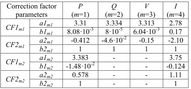
D. Calculation of the correction factors

Next, the two additional measurement sets are used to calculate the correction factors

CF1mn and CF2mn. The first point for both CF1mn and CF2mn curves is the base scenario,

while the case of a 5% step increase in the load power and of a 5% increase in the pre-disturbance steady state MG condition of the active and reactive power are considered as additional points for CF1mn and CF2mn, respectively. The calculated correction

factors are presented in Table 2.

According to the proposed modelling methodology, the model eigenvalues and phase parameters are considered constant and equal to the corresponding of the base scenario. The validity of the above assumptions is verified calculating the model parameters in detail for all examined disturbances. The mean value of the σmn parameters, normalized

with the corresponding base scenario value, is between 0.946 and 1.0117 with variance between 1.11·10-3 and 7.21·10-5. Considering the variance of the normalized ωmn and

φmn, the values are significantly low in the order of 10-4 to 10-6 with mean values close

to 1.

Table 2 Correction factor parameters Correction factor

parameters

P

(m=1)

Q

(m=2)

V

(m=3)

I

(m=4)

CF1m1 a1_b1m1 3.31 3.334 3.313 2.78

m1 8.08·10-3 8·10-5 6.04·10-3 0.17

CF2m1 a2m1 -0.412 -4.6·10

-2 _{-0.15 -2.10}

b2m1 1 1 1 1

CF1m2 a1_b1m2 3.383 - - 3.75

m2 -1.48·10-2 - - -0.124

E. Sensitivity analysis

Sensitivity analysis is applied to investigate the influence of each black-box model parameter on the MG dynamic responses and clarify the degree of accuracy required during the identification process. The normalized sensitivity functions are calculated using (10) with respect to the model parameter p under study (Amn, ωmn, σmn and φmn).

( ) ( )

( ) 

 



m

Y s m

p

m

Y s p

S

Y s p (10)

where Ym(s) is the Laplace Transform of ym(t) of (9). The normalized sensitivity in (10)

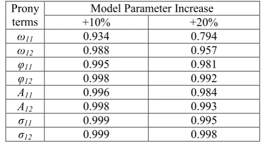
is a function of frequency, thus the suprema of all parameters in the frequency range of 0 Hz to 100 Hz are used in the comparisons. In all examined cases the suprema are located at a frequency close to the eigenfrequency of the corresponding Prony term. According to the calculated results, parameter ωmn presents the highest sensitivity, with

φmn, Amn and σmn following in order. Therefore, the accuracy of this parameter is of main

importance and stricter limits need to be specified as presented in Section 2. For this purpose, the initial estimation of ωmn using Prony analysis can be improved by applying

Fourier analysis.

Table 3 Active power R2 values for different model parameter variations. Prony

terms

Model Parameter Increase

+10% +20%

ω11 0.934 0.794

ω12 0.988 0.957

φ11 0.995 0.981

φ12 0.998 0.992

A11 0.996 0.984

A12 0.998 0.993

σ11 0.999 0.995

σ12 0.999 0.998

F. Model validation

Dynamic responses for the case of 15% step increase in the active and reactive power of the load and 15% increase in the pre-disturbance steady state MG condition of the active and reactive power are simulated, in order to validate the model accuracy. Dynamic responses are calculated using:

 detailed simulations without system reduction,

 the proposed model and its correction factors,

 Prony terms directly extracted from detailed results as in [20],

 parameters calculated by the base scenario (static load: 7.48 MW, 3 MVAr – 30% increase in the load).

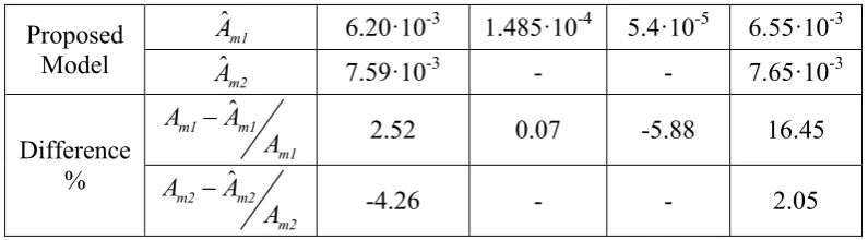
First, the resulting ˆ

mn

A parameters from (6) are compared in Table 4 with the

parameters extracted from the simulation data for the examined disturbance. The percentage difference is calculated using (11), where Amn are the extracted parameters

and ˆA_mnthe parameters derived from the proposed model.

ˆ

(%) mn mn 100

mn

A A

difference

A

  

_ _

  (11)

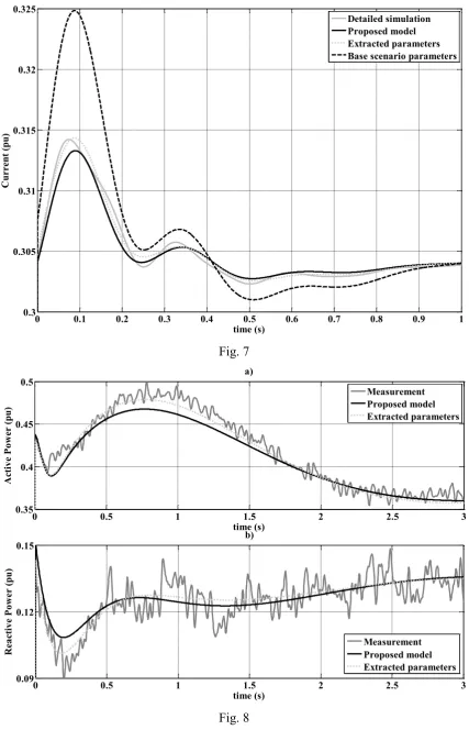
The dynamic responses of system variables P, Q and V, I are shown in Figs. 4-7, respectively. Results show a very good agreement between the proposed model and the detailed simulations. Differences between the proposed model parameters and the directly extracted, vary from 0.1 % up to 17 % as shown in Table 4, although the corresponding differences in the dynamic responses are generally smaller, as shown in Figs. 4 - 7. The results from the base scenario show the effect of Amn parameters on the

dynamic response amplitude. If only the initial measurement from the base scenario is used to extract the model parameters, significant errors may occur in the Amn

parameters, as shown in Figs. 4-7, highlighting the importance of the correction factors.

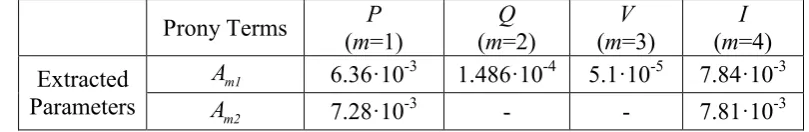
Table 4 Comparison of extracted and model parameters

Prony Terms _(mP _{=1) (m}Q _{=2) (m}V _{=3) (m}I ₌₄₎

Extracted Parameters

m1

A 6.36·10-3 1.486·10-4 5.1·10-5 7.84·10-3

m2

Proposed Model

ˆ m1

A 6.20·10-3 1.485·10-4 5.4·10-5 6.55·10-3 ˆ

m2

A 7.59·10-3 - - 7.65·10-3

Difference %

ˆ

m1 m1

m1

A A

A

 _{2.52 0.07 -5.88 16.45}

ˆ

m2 m2

m2

A A

A

 _{-4.26 - - 2.05}

[Fig. 4]

[Fig. 5]

[Fig. 6]

[Fig. 7]

A similar analysis is also conducted for TC1 and TC2. The system dynamics in TC1 are mainly related to the dynamic behaviour of DG1 and DG2, depending on the DG the disturbance is applied to, while in TC2 the inverter power output changes have a similar effect on the MG performance as in TC3.

In Table 5 the minimum and maximum errors are summarized for all system variables of each TC. The R2 values are calculated, assuming as reference the results of the detailed simulation, whereas the estimated responses are calculated using the proposed model. In all cases the results are in very good agreement, verifying the validity of the proposed model for different types of disturbances and MG operating conditions, with the worst R2 observed in TC3.

Table 5 Minimum and maximum R2 values for all examined test cases

Test cases min max

TC1 0.988 0.996

TC2 0.988 0.993

TC3 0.968 0.995

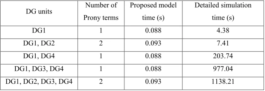
G. Simulation time

Finally, the computational efficiency of the proposed method is investigated, comparing the indicative simulation time, required for the calculation of dynamic responses in different MG configurations.

MATLAB/Simulink using an Intel Core 2 Duo E8400 processor at 3 GHz with 4GB of RAM. As shown in Table 6 in all cases the simulation time of the proposed model is less than 0.1 s, directly related to the number of the Prony terms involved in the modeling procedure. As expected, the computational efficiency of the proposed model increases with the number of the DG units involved in the MG configuration.

Table 6 Indicative simulation times.

DG units Number of

Prony terms

Proposed model time (s)

Detailed simulation time (s)

DG1 1 0.088 4.38

DG1, DG2 2 0.093 7.41

DG1, DG4 1 0.088 203.74

DG1, DG3, DG4 1 0.088 977.04

DG1, DG2, DG3, DG4 2 0.093 1138.21

4. Model evaluation with measurements

The analysis in the laboratory-scale MG test facility is mainly focused on disturbances caused by step load power increases in the MG operating in islanded mode to highlight the effect of frequency variations as well. Simulation and measurement responses are also presented for the grid-connected mode of operation, in order to validate the accuracy of the proposed model using measurement data sets under different operating conditions.

A. System under study

efficient hybrid method using the Clarke transformation and three single phase frequency locked loops is used, minimizing the ripple. No additional data processing is applied to the measurement data during the modelling procedure. Detailed information on the measurement algorithms is given in [30].

Sub-MG #1 consists of a 2 kVA synchronous generator (DG1), a 10 kVA inverter (DG2), a 10 kW/7.5 kVAr static load bank and a 2.2 kW, 0.87 lagging asynchronous machine. DG1 is driven by a dc motor emulating a fast-response prime mover. Both DG1 and DG2 follow a frequency-active power (f-P), voltage-reactive power (V-Q) droop control scheme, providing frequency and voltage support to the grid as ancillary services.

Sub-MG #2 consists of an 80 kVA synchronous machine (DG3) and a 40 kW/30 kVAr static load bank. DG3 is driven by a dc motor representing a slow-response prime mover. The control scheme followed is an f-P, V-Q droop control strategy and the generator can only operate in islanded mode, acting as a feeder and providing additional support to the voltage and frequency due to its large rated power.

B. Model development

The black-box model of Sub-MG #1 is developed from measurements for the islanded mode of operation, following the proposed methodology of Section 2. All system variables are recorded at Bus-3. The dynamic performance of the MG is affected by the droop controlled DG units of sub-MG #1, varying their power output during disturbances according to the corresponding slope.

In the base scenario DG1 is providing 1 kW/ 0.75 kVar and DG2 5 kW/ 3.75 kVar. The static load is 3.5 kW with power factor 0.8 lagging and the asynchronous motor is operating at its nominal power. A 40% increase is applied to the active and reactive power of the static load. All system variables are presented in pu with a base voltage of 400 V, base frequency 50 Hz and base power equal to 12 kVA.

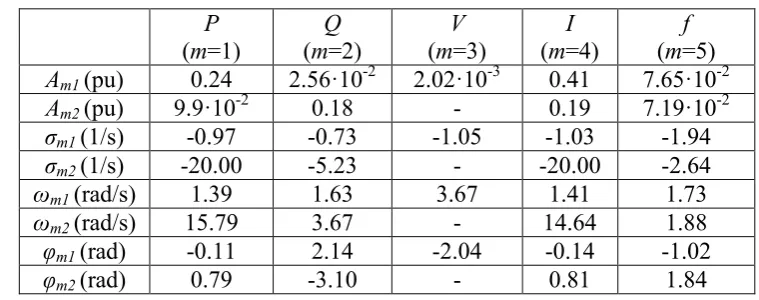
DG2. The bus voltage has a similar response to the reactive power but it is affected more by DG2. Finally, the system frequency response is represented by two Prony terms with similar oscillating frequencies but with different damping coefficients. This is due to the effect of DG3 on DG2, according to the corresponding f-P droop characteristic.

Table 7 Prony terms for the base scenario

P

(m=1) (mQ =2) (mV =3) (mI =4) (m=5)f

Am1 (pu) 0.24 2.56·10-2 2.02·10-3 0.41 7.65·10-2

Am2 (pu) 9.9·10-2 0.18 - 0.19 7.19·10-2

σm1 (1/s) -0.97 -0.73 -1.05 -1.03 -1.94

σm2 (1/s) -20.00 -5.23 - -20.00 -2.64

ωm1 (rad/s) 1.39 1.63 3.67 1.41 1.73

ωm2 (rad/s) 15.79 3.67 - 14.64 1.88

φm1 (rad) -0.11 2.14 -2.04 -0.14 -1.02

φm2 (rad) 0.79 -3.10 - 0.81 1.84

The two additional measurements required to calculate the model correction factors correspond to a 30% step increase in the load power and a different pre-disturbance steady state condition at 6.5 kW (30 % increase from the base scenario). Finally, the black-box model is developed, by introducing the calculated correction factors.

In order to evaluate the model performance a case where the Sub-MG #1 is driven to a new pre-disturbance steady state, is investigated with active and reactive power higher than 15% from the base scenario. Additionally, a disturbance caused by a 50% active and reactive load power increase is applied. Prony term parameters extracted directly from measurements and the corresponding using the proposed model are given in Table 8. In Figs. 8 and 9 measurement and simulation dynamic responses are compared, with Prony terms calculated using the proposed model and also directly extracted from the test data.

Table 8 Extracted parameters and parameters from the developed model

Prony Terms P

(m=1)

Q

(m=2)

V

(m=3)

I

(m=4)

f

(m=5) Extracted

Parameters

m1

A 0.27 2.4·10-2 2.26·10-3 0.45 9.05·10-2

m2

A 0.134 0.215 - 0.24 8.59·10-2

Model ˆ m2

A 0.131 0.201 - 0.25 8.51·10-2

Difference %

ˆ

m1 m1

m1

A A

A

 _{7.41 30.5 -8.9 -10.41 1.81}

ˆ

m2 m2

m2

A A

A

 _{1.95 -6.5 - 6.15 0.83}

[Fig. 8]

[Fig. 9]

Results show that the overall model performance is in good agreement with measurements. The RMSE and R2 for the different system variables varies from 1.88·10-4 up to 1.68·10-2and from 0.9873 up to 0.9412, respectively. Moreover, it is observed that higher errors in the Amn parameter estimation by the proposed model does

not necessarily lead to higher errors in the dynamic responses, since the corresponding eigenvalue may not be dominant in the MG response. This is the case mainly for the reactive power as shown in Table 8, where there is a -6.5% error in the A22 parameter,

corresponding to the faster and dominating eigenvalue and a 30.5% error in the A21

parameter, corresponding to the slower and less significant eigenvalue.

C. Application of the model on individual DG units

A black-box model is also implemented for the inverter interfaced DG2 unit of the examined laboratory test case. The proposed methodology is followed as in the case of the whole MG topology, using two Prony terms for both the active and reactive power. DG2 dynamic behaviour is affected by the system frequency and voltage variations, according to the corresponding f – P and V – Q droop characteristics. The active and reactive power dynamic responses are presented in Fig. 10 and are compared with measurements, showing good accuracy, since the RMSE and R2 are equal to 1.57·10-2 and 5.9·10-3, and 0.893 and 0.804 respectively. Therefore, the proposed model provides also the flexibility to implement black-box models of individual DG units, where detailed technical characteristics and parameters are unknown.

D. Application of the model in grid-connected mode of operation

The proposed model is also used for the case where Sub-MG#1 is grid-connected. All DG units and loads of Sub-MG#1 operate at the same conditions as in the islanded case, while Sub-MG#2 is disconnected. The results for the active and reactive power are shown in Fig. 11. The eigenfrequencies involved in the system dynamics are higher for the grid-connected operation compared to the islanded. For the active power only one term is needed and the dominating frequency is 3.3 Hz. Considering the reactive power two terms are required with frequencies 2.5 Hz and 27.8 Hz. The damping oscillations are identified more accurately leading to smaller differences between the proposed model parameters and the directly extracted and the corresponding R2 values range from 0.95 up to 0.98.

[Fig. 11]

5. Conclusions

A black-box dynamic MG model, based on Prony analysis is presented in this paper. The proposed model is suitable for the simulation of the dynamic responses of different MG system variables (P, Q, V, I and f), when subjected to internal disturbances. The disturbances include changes in the DG unit operating conditions and in the active and reactive power of the MG.

The model structure has a modular form and can be combined with power system simulation software platforms or used as a standalone analysis tool for power system dynamic studies. It has a generalized form, providing great flexibility in modelling a variety of MG systems with different degrees of complexity by adjusting the required terms without the need of prior knowledge of the MG topology. It can also be used to simulate individual DG units, eliminating the need to access the detailed parameters of the unit. The model incorporates a parameter calculation procedure, based on proper correction factors, which minimizes the need to update the model parameters after each disturbance thus improving significantly its numerical efficiency. Moreover, empirical guidelines are defined to help the parameter identification procedure.

performance of the proposed model. Different control strategies are investigated, including PQ and droop control schemes, in order to ensure the validity of the model for a wide range of operating conditions. The obtained results are in good agreement with the corresponding detailed simulations and real measurements, showing that the proposed model can be efficiently used in all types of MG systems.

6. References

[1] Jenkins N., Ekanayake J.B., and Strbac G.: "Distributed Generation" (IET, 2010).

[2] Katiraei F., Iravani R., Hatziargyriou N., and Dimeas A.: "Microgrids Management", IEEE Power and Energy Magazine, 6, (3), pp. 54-65, 2008. [3] Hatziargyriou N.D., Meliopoulos A.P.S.: "Distributed energy sources: technical

challenges", IEEEPower Engineering Society Winter Meeting, 2, pp.1017-1022, 2002.

[4] Annakkage U.D., Nair N.K.C., Liang Y., Gole A.M., Dinavahi V., Gustavsen B., Noda T., Ghasemi H., Monti A., Matar M., Iravani R., Martinez J.A.: "Dynamic System Equivalents: A Survey of Available Techniques", IEEE Trans. on Power Delivery, 27, (1), pp.411-420, Jan. 2012.

[5] Katiraei F., Iravani M.R., Lehn P.W.: "Small-signal dynamic model of a micro-grid including conventional and electronically interfaced distributed resources",

IET Generation, Transmission & Distribution, 1, (3), pp.369-378, May 2007. [6] Milanovic J.V., Kayikci M.: "Transient Responses of Distribution Network Cell

with Renewable Generation", PSCE '06, Atlanta, pp.1919-1925, 2006.

[7] Etemadi A.H., Davison E.J., Iravani R.: "A Decentralized Robust Control Strategy for Multi-DER Microgrids—Part I: Fundamental Concepts", IEEE Trans. on Power Delivery, 27, (4), pp.1843-1853, Oct. 2012.

[8] Trudnowski D.I.: "Order reduction of large-scale linear oscillatory system models", IEEE Trans. on Power Systems, 9, (1), pp.451-458, Feb 1994.

[10] Price W.W, Hargrave A.W., Hurysz B.J., Chow J.H., Hirsch P.M.: "Large-scale system testing of a power system dynamic equivalencing program", IEEE Trans. on Power Systems, 13, (3), pp.768-774, Aug 1998.

[11] Feng M., Vittal V.: "Right-Sized Power System Dynamic Equivalents for Power System Operation", IEEE Trans. on Power Systems, 26, (4), pp.1998-2005, Nov. 2011.

[12] Hussein D.N., Matar M., Iravani R.: "A Type-4 Wind Power Plant Equivalent Model for the Analysis of Electromagnetic Transients in Power Systems", IEEE Trans. on Power Systems, 28, (3), pp. 3096-3104, Aug 2013.

[13] Castro R.M.G., Ferreira De Jesus J.M.: "A wind park reduced-order model using singular perturbations theory", IEEE Trans. on Energy Conversion, 11, (4), pp.735-741, Dec 1996.

[14] Milanovic J.V., Mat Zali S.: "Validation of Equivalent Dynamic Model of Active Distribution Network Cell", IEEE Trans. on Power Systems, 28, (3), pp. 2101-2110, Aug 2013.

[15] Mat Zali S., Milanovic J.V.: "Generic Model of Active Distribution Network for Large Power System Stability Studies", IEEE Trans. on Power Systems, 28, (3), pp. 3126-3133, Aug 2013.

[16] Resende F.O., Pecas Lopes J.A.: "Development of Dynamic Equivalents for MicroGrids using System Identification Theory", PowerTech, 2007, Lausanne, pp.1033-1038, July 2007.

[17] Ning Z., Pierre J.W., Hauer J.F.: "Initial results in power system identification from injected probing signals using a subspace method", IEEE Trans. on Power Systems, 21, (3), pp.1296-1302, Aug. 2006.

[18] Feng X., Lubosny Z., Bialek J.W.: "Identification based Dynamic Equivalencing", PowerTech, Lausanne, pp.267-272, 1-5 July 2007.

[19] Hauer J.F.: "Application of Prony analysis to the determination of modal content and equivalent models for measured power system response", IEEE Trans. on Power Systems, 6, (3), pp.1062-1068, Aug 1991.

[21] t A.M., Saric A.T.: "Transient power system analysis with measurement-based gray box and hybrid dynamic equivalents", IEEE Trans. on Power Systems, 19, (1), pp.455-462, Feb. 2004.

[22] Roscoe A.J., Mackay A., Burt G.M., McDonald J.R.: "Architecture of a Network-in-the-Loop Environment for Characterizing AC Power-System Behavior", IEEE Trans. on Industrial Electronics, 57, (4), pp.1245-1253, April 2010.

[23] Hildebrand F.B., "Introduction to Numerical Analysis" (Dover Publications, 2nd Edition, 1987).

[24] Grund C.E., Paserba J.J., Hauer J.F., Nilsson S.: "Comparison of Prony and Eigenanalysis for Power System Control Design", IEEE Trans. on Power Systems, 8, (3), pp.964-971, August 1993.

[25] Katayama T.: ―Subspace Methods for System Identification‖ (Springer, 2005). [26] Matlab R2011b http://www.mathworks.com.

[27] Korunovic L.M., Sterpu S., Djokic S., Yamashita K., Villanueva S.M., Milanovic J.V.: "Processing of load parameters based on Existing Load Models", ISGT Europe, 14-17 Oct. 2012.

[28] Papadopoulos P.N., Chatzisideris M.D., Papadopoulos T.A., Marinopoulos A.G., Papagiannis G.K.: "Integration of Smart Grid Technologies in a MicroGrid with PV and FC units", UPEC 2011, Soest Germany, 5-8 Sept. 2011. [29] Papadopoulos P.N., Papadopoulos T.A., Papagiannis G.K.: "Dynamic modeling

of a microgrid using smart grid technologies", UPEC 2012, London 4-7 Sept. 2012.

Figure Captions

Fig. 1: Black-box modelling procedure flowchart.

Fig. 2: Amplitude parameter of Prony term against the disturbance amplitude and the MG operating condition.

Fig. 3: MG systems under study for a) simulations and b) measurements. Fig. 4: Dynamic response of the active power.

Fig. 5: Dynamic response of the reactive power. Fig. 6: Dynamic response of the bus voltage. Fig. 7: Dynamic response of the current.

Fig. 8: Responses of the a) active and b) reactive power.

Fig. 9: Responses of the a) bus voltage, b) current and c) frequency. Fig. 10: Responses of the a) active, b) reactive power of the inverter.

Step 1 Record 3 datasets

Step 2 Prony analysis

Step 3

Nonlinear least square optimization

Step 4 Correction factors calculation

Step 5 Black-box model

formulation Empirical

guidelines

RMSE < target, R-square > target

Repeat

YES NO

Update initial values and boundaries

Fig. 1

5

10

15

20

25

30

0 5 10 15 20 25 300 0.2 0.4 0.6 0.8 1

disturbance amplitude increase % initial point increase %

A

m

pl

itude

pa

ra

m

eter

(pu)

PV DG1

5 MVA

20 kV MV BUS

External Grid 250 MVA PCC AC DC DG2

2 MVA _FC

AC

DC

DG3

0.58 MW 1 MWDG4

1.2 MVA 0.7 MVA Static Load 7.48 MW, 3 MVAr Microgrid DG1 2 kVA Static Load 10 kW 7.5 kVAr DG2 AC DC G M Sub-MG #1 10 kVA Bus-4 G Bus-3 DG3 80 kVA Static Load 40 kW 30 kVAr Utility Supply 500 kVA Bus-1 Bus-2 Sub-MG #2 Dynamic Load 2.2 kW L1 S2 PCC S1 S3 a) b) Fig. 3

0 0.1 0.2 0.3 0.4 0.5 0.6 0.7 0.8 0.9 1

-0.235 -0.23 -0.225 -0.22 -0.215 -0.21 time (s) A cti ve P ow er (pu) Detailed simulation Proposed model Extracted parameters Base scenario parameters

0 0.1 0.2 0.3 0.4 0.5 0.6 0.7 0.8 0.9 1 -0.213

-0.207 -0.201 -0.196

time (s)

R

ea

cti

ve

po

w

er

(pu)

Detailed simulation Proposed model Extracted parameters Base scenario parameters

Fig. 5

0 0.1 0.2 0.3 0.4 0.5 0.6 0.7 0.8 0.9 1

0.9908 0.9915 0.9921

time (s)

V

ol

ta

ge

(pu)

Detailed simulation Proposed model Extracted parameters Base scenario parameters

0 0.1 0.2 0.3 0.4 0.5 0.6 0.7 0.8 0.9 1 0.3

0.305 0.31 0.315 0.32 0.325

time (s)

C

urrent

(pu)

Detailed simulation Proposed model Extracted parameters Base scenario parameters

Fig. 7

0 0.5 1 1.5 2 2.5 3

0.35 0.4 0.45

0.5 a)

time (s)

A

cti

ve

P

ow

er

(pu)

0 0.5 1 1.5 2 2.5 3

0.09 0.12

0.15 b)

time (s)

R

ea

cti

ve

P

ow

er

(pu)

Measurement Proposed model Extracted parameters

Measurement Proposed model Extracted parameters

0 0.5 1 1.5 2 2.5 3 0.989 0.991 0.993 0.9949 a) time (s) V ol ta ge (pu)

0 0.5 1 1.5 2 2.5 3

0.65 0.75 0.85 0.95 b) time (s) C urrent (pu)

0 0.5 1 1.5 2 2.5 3

0.994 0.996 0.998 1 1.002 c) time (s) F requency (pu) Measurement Proposed model Extracted parameters Measurement Proposed model Extracted parameters Measurement Proposed model Extracted parameters Fig. 9

0 0.5 1 1.5 2 2.5 3

0.45 0.5 0.55 0.6 0.65 a) time (s) A cti ve P ow er (pu)

0 0.5 1 1.5 2 2.5 3

0 0.1 0.2 0.3 0.4 0.5 0.6 0.7 0.8 0.9 1 0.38

0.39 0.4 0.41 0.42 0.43

0.44 a)

time (s)

A

cti

ve

P

ow

er

(pu)

0 0.1 0.2 0.3 0.4 0.5 0.6 0.7 0.8 0.9 1

0.06 0.07 0.08 0.09

0.1 b)

time (s)

R

ea

cti

ve

P

ow

er

(pu)

Measurement Proposed model Extracted parameters

Measurement Proposed model Extracted parameters