Simulation of incompressible viscous flows around moving objects by a variant of immersed boundary-Lattice Boltzmann method

Simulation of Incompressible Viscous Flows around

Moving Objects by A Variant of Immersed

Boundary-Lattice Boltzmann Method

J. Wu, C. Shu1

Department of Mechanical Engineering, National University of Singapore 10 Kent Ridge Crescent, Singapore 119260

and Y. H. Zhang

Department of Mechanical Engineering, University of Strathclyde, Glasgow, G1 1XJ, UK

Abstract

A variant of immersed boundary-lattice Boltzmann method (IB-LBM) is presented in this paper to simulate incompressible viscous flows around moving objects. As compared with the conventional IB-LBM where the force density is

computed explicitly by the Hook’s law or the direct forcing method and the non-slip condition is only approximately satisfied, in the present work, the force density term is considered as the velocity correction which is determined by enforcing the non-slip condition at the boundary. The lift and drag forces on the moving object can be easily calculated via the velocity correction on the boundary points. The capability of present method for moving objects is well demonstrated through its application to

1

simulate flows around a moving circular cylinder, a rotationally oscillating cylinder, and an elliptic flapping wing. Furthermore, the simulation of flows around a flapping flexible airfoil is carried out to exhibit the ability of present method for implementing the elastic boundary condition. It was found that the flapping flexible airfoil can generate larger propulsive force than the flapping rigid airfoil.

1. Introduction

In recent years, the study on interaction between fluid and moving objects receives more and more attention as moving boundary problems are often appeared in the study of fish motion, insect flight, blood flow through heart valves, and countless others. Simulation of flows around moving objects accurately and efficiently puts a great challenge to numerical techniques, and is currently at the forefront in the computational fluid dynamics.

The numerical approaches for simulation of flows around moving objects can be roughly classified into two major categories, boundary conforming methods and

part of objects moves locally with a different mode, the multi-block time-dependent coordinate transformation, which could be very tedious, has to be applied. To consider the general moving boundary problem, Li et al. [5] proposed the moving mesh finite element algorithm, in which re-meshing and interpolation are needed. Perhaps, the most popular boundary conforming method is the arbitrary Lagrangian Eulerian (ALE) approach [6-11], which is normally applied with finite difference, finite volume and finite element schemes. Due to regenerating the mesh to conform to the boundary at all times, it becomes difficult for ALE approach to solve the moving boundary problems with complex geometry, especially for the three-dimensional problem. In the category of non-boundary conforming methods, the governing equations are solved on a fixed Cartesian grid, and the boundary no longer coincides with the grid surface. The effect of boundary is accounted through the proper treatment of the solution variables at grid cells around the boundary. As compared to the boundary conforming methods, the non-boundary conforming methods eliminate the

requirement of tedious grid adaptation, which makes the simulation of flows around complex boundaries undergoing movement be more straightforward.

structures of the cut cells, the calculation of fluxes at the interface of cut cells requires complicated treatment, which may bring inconvenience and affect the computational efficiency. Recently, Zhou et al. [17] proposed an efficient Cartesian grid method, namely, the local domain-free discretization (DFD) method, for simulation of compressible flows around moving boundaries. In the local DFD method, the boundary information is transferred to an adjacent point to the boundary through low order interpolation.

The immersed boundary method (IBM) may be the simplest non-boundary conforming method. It has been firstly proposed by Peskin [18] in the 1970s when he studied the blood flow in the human heart. Since then, numerous modifications and refinements have been proposed and a number of variants of this approach were proposed [19-22]. In the IBM, the flow field is represented by a set of Eulerian points, which are in fact the fixed Cartesian mesh points, and the boundary of immersed object is represented by a set of Lagrangian points. The basic idea of IBM is to treat

standard LBM is usually applied on the Cartesian mesh. Due to this common feature, it is desirable to combine these two methods together. Many efforts [24-26] have been made in this aspect.

One of key issues in the application of IBM is the computation of restoring force. Basically, there are three ways. The popular way is the penalty method [18], in which the Hook’s law is applied, and the spring parameter needs to be specified by the user. The second way is called the direct forcing method, which has been introduced firstly by Fadlun et al. [27]. This way directly applies the momentum equations at the boundary points to compute the force density. The third way has been proposed by Niu et al [28], in which the momentum exchange at the boundary is used to compute the force. It is noted that all the three ways compute the restoring force explicitly. As pointed out by Shu et al. [29], the pre-calculated restoring force cannot guarantee that the corrected velocity field due to presence of immersed boundary satisfies the non-slip condition at the boundary. As a result, obvious flow penetration to the

immersed boundary can be observed in the IBM results. Flow penetration implies mass exchange across the boundary. As we know, mass exchange would bring the momentum exchange, leading to a numerical force. Clearly, this force error will affect the accuracy of lift and drag forces acting on the immersed object. This greatly limits the application of IBM to the moving boundary problems.

Boltzmann method. In the present work, the restoring force is determined by enforcing the non-slip condition on the boundary. Since the non-slip condition is accurately satisfied, no flow penetration can be found in the present results. Due to this improvement, it is expected that the present approach can be well applied to simulate flows around moving objects. The flows around a moving circular cylinder, a rotationally oscillating cylinder, and an elliptic flapping wing are chosen to validate the present approach. The obtained results agree very well with available data in the literature. Furthermore, the flow around the flapping flexible airfoil is simulated to exhibit the ability of present approach for implementing the elastic boundary condition.

2. Numerical method

2.1 Conventional immersed boundary method

In the immersed boundary method, the effect of boundary to the surrounding fluids is through a force density exerting on them. The governing equations of

immersed boundary method for the viscous incompressible flows can be written as

p t

ρ⎛_⎜∂ + ⋅∇ + ∇ = Δ +⎞_⎟ μ

∂

⎝ ⎠

u _{u u u f}

(1)

0

∇ ⋅ =u (2)

( )

( )

(

( )

)

=

∫

( )

₍

_{( )}

₎

_{( )}

₍

_{( )}

₎

, , , ,

s t

s t t t s t d

t Ω δ

∂

= = −

∂

∫

X

u X u x x X x (4)

where x, u and f are the Eulerian coordinate, fluid velocity and force density acting on the fluid, respectively, p is the fluid pressure, ρ is the fluid density and

μ is the dynamic viscosity. X and F represent Lagrangian coordinates and

boundary force density. δ

(

( )

)

are the N-S equations with external force. Equations (3)-(4) describe the interaction between the immersed boundary and the fluid flow by distributing the boundary force at the Lagrangian points to Eulerian points and interpolating the velocity at the Eulerian points to Lagrangian points. The calculation of boundary force density F,

which is also called restoring force, is critical in the IBM. Using Hooke’s law, it can be determined by

( )

(

)

F V V (5)

where V_fluid is the fluid velocity at the boundary point interpolated from the

surrounding fluid (Eulerian) points, V_wall is the boundary velocity of the object, k is

the spring coefficient. Note that the boundary force density can also be computed by the direct forcing method [27] and the momentum exchange method [28]. The basic solution process of IBM can be summarized as follows:

(1) Set force density f as zero at beginning. Solve equations (1) and (2) to get flow variables at Eulerian points;

(2) Interpolate velocity at Eulerian points to the boundary (Lagrangian) points by using equation (4);

object to compute the boundary force density F by using equation (5); (4) Compute the force density f at Eulerian points by using equation (3);

(5) Solve equations (1) and (2) with the force density f to get the corrected velocity field at Eulerian points;

(6) Go back to step (2) until the convergence criterion is satisfied.

It should be noted that in the above process, when the boundary force F, and therefore the force density f, is computed explicitly, the new (corrected) velocity given in step (5) may not satisfy the non-slip boundary condition. So, IBM needs to continue the process until convergence state is reached, and hopes that at the converged state, the non-slip condition can be satisfied. However, we have to indicate that in the whole process, there is no guarantee to satisfy the non-slip boundary condition. Indeed, it is only approximately satisfied. This could be the major reason to cause flow penetration to the solid body in the conventional IBM results. As shown in the following section, we will present a variant of IB-LBM to enforce the non-slip boundary condition.

2.2 A Variant of immersed boundary-lattice Boltzmann (IB-LBM) method

Equations (1) and (2) are the governing equations for the flow field. In the lattice Boltzmann context, they can be replaced by the lattice Boltzmann equation. In this work, the form of lattice Boltzmann equation proposed by Guo et al. [30] is adopted, which can be written as

(

)

( )

(

( )

( )

)

, , , eq ,

f_{α α}δt t δt f_α t f_α t f_α t F_α t

τ δ

+ + − = − − +

2 4 1

1

2 _{s s}

F w

c c

α α

α α α

τ

− ⋅

=⎛_⎜ − ⎞_⎟ ⎛_⎜ + ⎞_⎟⋅

⎝ ⎠ _{⎝ ⎠}

e u e u

e f (7)

1

2

f t

α α α

ρu=

∑

where f_α is the distribution function, f_αeq is its corresponding equilibrium state, τ is the single relaxation time, e_α is the particle velocity, w_α are coefficients which

depend on the selected particle, and f is the external force density. For the popular D2Q9 model [31], the particle velocity set is given by

(

)

(

)

(

)

(

)

(

)

(

)

0 0

cos 1 2 , sin 1 2 1, 2, 3, 4

2 cos 5 2 4 , sin 5 2 4 5, 6, 7,8

c

c

α

α

α π α π α

α π π α π π α

⎧ ₌ ⎪ ⎪ =_⎨ ⎡_⎣ − ⎤_⎦ ⎡_⎣ − ⎤_⎦ = ⎪ − + − + = ⎡ ⎤ ⎡ ⎤ ⎪ _{⎣ ⎦ ⎣ ⎦} ⎩ e (9)

where c=δ δx t, δx and δt are the lattice spacing and time step, respectively.

The corresponding equilibrium distribution function is

( )

(

)

(

)

f t w

c c

α α

α ρ α

⎡ _{⋅ ⋅ −} ⎤

⎢ ⎥

= + +

⎢ ⎥

⎣ ⎦

e u u

e u

x (10)

with w₀ =4 9, w₁=w₂ =w₃=w₄=1 9 and w₅ =w₆=w₇ =w₈ =1 36 . c_s =c 3

is the sound speed of this model. The relation between the relaxation time and the

kinematic viscosity of fluid is 1 2 2 cs t υ=⎛_⎜τ − ⎞_⎟ δ

⎝ ⎠ . If we define the intermediate velocity

*

u as f

α α α

ρ_u∗₌

_∑

(11) and the velocity correction as

1

2 t

ρδu= fδ (12)

u u= ∗+δu (13)

In the conventional IB-LBM, f is computed explicitly by equation (5) or the direct forcing method [25, 27] or the momentum exchange method [28]. When the corrected velocity field is obtained from equation (13), there is no guarantee that the velocity at the boundary point interpolated from the corrected velocity field satisfies the non-slip boundary condition. To overcome this drawback, we have to consider the force density f as unknown, which is determined in such a way that the velocity at the boundary point interpolated from the corrected velocity field satisfies the non-slip boundary condition. As shown in Fig. 1, the velocity correction δu at Eulerian points is distributed from the velocity correction at the boundary (Lagrangian) points. In the IBM, the boundary of the object is represented by a set of Lagrangian points

( )

B s t

X ,l=1, 2,",m. Here, we can set an unknown velocity correction vector l B

δu

at every Lagrangian point. The velocity correction δu at the Eulerian point can be obtained by the following Dirac delta function interpolation

( )

(

)

(

( )

)

u t u X_{B B} t x X_B s t ds

δ δ δ

Γ

=

∫

In the actual implementation, δ

(

( )

)

( )

(

)

(

) (

) (

)

δ x X− = x −X =δ − δ − (15)

where δ

( )

( )

(

( )

)

0, 2 r r r r π

δ _{= ⎨}⎧⎪ + ≤

⎪ >

⎩

(16)

( )

(

) (

)

l

t t D s

δu x =

∑

(

)

where Δs_l is the arc length of the boundary element. In order to satisfy the no-slip

boundary condition, the fluid velocity at the boundary point must be equal to the boundary velocity at the same position

(

)

( ) (

)

,

, ,

l l l

B B ij ij ij B i j

t =

∑

U X u x x X ₍₁₈₎

Here, Ul_B is the boundary velocity; u is the fluid velocity, which is corrected by

the velocity correction δu

( )

( )

δ

( )

u x u x u x (19)

where u∗ is the intermediate fluid velocity obtained from equation (11). Note that the unknowns in equations (18) and (19) are the velocity corrections at the boundary points, l

B

δu . Substituting equations (19) and (17) into equation (18) gives

(

)

( ) (

)

(

) (

)

(

)

l l l

B B ij ij ij B

i j

l l l l

B B ij ij B l ij ij B i j l

t t D

t D s D

x y

x y

δ ∗

= −

− Δ −

Δ Δ

+

Δ Δ

∑

∑∑

U X u x x X

u X x X x X (20)

Equation system (20) can be further rewritten as the following matrix form =

AX B (21)

where X=

{

}

{

}

(

)

( )

(

)

,

, ,

l l l

l B B ij ij ij B

i j

t ∗ t D

x y

Δ =u U X −

∑

Δ Δ

(

)

f_α

α

ρ =

∑

s

P=c ρ ₍₂₃₎

With velocity correction δu, the force density f can be simply calculated by equation (12) as

2ρδ δt

=

f u (24)

Equation (24) can be applied at the boundary points to compute the lift and drag forces. The basic procedure of present IB-LBM is outlined as follows,

‹ Step 1: Set initial values, compute the elements of matrix A and get its inverse

matrix _A−1 ;

‹ Step 2: Use equation (6) to get the density distribution function at time level

n

t=t (initially setting F_α =0) and compute the macro variables using equations

(11) and (23);

‹ Step 3: Solve equation system (21) to get the velocity corrections at all boundary

points and use equation (17) to get velocity corrections at Eulerian points;

‹ Step 4: Correct the fluid velocity at Eulerian points using equation (19) and

obtain the force density using equation (24);

‹ Step 5: Compute the equilibrium distribution function using equation (10); ‹ Step 6: Repeat Step 2 to Step 5 until convergence is reached.

3. Results and discussion

3.1 Steady flow over a stationary circular cylinder

the steady flow over a stationary circular cylinder is selected for simulation. This problem has been studied extensively and there are numerous theoretical, experimental, and numerical results available in the literature. Depending on the Reynolds number, different kind of flow behaviors can be characterized. Here, the Reynolds number is defined as

Re U D

υ∞

= (25)

where U_∞ is the free stream velocity, D is the diameter of cylinder, and υ is the

kinematic viscosity.

It has been pointed out by Lai and Peskin [33] that, the drag force arises from

two sources: the shear stress and the pressure distribution along the body. The drag

coefficient is defined as

( )

1 2

D d

F C

U D

ρ _∞

= ₍₂₆₎

where F_D is the drag force. Here, it can be calculated by

D x

F f d

Ω

= −

_∫

x

f stands for the x-component of force density f at the boundary point.

The simulations at Re = 20 and 40 are carried out. The computational domain is

set by 50D×50D with a mesh size of 451×401. The cylinder is located at (20D,

25D). The free stream velocity is taken as U_∞ =0.1 and the fluid density is ρ =1.0.

The computation starts with the given free stream velocity. At the far field boundaries,

the equilibrium distribution functions are used to implement the boundary condition.

To well capture the accurate solution near the cylinder surface, fine grid should be

coarse grid is good enough for the region far away from the cylinder. To balance these

two, the non-uniform mesh is used in the present simulation. As the standard lattice

Boltzmann method is only applicable on the uniform mesh, in this work, we adopt the

Taylor series expansion and least squares-based lattice Boltzmann method (TLLBM)

[34], which can be well applied on the non-uniform mesh. The region around the

cylinder is 1.2D×1.2D with a very fine uniform mesh size of 97×97.

The streamlines are plotted in Fig. 2 for the case of Re = 40. As shown in the

figure, a pair of symmetric recirculation bubbles appears in the wake of the cylinder.

At the same time, we can observe two pairs of weak vortices enclosed inside the

cylinder. It means that the flow inside the cylinder has been occluded by the boundary.

This is an ideal case as it ensures no mass exchange between interior and exterior of

the cylinder surface. To the best of our knowledge, this is the first such promising

result obtained by IBM and its various versions. The good performance of present

results is indeed due to enforcement of non-slip boundary condition to prevent flow

penetration to the boundary.

Table 1 compares the length of recirculation bubbles L (based on the diameter of

cylinder D) and drag coefficients C_d for two cases with previous data [35-37]. Also

shown in the table are the results obtained by conventional IB-LBM [28]. From the

table, we can see clearly that the present drag coefficients are closer to the

experimental data and numerical results obtained by body-fitted N-S solvers than the

conventional IB-LBM results. This is also because the non-slip boundary condition is

the boundary force could be computed more accurately. This is of underlying

importance for moving boundary flow problems.

3.2 Flow over a moving circular cylinder

For the case presented above, the cylinder is stationary. To investigate the

capability of present method for modeling moving boundary flow problems, the

simulation of flow over a moving cylinder is carried out. To ease the simulation, the

uniform mesh is used. For making comparison, the flow over a stationary cylinder is

also simulated on the same mesh. The computational domain is set by 32D×32D

with a mesh size of 1281×1281. The stationary cylinder is located at (8D, 16D). The

moving cylinder moves towards the left from the position of (30D, 16D). The

Reynolds number for both case are taken as Re = 40.

To compare the results of moving cylinder case with that of stationary cylinder

case, we can adjust the frame of reference. It can be easily implemented by adding an

opposite velocity U_∞ onto the velocity in the Eulerian mesh. The adjusted

streamlines are shown in Fig. 3. For comparison, the streamlines of stationary

cylinder case are also shown in Fig. 3. It is apparent that the results of both cases have

good agreement with each other. The good agreement of both results can be further

confirmed by Fig. 4, which compares the pressure profiles on the surface of cylinder

for two cases. Through this example, on one hand, we demonstrate the capability of

present method for simulation of flows around a moving object; on the other hand, we

3.3 Flow over a rotationally oscillating cylinder

Vortex shedding in the near wake behind a bluff body could produce periodically

oscillating drag and lift forces. These fluctuating forces would produce structural

vibrations, acoustics noise or resonance. Hence, it is very important from practical

engineering perspective to control vortex shedding appropriately. Many attempts for

such control have been made recently. One of simple attempts is the rotary control of

cylinder wake [38, 39]. Here, we apply our developed method to simulate such

moving boundary flow problem.

The control of motion has the form of the rotary oscillation of the cylinder with

the instantaneous rotational velocity given by

( )

(

)

2

sin 2 U sin 2 St_f U

t ft A t

D D

γ ₌γ π ₌ ∞ ⎛ π ∞ ⎞

⎜ ⎟

⎝ ⎠ (28)

where U_∞ and D represent the free stream velocity and diameter of cylinder, respectively. f and γ₀ are the frequency and the rotation amplitude respectively,

which can be expressed in terms of non-dimensional parameters: the Strouhal number St_f = fD U_∞and the normalized amplitude A=γ₀D

(

)

are sufficient to characterize the control.

The computational domain is set by 50D×40D and the cylinder is located at (20D, 20D). The region around the cylinder is 1.2D×1.2D with a very fine uniform mesh size of 121×121. The whole domain is discretized on the non-uniform mesh. Hence, the TLLBM [34] is applied.

and diameter of cylinder D, the Reynolds number is taken as Re = 100. To verify our method for this problem, the case of Stf = 0.163 is simulated firstly. At Re = 100, the natural vortex shedding (Stn) for flow over a stationary cylinder is about 0.163. As indicated by Choi et al. [38], when Stf = Stn, the interesting vortex shedding pattern would happen, which is shown in Fig. 5. Note that the result of Choi et al. [38] is also included in Fig. 5 for comparison. It is clear from the figure that the present result compares well with that of Choi et al [38]. We also simulate the case of Stf = 0.4 to compare the forces exerted on the cylinder with that of Choi et al [38]. The obtained time-averaged coefficient and maximum amplitude of lift coefficient fluctuation are 1.302 and 0.321 respectively, which have good agreement with 1.231 and 0.299 from [38].

After verification of the method, the cases for five different forcing frequencies are simulated. They are Stf = 0.1, 0.16, 0.3, 0.7, and 0.9. Figure 6 illustrates the instantaneous vorticity contours obtained from the numerical simulations at the same

the wake of the cylinder. In Fig. 6 (e), the near-wake structure also becomes synchronized with the forcing. However, it becomes unstable and merges into a large-scale vortex some distance downstream. In Fig. 6 (f), the oscillation forcing only generates small-scale vortices in the shear layers near the cylinder, and most of the wake resembles that behind the stationary cylinder.

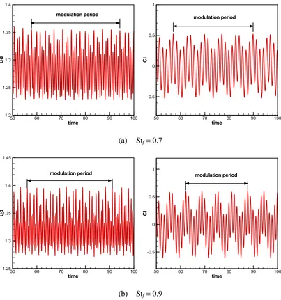
The flow behind a rotationally oscillating cylinder can be classified into two categories: lock-on and non lock-on. According to Choi et al. [38], the cases for Stf being equal to 0.1, 0.16, and 0.3 belong to lock-on and the remaining cases belong to non lock-on. As pointed out in [38], one of the characteristics for the non lock-on region is the occurrence of modulation phenomenon. The modulation frequency is very low as compared to the forcing and vortex shedding frequencies. Figure 7 shows the time histories of the lift and drag coefficients for non lock-on cases. Figure 8 shows the variations of the time-averaged drag coefficients and the maximum amplitude of the lift coefficient fluctuations due to the rotary oscillation forcing. In

the present simulation, the mean drag coefficient for the stationary cylinder is about 1.361. It is shown in Fig. 8 (a) that the mean drag decreases markedly with increasing Stf in the lock-on region, and it increases gradually with increasing Stf in the non lock-on region. The local minimum of mean drag exists near the boundary between the lock-on and non lock-on regions. The similar trend is found for the maximum amplitude of the lift coefficient fluctuations in Fig. 8 (b).

The flapping insect flight has fascinated physicists and biologists for more than one century. As compared to the fixed wing, flapping wing demonstrates attractive lift enhancement due to unsteady effects, which is very important for insect flight. Using the proposed method, we will simulate unsteady flows arising from flapping of a single elliptical wing to display the flow patterns associated with wing translation and rotation, as well as stroke reversal. The obtained fluid forces on the object are compared with those obtained numerically and experimentally in References [40] and [41].

In current simulation, the elliptical wing of aspect ratio 10 follows a prescribed sinusoidal translational and rotational motion. Specially, the wing sweeps in the horizontal plane and pitches about its center

( )

A

x t = π ft , y t

( )

( )

(

)

α =α +β π +φ (30)

where x t

( ) ( )

( )

which is measured counterclockwise relative to the positive x-axis. The parameters also include the stroke amplitude A₀, the initial angle of attack α₀, the amplitude of pitching angle of attack β, the frequency f and the phase difference φ between

( )

x t and a t

( )

between rotation and translation is a critical parameter in force generation. Here, two phase differences are selected: φ π= 4 and −π 4, corresponding to the advanced

and delayed rotation, respectively. To make a fair comparison, all above parameters are chosen the same as those used by Wang et al. [40] and Eldredge [41]. The computational domain of 20c×20c is discretized by a non-uniform mesh. The region around the center of domain for the wing motion is 3.5c×1.2c with a very fine uniform mesh size of 281×97.

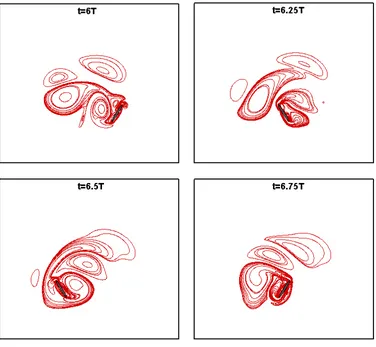
Figure 9 shows four snapshots of vorticity contours given in one cycle for advanced rotation of φ π= 4. They are very similar to those obtained by Eldredge

[41], which gave the physical interpretation.

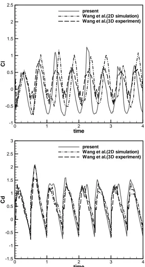
The time histories of lift and drag coefficients are plotted in Fig. 10. The previous numerical and experimental results [40, 41] are also included for comparison. All forces are normalized by the maxima of the corresponding quasi-steady forces which are mentioned in [40]: C_L =1.2 sin 2

( )

( )

the angle of attack. From Fig. 10, we can see that the present lift coefficient matches very well with the result of Eldredge [41], and the peak values are in good agreement with those from Wang et al. [40] in the whole four strokes. In the later strokes, the peak values of lift also compare well with experimental results of [40]. The present drag coefficients also agree very well with those given in [40-41]. Figure 11 depicts the vorticity contours for the delayed rotation case of φ= −π 4. By comparing the results of φ π= 4 with those of φ= −π 4, the sensitivity to the kinematics is

recaptured and trailing edge vortex shedding is also observed. The instantaneous lift and drag coefficients are plotted in Fig. 12 and are compared with those of Wang et al [40]. It can be found that the agreement is reasonable. By comparing Fig. 10 with Fig. 12, we can find that the characteristics of lift and drag are very different. The time-averaged lift and drag coefficients are (0.526, 0.567) and (0.101, 0.721) respectively for advanced and delayed rotation cases. From these values, we can conclude that the phase difference φ affects the force generation significantly,

especially for the lift production.

3.5 Flow over a flapping flexible airfoil

The numerical solution of fluid flow problems with thin flexible moving objects is motivated by the wide range of potential applications in biology and physiology. To exhibit the capability of our method for modeling such problems, the simulation of a single flapping flexible airfoil is carried out.

In our simulation, a single NACA0012 airfoil with flexural deformation executes plunge motion, which means that the airfoil makes the cross flow oscillation. The plunge motion of airfoil shown in Fig. 13 can be expressed by

( )

h=h c ωt (31)

where h means the instantaneous position of the airfoil, h₀ is the dimensionless

stroke amplitude, c denotes the chord length of the airfoil, and ω is the flapping

frequency.

airfoil varying over time can be expressed by

(

)

2

0 cos

y= −a cx ω φt+ (32)

where a₀ is the dimensionless flexure amplitude and

φ

the above equation, the x-y local frame refers to the body coordinate system and x is in the range of

[ ]

the tail.

In current study, the parameters for controlling the airfoil motion are chosen as:

0 0.4

h = , a₀ =0.3, φ π= 2, and

ω

based on the chord length c is Re = 500. A non-uniform mesh is used in the whole

computational domain of 30c×24c. In the small region around the airfoil (1.1c×1.5c) where airfoil is moved, a very fine uniform mesh size of 221×301 is applied.

The instantaneous vorticity contours in one cycle and evolution of drag coefficient are plotted in Fig. 14 and 15, respectively. For comparison, the results of flapping rigid airfoil with the same stroke amplitude are also included. In both cases, the flapping frequency ω is 0.4. From Fig. 14, we can observe the vortex being shed

Additionally, it is noticeable in Fig. 15 that the maximum of negative drag coefficient for flexible airfoil is much larger than that of rigid airfoil, and that more negative drag region appears for flapping flexible airfoil. Therefore, it may be concluded that the flexure could effectively augment the propulsive force for flapping airfoil.

Figure 16 presents the evolution of the pressure contours around the rigid and flexible airfoils during one cycle. The corresponding results for the lift coefficients are plotted in Fig. 17. As can be seen from Fig. 16, the pressure in the wake of flexible airfoil is higher than that of rigid airfoil. As a result, the pressure contributes less drag force for the flexible airfoil case. This is in line with the findings in [42].

To demonstrate the effect of flapping frequency on the generation of thrust force, the evolution of drag coefficients with four different flapping frequencies is depicted in Fig. 18. It is clear that the maximum negative drag coefficient increases with the flapping frequency. Higher frequency implies more generation of propulsive force.

Let T denote the flapping period, the period-averaged thrust force F_x can be

calculated by

( )

x x

F F t dt

T

=

_∫

where F t_x

( )

to the negative drag force. Therefore, we can define the period-averaged thrust power coefficient ξ as

(

)

2 1 T x d F U C dt T

U c U

ξ ρ

∞

∞ ∞

= = −

∫

frequency. Hence, same conclusion with that from Fig. 18 can be obtained.

4. Conclusions

A new version of immersed boundary-lattice Boltzmann method (IB-LBM) is presented in this paper for simulating incompressible viscous flows around moving objects. In the conventional IB-LBM, the force density is calculated explicitly by the Hook’s law or the direct forcing method or the momentum exchange method. Therefore, the non-slip boundary condition is only approximately satisfied. In this study, the force density, which can be recognized as the velocity correction, is set as unknown. It is solved by enforcing the non-slip boundary condition. Moreover, the lift and drag forces on the moving object can be easily calculated via the velocity correction on the boundary points. The lattice Boltzmann equation with a force density term is adopted in this work to obtain the flow field on the Eulerian points.

To show that the present method does not have any flow penetration to the solid boundary and provides better results for the forces acting on the object, the steady

airfoil, the flapping flexible airfoil can easily generate the propulsive force. Through numerical experiments, it is believed that the present method has a potential to effectively simulate incompressible viscous flows around moving objects.

References

1. K. Tsiveriotis and R. A. Brown, Boundary-Conforming Mapping Applied to Computations of Highly Deformed Solidification Interfaces, Int. J. Numer.

Methods Fluids, 14, 981-1003 (1992).

2. D. Mateescu, A. Mekanik, and M. P. Païdoussis, Analysis of 2-D and 3-D Unsteady Annular Flows with Oscillating Boundaries, Based on a

Time-Dependent Coordinate Transformation, J. Fluids Struct. 10 , 57–77

(1996).

3. Y. Dimakopoulos and J. Tsamopoulos, A Quasi-elliptic Transformation for Moving Boundary Problems with Large Anisotropic Deformations, J. Comput.

Phys. 192, 494–522 (2003).

4. H. Luo and T. R. Bewley, On the Contravariant Form of the Navier-Stokes Equations in Time-dependent Curvilinear Coordinate Systems, J. Comput. Phys. 199, 355–375 (2004).

5. R. Li, T. Tang, and P. W. Zhang, A Moving Mesh Finite Element Algorithm for Singular Problems in Two and Three Space Dimensions, J. Comput. Phys. 177,

365–393 (2002).

computing method for all flow speeds, J. Comput. Phys. 14, 227-253 (1974).

7. H. H. Hu, N. A. Patankar, and M.Y. Zhu, Direct numerical simulations of fluid- solid systems using arbitrary Lagrangian-Eulerian technique, J. Comput. Phys. 169, 427-462 (2001).

8. J. Sarrate, A. Huerta, and J. Donea, Arbitrary Lagrangian-Eulerian formulation for fluid-rigid body interaction, Comput. Methods Appl. Mech. Engrg. 190, 3171-3188, (2001).

9. R. W. Anderson, N. S. Elliott and R. B. Pember, An Arbitrary Lagrangian- Eulerian Method with Adaptive Mesh Refinement for the Solution of the Euler Equations, J. Comput. Phys. 199, 598–617 (2004).

10. J. Li, M. Hesse, J. Ziegler, and A. W. Woods, An arbitrary Lagrangian Eulerian method for moving-boundary problems and its application to jumping over

water, J. Comput. Phys. 208, 289–314 (2005).

11. C. S. Chew, K. S. Yeo, and C. Shu, A Generalized Finite Difference (GFD) ALE

Scheme for Incompressible Flows around Moving Solid Bodies on Hybrid Mesh free-Cartesian Grids, J. Comput. Phys. 218, 510-548 (2006).

12. D. Russell and Z. J. Wang, A Cartesian Grid Method for Modeling Multiple Moving Objects in 2D Incompressible Viscous Flow, J. Comput. Phys. 191, 177–205 (2003).

14. H. S. Udaykumar, W. Shyy, and M. M. Rao, Elafint: a mixed Eulerian- Lagrangian method for fluid flows with complex and moving boundaries, Int. J.

Numer. Methods Fluids, 22, 691-705 (1996).

15. T. Ye, R. Mittal, H. S. Udaykumar, and W. Shyy, An accurate Cartesian grid method for viscous incompressible flows with complex immersed boundaries, J.

Comput. Phys. 156, 209-240 (1999).

16. M. P. Kirkpatrick, S. W. Armfield, and J. H. Kent, A representation of curved boundaries for the solution of the Navier-Stokes equations on a staggered three- dimensional Cartesian grid, J. Comput. Phys. 184, 1-36 (2003).

17. C. H. Zhou, C. Shu, and Y. Z. Wu, Extension of Domain-Free Discretization Method to Simulate Compressible Flows over Fixed and Moving Bodies, Int. J.

Numer. Methods Fluids, 53, 175-199 (2007).

18. C. S. Peskin, Numerical analysis of blood flow in the heart, J. Comput. Phys. 25, 220-252 (1977).

19. D. Goldstein, R. Handler, and L. Sirovich, Modeling a no-slip flow boundary with an external force field, J. Comput. Phys. 105, 354-366 (1993).

20. D. Goldstein, R. Handler, and L. Sirovich, Direct numerical simulation of turbulent flow over a modeled riblet covered surface, J. Fluid Mech. 302, 333-376 (1995).

21. J. Kim, D. Kim, and H. Choi, An immersed boundary finite volume method for simulations of flow in complex geometries, J. Comput. Phys. 171, 131-150

22. A. L. F. Lima E Silva, A. Silveira-Neto, and J. J. R. Damasceno, Numerical simulation of two-dimensional flows over a circular cylinder using the immersed boundary method, J. Comput. Phys. 189, 351-370 (2003).

23. S. Chen and G. D. Doolen, Lattice Boltzmann method for fluid flows, Ann. Rev.

Fluid Mech. 30, 329-364 (1998).

24. Z. G. Feng and E. E. Michaelides, The immersed boundary-lattice Boltzmann method for solving fluid-particles interaction problems, J. Comput. Phys. 195, 602-628 (2004).

25. Z. G. Feng and E. E. Michaelides, Proteus: a direct forcing method in the simulations of particulate flows, J. Comput. Phys. 202, 20-51 (2005).

26. Y. Peng, C. Shu, Y. T. Chew, X. D. Niu, and X. Y. Lu, Application of multi-block approach in the immersed boundary-Lattice Boltzmann method for viscous fluid

flows, J. Comput. Phys. 218, 460-478 (2006).

27. E. A. Fadlun, R. Verzicco, P. Orlandi, and J. Mohd-Yusof, Combined immersed-

boundary finite-difference methods for three-dimensional complex flow simulations, J. Comput. Phys. 161, 35-60 (2000).

28. X. D. Niu, C. Shu, Y. T. Chew, and Y. Peng, A momentum exchanged-based immersed boundary-lattice Boltzmann method for simulating incompressible viscous flows, Phys. Lett. A, 354, 173-182 (2006).

30. Z. Guo, C. Zheng, and B. Shi, Discrete lattice effects on the forcing term in the lattice Boltzmann method, Phys. Rev. E, 65, 046308 (2002).

31. Y. H. Qian, D. d’Humieres, and P. Lallemand, Lattice BGK model for Navier- Stokes equation, Europhys. Lett. 17, 479-484 (1992).

32. C. S. Peskin, The immersed boundary method, Acta Number. 11, 479-517 (2002).

33. M. C. Lai and C. S. Peskin, An immersed boundary method with formal second-order accuracy and reduced numerical viscosity, J. Comput. Phys. 160, 705-719 (2000).

34. C. Shu, X. D. Niu, and Y. T. Chew, Taylor-series expansion and least-squares- based lattice Boltzmann method: two-dimensional formulation and its

applications, Phys. Rev. E, 65, 036708 (2002).

35. S. C. R. Dennise and G. Z. Chang, Numerical solutions for steady flow past a

circular cylinder at Reynolds number up to 100, J. Fluid Mech. 42, 471-489

(1970).

36. F. Nieuwstadt and H. B. Keller, Viscous flow past circular cylinders, Comput.

Fluids. 1, 59-71 (1973).

37. R. K. Shukla, M. Tatineni, and X. Zhong, Very high-order compact finite difference schemes on non-uniform grids for incompressible Navier-Stokes equations, J. Comput. Phys. 224, 1064-1094 (2007).

(2002).

39. B. Protas and J. E. Wesfreid, Drag force in the open-loop control of the cylinder wake in the laminar regime, Phys. Fluids, 14, 810-826 (2002).

40. Z. J. Wang, J. M. Birch, and M.H. Dickinson, Unsteady forces and flows in low Reynolds number hovering flight: two-dimensional computations vs robotic wing experiments, J. Exp. Biol. 207, 449-460 (2004).

41. J. D. Eldredge, Numerical simulation of the fluid dynamics of 2D rigid body motion with the vortex particle method, J. Comput. Phys. 221, 626-648 (2007).

Table 1 Comparison of drag coefficients and length of recirculation zone

Case Authors Cd L

Dennis and Chang [35] 2.05 0.94

Nieuwstadt and Keller [36] 2.053 0.893

Shukla et al. [37] 2.07 0.92

Niu et al. [28] 2.144 0.945

Re = 20

Present 2.072 0.92

Dennis and Chang [35] 1.52 2.35

Nieuwstadt and Keller [36] 1.54 2.18

Shukla et al. [37] 1.55 2.34

Niu et al. [28] 1.589 2.26

Re = 40

Present 1.554 2.3

Boundary point Fluid points

domain

Fig. 2 Streamlines for flow over a stationary cylinder at Re = 40

(a) moving cylinder case (b) stationary cylinder case Fig. 3 Streamlines for moving and stationary cylinder cases at Re = 40

θ

Cp

0 90 180 270 360

-1.5 -1 -0.5 0 0.5 1 1.5 2

stationary moving

Result of present simulation

Result of Choi et al. [38]

Fig. 5 Comparison of vorticity contours when Stf = Stn at Re = 100

(a) stationary (b) Stf = 0.1

(c) Stf = 0.16 (d) Stf = 0.3

(e) Stf = 0.7 (f) Stf = 0.9

Fig. 6 Vorticity contours at Re = 100 for flow around a rotationally oscillating

time

Cd

50 60 70 80 90 100

1.2 1.25 1.3 1.35 1.4 modulation period time Cl

50 60 70 80 90 100

-0.5 0 0.5 1

modulation period

(a) Stf = 0.7

time

Cd

50 60 70 80 90 100

1.25 1.3 1.35 1.4 1.45 modulation period time Cl

50 60 70 80 90 100

-0.5 0 0.5 1

modulation period

(b) Stf = 0.9

St (forcing) Cd (t im e -a v e rag ed )

0 0.2 0.4 0.6 0.8 1

0.5 1 1.5 2 2.5 3 non lock-on lock-on

(a) time-averaged drag coefficients (dash line: the value for stationary cylinder case)

St (forcing) C l' (ma x imu m a m p li tu de )

0 0.2 0.4 0.6 0.8 1

0 1 2 3 4 5 6 non lock-on lock-on

time

Cl

0 1 2 3 4

-1 -0.5 0 0.5 1 1.5 2 2.5

present Eldredge

Wang et al.(2D simulation) Wang et al.(3D experiment)

time

Cd

0 1 2 3 4

-1.5 -1 -0.5 0 0.5 1 1.5 2 2.5 3

present Eldredge

Wang et al.(2D simulation) Wang et al.(3D experiment)

time

Cl

0 1 2 3 4

-1 -0.5 0 0.5 1 1.5 2 2.5

present

Wang et al.(2D simulation) Wang et al.(3D experiment)

time

Cd

0 1 2 3 4

-1.5 -1 -0.5 0 0.5 1 1.5 2 2.5 3

present

Wang et al.(2D simulation) Wang et al.(3D experiment)

Fig. 13 Plunge and deflection motion of a single flexible airfoil

(a) (b)

Fig. 14 Instantaneous vorticity contours for flapping airfoil in one cycle

(a) (b) Fig. 16 The pressure contours for flapping airfoil in one cycle

Fig. 17 The evolution of lift coefficients for rigid and flexible airfoils

flapping cycle

Cd

5 5.5 6 6.5 7

-1 -0.5 0 0.5 1

w = 0.2 w = 0.3 w = 0.4 w = 0.5

drag zone thrust zone

flapping frequency

th

ru

s

t

p

o

w

e

r

co

e

ffi

ci

e

n

t

0.1 0.2 0.3 0.4 0.5 0.6

-0.2 -0.1 0 0.1 0.2 0.3 0.4 0.5 0.6