Optimisation of electricity energy markets and assessment of CO
2
trading on
their structure: A stochastic analysis of the Greek Power Sector
Athanasios I. Tolis
*
, Athanasios A. Rentizelas, Ilias P. Tatsiopoulos
School of Mechanical Engineering, Industrial Engineering Laboratory, National Technical University of Athens, Iroon Polytechniou 9 Str., 15780 Zografou, Athens, Greece
Contents
1. Introduction . . . 2530
2. Related studies. . . 2531
3. Methodology . . . 2531
3.1. An overview of the model . . . 2531
3.2. Stochastic simulation . . . 2531
3.3. Optimisation . . . 2532
3.4. Contribution of the study . . . 2532
4. The mathematical model. . . 2532
4.1. Design considerations . . . 2532
4.2. Random-walk procedure . . . 2533
4.3. NPV optimisation and numerical algorithm . . . 2533
4.3.1. Objective function and variables. . . 2533
4.3.2. The constraints of the optimisation problem . . . 2534
5. The computational procedure . . . 2535
5.1. The model’s input data . . . 2536
5.2. Prediction of electricity prices and demand . . . 2536
5.2.1. Case study A—explicitly forecasted electricity prices and demand (FPD) . . . 2536
5.2.2. Case study B—elasticity related horizon of electricity prices and demand (ELPD) . . . 2536
5.3. CO2allowance prices . . . 2537
5.4. Fuel prices . . . 2537
5.5. The time periods of the study . . . 2538 A R T I C L E I N F O
Article history:
Received 13 May 2010 Accepted 13 July 2010
Keywords:
Power sector Optimisation Emissions trading Stochastic forecast
A B S T R A C T
Power production was traditionally dominated by monopolies. After a long period of research and organisational advances in international level, electricity markets have been deregulated allowing customers to choose their provider and new producers to compete the former Public Power Companies. Vast changes have been made in the European legal framework but still, the experience gathered is not sufficient to derive safe conclusions regarding the efficiency and reliability of deregulation. Furthermore, emissions’ trading progressively becomes a reality in many respects, compliance with Kyoto protocol’s targets is a necessity, and stability of the national grid’s operation is a constraint of vital importance. Consequently, the production of electricity should not rely solely in conventional energy sources neither in renewable ones but on a mixed structure. Finding this optimal mix is the primary objective of the study. A computational tool has been created, that simulates and optimises the future electricity generation structure based on existing as well as on emerging technologies. The results focus on the Greek Power Sector and indicate a gradual decreasing of anticipated CO2emissions while the
socio-economic constraints and reliability requirements of the system are met. Policy interventions are pointed out based on the numerical results of the model.
ß2010 Elsevier Ltd. All rights reserved.
* Corresponding author. Tel.: +30 210 7722385; fax: +30 210 7723571.
E-mail address:atol@central.ntua.gr(A.I. Tolis).
Contents lists available atScienceDirect
Renewable and Sustainable Energy Reviews
j o u r n a l h o m e p a g e : w w w . e l s e v i e r . c o m / l o c a t e / r s e r
6. Results of the code . . . 2539
6.1. The FPD case . . . 2539
6.2. The ELPD case . . . 2541
6.3. Sensitivity analysis . . . 2543
7. Conclusions . . . 2544
References . . . 2545
1. Introduction
The electricity sectors of many countries have faced numerous changes in their structure and their business environment during the last years. First of all, the electricity markets have gone through a deregulation process, which has introduced competition in a formerly state-regulated economic sector. Therefore, the planning for new power plant additions and existing plant replacements has shifted its focus from strategic fuel selection to economic considerations, such as the minimisation of the production cost. This shift has also amplified the effects of uncertainty in fuel prices, since now its effects are even more crucial for an investment decision. The result of these changes is that the traditional ways of deterministic financial analysis of investments, like the NPV (Net Present Value) method, are not capable of handling adequately the increased uncertainty[1,2].
Another significant change has been the Kyoto protocol. According to this protocol, all the developed countries that participate have committed to reduce their greenhouse gas emissions to a certain target level. One of the mechanisms allowing individual industries to meet their targets is the creation of emissions trading markets, where the owner of emission allowances may trade them at the current price that is settled by the laws of demand and supply, like other commodities. This mechanism is of high importance for renewable energy projects, as it may constitute a new revenue stream that will improve their financial yield and, therefore, attractiveness[3]. On the other hand, electricity generation using fossil fuels is a major greenhouse gas emitter and was one of the first business sectors to receive restrictions to its emissions. Expectations about future greenhouse gas allowance prices already influence current decision making, especially in the energy sector, which is greatly affected. As the future might bring a requirement for purchasing allowances for all the greenhouse gas emissions of the fossil-fueled electricity generation, the uncertainty and volatility of the greenhouse gas allowances will play a critical role in the investment decision for new power plants.
The present study attempts to organise the above mentioned considerations in a computational model whose objectives are: (a) to simulate, correlate and forecast the variables under uncertainty including fuel prices, electricity demand and prices as well as the greenhouse gas allowances, (b) to optimise the structure of electricity energy production taking into account the stability of
Nomenclature
, the decimal point indicator in numerical formats
. the 1000 separator in numerical formats
a elasticity formula base
al,i capacity factor for each plant type (i)
am,i availability factor for each plant type (i)
b(i) learning rate of plant (i) construction
Ci,v capacity orders realised in the past (year
v
beforethe initiation of the investigated time period) for plants (i) (MW)
Cfomi,v fixed operational and maintenance cost of
electric-ity production for plant type (i) for orders made in year (
v
) (s
/MW)Cfueli,v,z unit fuel cost of electricity production during year
(z) for plant type (i) ordered in year (
v
) (s
/MWhel) CIi,v investment cost for orders of plant type (i) made inyear (
v
) (s
/MW)CONV number of electricity production technologies
based on conventional energy sources
dWt Wiener (Brownian motion) vector differential,
normally distributed:
e
N(0,1)dyni the natural resource’s maximum potential for year
(i) (MW)
dz total demand (including peak loads) of electricity
for year (z) (MWh)
E elasticity constant
effi efficiency of electricity production for plant type (i)
(%)
EmCO2i emissions of CO2for a specific technology (tn)
emmix emissions factor from the current conventional
generating mix (tn CO2/MWh)
fCO2i CO2factor of fuel type (i) (tn CO2/MWh fuel)
I total number of studied electricity production
technologies
ir inflation rate (%)
leadi time required for the construction of a power plant
type (i) (years)
Li,z,v installed capacity during year (z) for plant type (i)
ordered in year (
v
) (%) (MW)lifei economic life for each plant type (i) (years)
MAD mean absolute deviation of the forecast N(0,1) range of values, normally distributed
pCO2 price of CO2allowances (
s
/tn CO2)Ppz peak-power demand for year (z) (MW)
pz electricity selling price to the grid, for year (z) (
s
/MWh)
r interest rate (%)
REN number of electricity production technologies
based on renewable energy sources
rm generation reserves margin factor
Xi,v orders made in year (
v
) for each plant type ofenergy technology (i) (MW)
Yr the entire time period required for the calculations (years)
e
a very small number approaching infinitesimalvalues
u
i,z,v annual usage factor during year (z) for plant type (i)ordered in year (
v
)m
mean valuethe grid as well as the Kyoto protocol’s conditions and the accompanied EU directives, (c) to analyse the cost and revenue structure of the optimised power sector and identify the part due to greenhouse gas allowances, and (d) to investigate the share of electricity production based on renewable energy sources in the optimised power sector and calculate the expected CO2emissions as a function of time. Among the milestones of the study was the stochastic correlation of the variables as well as the calculation of the optimal usage of the power plants contributing to electricity production. In order to accomplish the above milestones and objectives, some computational techniques had to be implemen-ted, to overcome the difficulties arising from nonlinear interaction of the various stochastic variables. The model has been imple-mented for the case study of the Greek Power Sector. However, other case studies are possible, provided that historical data of fuel and electricity prices are available and adjusted to those particular cases.
The study is structured in brief as follows: in Section 2, a literature review is presented. In Section 3 an overview of the
model is given while in Sections 4 and 5, details of the
mathematical and computational model are provided. Section6 includes the results of the model’s implementation. Finally, in Section 7 a critical analysis is presented with suggestions on strategic interventions and policy issues related with deregulated electricity production.
2. Related studies
In the field of power generation investments, even recently, traditional cash-flow methods of analysis were used to address power sectors’ structure[4]. However, stochastic analysis experi-ence increasing acceptance among the energy-related scientific community. The answer to the question ‘‘invest or wait’’ is dealt in recent studies as well as in the present study. One may discriminate two separate classes of models: (i) those optimising policy interventions in future generation mix thus suggesting state-originating power licensing procedures[2,5]and (ii) those who suggest investment options for private energy-related businesses[6–8]. The present study should likely be classified to the first (i) category of modelling.
Robust models are developed in the above mentioned studies of category i (optimised portfolios) although an optimal usage of power plants might be also incorporated, i.e. not only finding the required annual capacity investments but also calculating their optimal capacity factor depending on the generation mix over time. Recently, the uncertainties arising from climate changes seem to gain increasing focus[9,10]. These studies address the major issues of emissions trading that emerge in parallel with severe climate changes. Despite of the excellent analyses, either the CO2 trading costs-revenues are not calculated inside the optimisation’s objective function or there is no power-portfolio’s optimisation included. In Refs.[11–13]methodological, organisa-tional and financial issues addressing the transition phase to deregulated electricity markets can be seen, but an analysis based on the environmental issues as well as emissions’ trading issues, is not included. Concerning power-portfolio optimisation [5,14] integrated multi-objective models have been developed. An elaborate consideration of heat recovery in different power generation methods is included, thus addressing the combined heat and power (CHP) industry too. Cost killing policies in different geographical regions are also addressed. In Ref. [15] discrete probabilistic optimisation models have been analysed for the evolution of stochastic variables. The models mentioned above, were treated by either dynamic or stochastic programming techniques. The SQP (Sequential Quadratic Programming) ap-proach of the present study is a consequence of the built-in
interaction of the various contributing stochastic variables which in turn implied nonlinear considerations in the optimisation algorithm.
3. Methodology
3.1. An overview of the model
The electricity market is assumed to be deregulated, as far as the electricity prices are concerned. Nonetheless, the annual upper bounds of licence provisions from each competing technology are assumed to be controlled by the state, thus reflecting the current situation in the Greek Power Sector. A random-walk procedure is used in order to forecast the future electricity demand and forward prices. The same stands for fuel prices as well as for CO2allowance prices. Appropriate stochastic differential equations (SDEs) (either Geometric Brownian Motion (GBM—[16]) or Mean Reverting (MR— [17])) are numerically solved using an Euler–Marujama solver. The uncertainty of the algorithm is considered by utilising a Monte-Carlo iterative sub-routine embedding that solver. The next step of the study is to reconstitute the future, in an optimised form: the previously forecasted data, feed an optimisation computational procedure which reproduces the optimal future structure of the power sector, i.e. what capacities from each type should be ordered yearly and what should their cumulative energy production be for the next years. Optimality is determined when the maximum Net Present Value (NPV) of the system is achieved while simulta-neously meeting the total power demand. It is important to note that the ‘‘system’’ mentioned above includes the state, the grid, the society and every power producer contributing to electricity production. The state in turn includes the regularity authorities and the system operator which are presented inAppendix A. The optimisation procedure comprises of a nonlinear algorithm, based on the solution of the Karush–Kuhn–Tucker (KKT) equations which are approximated with Sequential Quadratic Programming (SQP). Investment costs are calculated using learning curves of expertise– cost relationship in a similar vein to[2]. Emission’s trading costs and related revenues are embedded in the optimisation procedure as contributors to the objective function. Finally, the Kyoto protocol requirements and the related EU directives are also considered as basic problem constraints.
3.2. Stochastic simulation
The simulation of stochastic variables is required for represent-ing their evolution over time. Several options are potentially available: the class of ARMA (Auto Regressive Moving Average) models is mainly useful for stationary time-series simulations and the ARIMA (Auto Regressive Integrated Moving Average) models which are used for non-stationary time-series[18]. The GARCH (generalised autoregressive conditional heteroskedasticity) type of models[19,20]on the other hand is mainly indicated for time-series with extremely high volatility levels (noise).
In the present article, futures contracts (i.e. using forward prices) are rather simulated instead of spot prices thus represent-ing average prices over a time period which do not contain information about the very short term variations of electricity prices (as stated in Ref.[21]). By utilising a probability distribution fitting tool, it has been validated that the time-averaged forward prices as well as the other stochastic variables samples are normally distributed.
variables’ history fail to define a long run mean value (electricity demand and electricity and fuel prices) and (ii) the Ornstein-Uhlenbeck (MR stochastic differential equation) in the opposite case (CO2allowance prices). In the latter case, the long run mean represents market equilibrium. Therefore, in the present article forward prices are modelled with a GBM process. Both processes (GBM/MR) may be considered as particular cases of ARMA (or ARIMA) models when dealing with discrete time and they are mathematically formulated with Eqs.(2*) and (3*), respectively, presented inAppendix B.
Concerning forward electricity prices, Keppo and Lu[6]also adopted the above assumption (GBM representation of forward price evolution). In addition, they assumed that jump-processes are absorbed by averaging spot prices over time and using the resulting forward prices in futures contracts. Barlow [22] developed GBM and MR derivatives for the evolution of forward prices and their correlation with spot prices, accounting the spike absorption effects. Audet et al.[23]Laurikka[7]Laurikka and Koljonen[8]and Kumbaroglu et al.[2], have also adopted various types of GBM or MR models for the projection of forward and spot electricity prices as well as for the evolution of other stochastic commodities like fuel prices and electricity demand loads.
In the present work, the Brownian differentials of the stochastic variables were correlated based on past data in an attempt to capture endogenous dynamics. A further analysis on the endoge-nous interaction of electricity prices with other stochastic variables has not been attempted. It would rather raise challenges in terms of computing time and input fitting, considering that a multiple investors problem is dealt with many individual power plants belonging to 10 discrete power generation technologies. Moreover, sufficiently detailed data would be needed reflecting the dynamics of price variations in relationship with capacity instalments, start-ups or shut downs for all the participating technologies. However such detailed data were not available. Nonetheless, the definite impact of an individual power investor’s actions on electricity prices may be minimised when multiple investors are considered and also, provided that the following two assumptions are additionally made:
Assumption 2. Market equilibrium is considered
Assumption 3. The investors’ profit is a direct function of electric-ity price
As documented in Ref.[21], competitors’ actions may affect an investor’s decisions in two ways: (i) the option value of waiting may be reduced as this may force other competitors to enter the market prior to the first investor thus capturing its potential share on the market and (ii) the upper limit of profit distributions may be reduced since new plant instalments usually contribute to price dropping. Which effect is stronger depends on the characteristics of price modelling and on the other investors’ strategies. For multiple investor models – in whichAssumptions 1, 2 and 3are valid – the two effects are cancelled out and therefore the impact on electricity prices is minimised while the investment strategy remains the same as if other investors were not represented in the model (as proved by Dixit and Pindyck[24]). Thus, in the present work, being a multiple investors model, the endogenous modelling of electricity prices is solely based on theAssumptions 1, 2 and 3 and on their statistical correlation with the other participating stochastic variables. They are all simulated through a Monte-Carlo process[16,25]which is comprised of two steps: (a) producing multiple SDE solutions using an Euler–Marujama solver and (b) averaging the multiple solution paths in order to supply the optimisation algorithm with the required input data.
3.3. Optimisation
The general scope of SQP numerical algorithm is to approximate an objective function with an easier one. This sub-problem can then be resolved and used as the basis of an iterative process. A characteristic of a large class of older methods was the transforma-tion of the constrained problem to a basic unconstrained problem by using a penalty function for constraints that are near or beyond the constraint boundary. The constrained problem is then solved using a sequence of parameterised unconstrained optimisations, which converge to the constrained problem. These methods are now considered relatively inefficient and have been replaced by methods that have focused on the solution of the Karush–Kuhn–Tucker (KKT) equations. The KKT equations are necessary conditions for optimality for a constrained optimisation problem. If the problem is a so-called convex programming problem, meaning that it has convex objective and constraint functions, then the KKT equations are both necessary and sufficient for a global solution point. Concerning the numerical solution of KKT equations, SQP methods are mostly utilised in nonlinear programming. Schittkowski[26]has implemented and tested an SQP version that outperforms every other tested method in terms of efficiency, accuracy, and percentage of successful solutions, over a large number of test problems. Based on previous works[27–29], the method calculates the Lagrangian factors of the KKT equations. Each iteration includes an approxima-tion of the Hessian matrix of the Lagrangian funcapproxima-tion using a quasi-Newton updating method. This is then used to generate a QP sub-problem whose solution is used to form a search direction for a line search procedure. An overview of the SQP method is found in[30– 33]. During the last years, great advances have been made concerning the realisation and implementation of the above mentioned works. More recently, together with the development of highly efficient processors (CPUs), appropriate software have been available which are able to reach globally optimum solutions while maintaining high standards of accuracy as well as computa-tional efficiency[34].
3.4. Contribution of the study
Apart from the results produced, which focused on the Greek Power Sector, the methodological contribution of the study may be summarised to the following combination of key-points:
(1) Optimisation of the power sector’s future structure using a nonlinear SQP approach able to improve – on average – the future state of the power sector.
(2) Impact assessment of CO2trading to business plans’ efficiency and state licensing policy, within the context of Kyoto requirements and EU directives concerning CO2 emissions reduction.
(3) Focus given on the stability of the national grid.
(4) The power plants’ usage factor is not predetermined but it may be resulted from the optimisation procedure, allowing long term planning of operational intensity.
(5) The Brownian differential of the stochastic variables are correlated based on their historical data, thus allowing their endogenous modelling; correlated uncertainties aim to improve the performance of analysis in business plans.
4. The mathematical model
4.1. Design considerations
intervention is attempted through stochastic analysis: the option to remain on existing generation mix competes with the option to order additional capacities based on emerging power production technologies. An objective function of the power sector’s NPV over time is created and an optimal point is depicted through an SQP optimisation algorithm. This point indicates the investment entry timing which maximises the aggregate system NPV but also determines the upper bound share of capacities of each plant category (i), allowed to be ordered (in a specific time). In other words the state will be able to organise its power licensing schedule (annually ordered capacities) in an optimal manner. The impact on the electricity generation industry is straightforward: let us suppose that the variables fluctuating stochastically and forecasted, like prices of electricity and fuel (‘‘revenues’’ and ‘‘costs’’), are actually realised in the future. Also, the computation-ally resolved optimal licensing programmes and/or state directives for electricity production are supposedly violated time-wise. This means that some of the plants belonging to a specific plant
category (i) might operate during a time period characterised by suboptimal conditions due to the predetermined ‘‘revenues’’ and ‘‘costs’’ evolution path (i.e. a plant type (j) of category (i) which might still operate while its fuel costs are very high). Consequently, the aggregate system-wise realised profits (NPV) would be suboptimal compared to the case of a generic compliance with optimal investment timing, strategy and directives, therefore leaving fewer chances for profit for the individual players.
The maximisation of the NPV is equivalent to minimisation of the costs (CO2trading, fuel mix, fixed and variable costs) while the revenues remain unaffected, since they are derived externally from the Monte-Carlo simulation of the stochastic variables, thus giving an element of stochastic optimisation to the model. The energy demand is the critical constraint that prevents the model from an unrealistic infinitesimal minimisation of costs, thus characterising the model as a demand-driven study.
4.2. Random-walk procedure
The random-walk approximation method used in this study allowed the simulation of generalised stochastic processes, and provided flexible simulation architecture. The procedure sup-ported nonlinear relationships which are commonly found in SDE simulations. In the present study the Brownian motion differ-entials were correlated based on historical data in an attempt to simulate the corresponding stochastic variables endogenously. Multiple – normally distributed – paths were then simulated thus considering the uncertainty of the model. The Brownian driven samples resulted to log-normally distributed output projections as
theoretically foreseen [24]. The entire process is a Monte-Carlo process comprised of two stages: (a) approximating the underlying multivariate process using an Euler–Marujama numerical solver of the vector-valued stochastic differential equations (described in Appendix B) and (b) averaging the multiple – log-normally distributed – solutions; these outputs feed the optimisation objective function.
4.3. NPV optimisation and numerical algorithm
As mentioned before, the model focuses on the maximisation of the system’s NPV. For this reason an objective function describing the system’s NPV has been created.
4.3.1. Objective function and variables
The mathematical formulation below represents the system’s NPV, considering cumulative annual incomes and expenses amortised over operational life-time:
The uncertainty is introduced for the stochastic variables pz,
Cfuel, pCO2 which follow the averaged projection paths generated through the Monte-Carlo process (described in Section4.2). The emmix is the emissions factor from the current conventional
generating mix (in tn CO2/MWh).
emmix¼ X CONV
i¼1
Li;z;v
u
i;z;vam;ial;i8760 fCO2ie f fi
X CONV
i¼1
Li;z;v
u
i;z;vam;ial;i8760¼
X CONV
i¼1
EmCO2i
X CONV
i¼1
Li;z;v
u
i;z;vam;ial;i8760(1a)
The need for an automated algorithm based on a universal time-wise optimisation of NPV and not on successive time sweeps, generated a triple sum which feeds the computational procedure with the necessary data that correspond to the entire examined time period. An innovation of the model concerns the terms:
X CONV
i¼1
X
vþleadiþli fei
z¼vþleadi
Li;z;v
u
i;z;vam;ial;i8760 fCO2ie f fi
ð1þrÞðztÞpCO2
NPVðXi¼1;. . .;Xi¼I;
u
i¼1;. . .;u
i¼IÞ ¼max XYrv¼1 XI
i¼1
X
vþleadiþli fei
z¼vþleadi
pzð1þrÞðzvÞLi;z;v
u
i;z;vam;ial;i8760X
Yr
v¼1 XI
i¼1
X
vþleadiþli fei
z¼vþleadi
C fueli;z;vð1þrÞðzvÞLi;z;v
u
i;z;vam;ial;i8760X
Yr
v¼1 XI
i¼1
X
vþleadiþli fei
z¼vþleadi
C fomi;zð1þrÞðzvÞLi;z;v
X
Yr
v¼1 XI
i¼1
CIi;vXi;v
X
Yr
v¼1 X CONV
i¼1
X
vþleadiþli fei
z¼vþleadi
Li;z;v
u
i;z;vam;ial;i8760 fCO2ie f fi
ð1þrÞðztÞ pCO2
þX
Yr
v¼1 XREN
i¼1
X
vþleadiþli fei
z¼vþleadi
Li;z;v
u
i;z;vam;ial;i8760emmix ð1þrÞðztÞpCO2and
X REN
i¼1
X
vþleadiþli fei
z¼vþleadi
Li;z;v
u
i;z;vam;ial;i8760emmix ð1þrÞðztÞpCO2which represent the costs and revenues, respectively, arising from the CO2emissions trading. The costs correspond to the expenses of obtaining the required emission allowances for conventional power plants, while the revenues correspond to the incomes from trading the emission allowances generated by using renewable energy sources. The trading incomes result from multiplication of the renewable energy generated with the emissions factor of the current conventional generating mix and the allowance price, i.e. assuming that the renewable energy generated replaces energy that would otherwise be produced by the current conventional generating mix of the country.
The variables of the objective function are:
(i) the orders (capacities) realised in the year (
v
):Xi;v(MW) forinvesting on new power plants of a specific technology and/or fuel type (i) and,
(ii) the usage factor
u
i;z;vof the different types of installed powerplants (i) operating during year (z) and ordered during year (
v
).It is noted that
u
i;z;vis requested only for the power generatingunits fired by expensive fuels (e.g. lignite, natural gas), otherwise (e.g. solar PV, wind-farms) it is imposed
u
i,z,v= 1. This means thatthe power plants with zero fuel cost should be used whenever their energy source is available, thus reflecting real world practice while slightly reducing the variables and the computational cost.
The investment costsCIi;v, of a power plant type (i) in the year
(
v
) depend on technical advances arising from long periods of cumulative experience on construction of such power production units. This fact is expressed by the learning curves methodology which can be mathematically formulated as follows:CIi;v¼CIi;2000
Pz
v¼1Xi;vþP2000v¼1960Ci;v
P2000 v¼1960Ci;v
" #log2½1bðiÞ
8
i (2)The investment expenses of year 2000 are used as a reference value.
Two scenarios were considered, concerning the electricity demand:
- In the first scenario (forecasted prices and demand or briefly FPD) the future loads are forecasted using historical data (the relative numerical approach is described in Section4.2).
- In the second (elasticity related prices and demand or briefly ELPD) the demand is related to its price with the following elasticity formula (similar to Ref.[2]):
dz¼apEz (3)
This formula expresses a condition realised by the assumption: ‘‘Electricity demand depends only on its price and does not have any antagonists or counterparts impacting its price. Also, its elasticity (E) may be considered as constant’’. Therefore in both scenarios, the total demand and the forward prices are related in an attempt to capture market dynamics endogenously.
Excessive produced energy considerations: It is noted that energy produced in excess to the demand is a condition occasionally occurred during the numerical iterations of the optimisation algorithm until it converges to an optimal solution. Any excess energy produced is assumed to have zero value, as it cannot be exploited by the system. On the other hand, the production costs of the non-served energy, contribute (being a part of the expenses) in
the NPV objective function and therefore they are always calculated (see Eq. (1)) thus reflecting the current situation in the Greek Power Sector. As a result, the optimisation algorithm tends to eliminate any excess energy production, by iteratively attempting to reduce the system costs
4.3.2. The constraints of the optimisation problem
(1) Logical constraints
Usage factor (
u
i;z;v) values fluctuate in the space: 0u
i;z;v1(
u
i;z;v¼0 means a non-operational power plant—u
i,z,v= 1 means amaximum possible operational time). Also the annual orders for new power plantsXi;vshould be positive numbers:Xi;v>0,
8
i;v
.(2) Natural resource availability
Some technologies of power production are constrained by limited natural resources and/or fuel reserves which determine the upper limit of the electricity generation potential. The wind generators, the hydro plants and the geothermal plants are indicative examples of such types of electricity generation whose resources present an upper potential limit. This constraint can be represented mathematically as follows:
X zþleadiþli fei
v¼zþleadi
Xi;vdyni
8
i (4)(3) Kyoto protocol and EU Directive 2001/77/EC constraints
Since the emissions trading has been engaged in the model’s objective function, additional constraints should be entered concerning the compliance with the Kyoto protocol requirements and the EU Directive 2001/77/EC. These constraints are obligatory for every participating country. Greece is required to meet the following targets:
(3a) the share of renewable energy sources should be at least 20,1% of the total electricity production by the year 2010. In mathematical formulation:
X
vþleadiþli fei
z¼vþleadi
X REN
i¼1
Li;z;v
u
i;z;vam;ial;i8760>ð20;1%ÞX
vþleadiþli fei
z¼vþleadi
X RENþCONV
i¼1
Li;z;v
u
i;z;vam;ial;i8760 !8
z2010 (5)(3b) the share of renewable energy sources should be at least 30% of the total electricity production by the year 2020. In mathematical formulation:
X
vþleadiþli fei
z¼vþleadi
X REN
i¼1
Li;z;v
u
i;z;vam;ial;i8760>ð30%ÞX
vþleadiþli fei
z¼vþleadi
X RENþCONV
i¼1
Li;z;v
u
i;z;vam;ial;i8760 !8
z2020 (6)(4) Social constraints
study the total annual electricity production is imposed to be at least as much as the predicted annual electricity demand. This constraint is split in two discrete branches:
(4a)Total demand target (energy): As stated before, two discrete scenarios (FPD and ELPD) have been considered in the model regarding the projection of demand. In both scenarios, the electricity generation (in terms of energy) should exceed the projected demand thus being able to serve the yearly demand aggregations:
X
vþleadiþli fei
z¼vþleadi
X ½RENþCONV
i¼1
Li;z;v
u
i;z;vam;ial;i8760dz ð1þMADÞ8
z (7)The rationale for this constraint was based on the assumption that a possible generic failure of power supply (system black-out) would result to an excessive social cost. Therefore this case should be avoided in the expense of additional capacity orders causing a system NPV reduction. An additional safety factor has been implemented, namely the forecast error. In the FPD scenario, the MAD (mean absolute deviation) indicator has been used as a measure of success of the forecast for a predetermined time period used for its validation. However, – given the increased uncertainly of the lognormal forecasted demand arrays –, this MAD value has been scaled up in order to adjust to the entire time horizon of the model. In the ELPD scenario a value derived from the elasticity formula and the electricity price forecast MAD has been used.
(4b)Peak-power demand target: The constraint implies that the aggregate installed capacities should be able to serve the projected peak-power demand. The peak-power demand – annual past observations – follows a linear low-slope trend and therefore it has been linearly projected to the future. The availability and usage factors (except those of the wind turbines and the solar PVs) have been considered to be equal to 1 meaning full load operating conditions with available energy potential for the peak-power demand period. A safety factor (generation reserve margin taking values in the range 0,1–0,2) has been further multiplied to the peak-power demand in order to account for a possible non-availability of wind or solar energy or the possibility of some plants’ failure:
X
vþleadiþli fei
z¼vþleadi
X ½RENþCONV
i¼1
Li;z;vP pz ð1þrmÞ
8
z (8)Two discrete assumptions have been formed for each one of the demand scenarios concerning the peak-power demand estima-tions:
(i) FPD scenario: The peak-power demand – as observed in each past year – followed a linear trend and therefore has been linearly projected to the future.
(ii)ELPD scenario: This scenario generally predisposed a moderate growth concerning the demand uncertainty. Therefore, the peak-power demand has been related to the electricity prices in the same manner with the total electricity demand forecast (using Eq.(3)—elasticity related prices and demand).
This constraint might be able to model any possible case of the system’s reliability limits (either total energy or peak power depending on which constraint proves to be stricter). The generation reserve margin concept provides additional safety on the model and has been also adopted in the works[2,5].
(5) Stability of the national grid
It is well known that some power generation technologies which depend strongly on natural resources cannot be the base-load workhorses of electricity production. Such technologies are: the wind turbines, the solar PVs, the geothermic plants and in general most of the types of Power Generators that rely on renewable resources. Despite of their short setup periods and cheap-or-no need for fuels, they often suffer from resource unavailability and unpredictability and can severely affect the national grid’s stability. In the present study, it has been assumed that the cumulative annual electricity energy production based on such technologies should be less than 50% of the total annual demand:
X
vþleadiþli fei
z¼vþleadi
XREN
i¼1
Li;z;v
u
i;z;vam;ial;i876050%dz8
z (9)(6) The limits of state licensing procedure
The upper bound of the annually ordered capacities from each one technology should be less than 600 MWel, orXi;v<600
8
i;v
.This value was a conclusion mainly based on the past experience for Greece, reflecting the limits of its economy’s robustness in conjunction with power demand.
5. The computational procedure
The data structures have been modified in order to create arrays with compatible time discretisation. Initially, the past data were available in different time intervals. Electricity prices (Euro/ MWhel) and demand (MW) were available in an hourly basis; CO2 prices were available in a daily basis, while fuel prices and central bank rates were available in a monthly basis. This was contradictory with the requirement of supplying the optimisation algorithm with annual inputs. Compatible data structures were mandatory in order for the optimisation code to be usable. Therefore, prior to the optimisation algorithm runs, the historical data were subject to the following modifications:
(a) Initially, some fuel prices, electricity prices and demand were missing. Linear interpolation techniques have been applied to overcome this problem.
(b) The granularity selected for creating the history of stochastic variables was based on the widest available data sets [35] which for the available data were one month-periods. This means that e.g. daily prices can be averaged in monthly prices, but monthly prices could not be transformed in daily prices unless a regression or interpolation technique is applied in the expense of inaccurate variations modelling. Therefore the historical data were averaged in monthly basis unless they were already provided in that granularity. Concerning a forward electricity contract with maturity T1 and delivery period [T1, T2], an approximation of monthly averages F(T) (forward prices) can be realised if daily (hourly) pricesf(t) are initially available within daily (or hourly) intervalsdtaccording to the formula:
FðTÞ ¼ 1
T2T1 ZT2
T1
fðtÞdt T2 ½T1;T2 (10)
energy demand estimations (D(T) in MWhel):
DðTÞ ¼
Z T2
T1
dðtÞdt T2 ½T1;T2 (11)
(c) When in monthly form, the variables were mathematically correlated using correlation factors derived by their past monthly history (either averaged or original) in a similar vein to[36]. Actually, the Brownian differentials of fuel, electricity prices and electricity demand were correlated (mutually as well as with the corresponding Brownian differentials of the interest and inflation rates). Especially concerning the histori-cal CO2allowance prices, they have been correlated with the historical electricity prices as has been adopted in Refs.[7,8]. The statistical parameters required for the GBM (or MR) simulation (drift, standard deviation, correlation factors) were extracted by the monthly arrays of the historical data. (d) The GBM (or MR) simulation of the stochastic variables
produced multiple forecasts through the Monte-Carlo algo-rithm described in Section4.2. These projections were then averaged in a yearly basis. Monthly or even shorter granula-rities have been also adopted in the past (e.g. [21]). Yearly discretised studies have been also conducted by[2,5].
The computational procedure used for the problem’s numerical modelling can be summarised to the following steps:
Step 1. Determination of problem’s inputs and technological details, such as: setup periods, lead time (construction), operational life-time, basic investment and operational costs, and load factors.
Step 2. Simultaneous prediction of electricity selling price, elec-tricity demand, CO2allowance and fuel prices. Correlated Brownian differentials – based on appropriately structured past data – are used through a multivariate Monte-Carlo process in which an Euler–Marujama solver is used to produce multiple solutions of either GBM or MR modelling. Step 3. Supplying the optimisation algorithm with the numerical forecasts generated in step 2 (after appropriate post-processing of data structures).
Step 4. Optimisation of the future power sector structure using an iterative SQP method. Reconstitution of future electricity production by plant type (and consequently by fuel source).
5.1. The model’s input data
Three basic parameters characterise the entire model: time, inflation and interest rates. The time period of the study is 50 years but only the first 25 years might include valid results as will be explained later on. The inflation rate is assumed to be 4%, close to
the current mean average of Greece, while the interest rate, which includes the inflation and a technological risk, is assumed to be 5%. Another set of inputs necessary for the model was the initial status of the Greek Electricity Generation system as of the year 2001[10]. The entire field of technology related inputs needed for the iterative computational procedure is presented in table form (Table 1), including information for the various parameters and variables.
5.2. Prediction of electricity prices and demand
Among the various possible combinations of input parameters and assumptions tested with the model’s code, only two scenarios were selected for presentation. These two case studies represent reasonable hypotheses for the future of deregulated electricity markets:
5.2.1. Case study A—explicitly forecasted electricity prices and demand (FPD)
In deregulated markets the competition for domination usually pushes goods’ prices down. Electricity – being strongly inelastic – could be influenced by prices’ fluctuation only in rare circum-stances. Its evolution pattern usually follows the actual social needs through time. For this reason, the first case study was based on the assumption of increasing demand drift (slope), as observed in the historical data (step 1) of demand acquired by the Hellenic Transmission System’s Operator [37]. The electricity prices (national grid’s marginal prices) were also based on historical data acquired by the same source. This data actually constitutes the payments realised by HTSO S.A. to the electricity producers. The historical data used for both variables was initially available in an hourly basis for years 2001–2008, but they were computation-ally modified as described in the introduction of chapter 5. A Monte-Carlo procedure (multiple solutions of a GBM model as described in Section4.2) produced the annual estimation of total demand loads and forward electricity prices which can be seen in Figs. 1 and 2, respectively.
The standard deviation for the historical data of peak electricity demand has been calculated equal to 0,037 while its mean drift was 0,018.
The stochastic differential standard deviation (defined by dividing standard deviation with mean stochastic differential) for the historical electricity prices has been calculated equal to 14,97.
5.2.2. Case study B—elasticity related horizon of electricity prices and demand (ELPD)
[image:8.595.33.554.74.197.2]The national grid marginal prices were extracted by HTSO S.A. as in the first case study. The same GBM model and the same Monte-Carlo numerical procedure were used in order to produce
Table 1
List of technology related parameters (source: Greek Ministry of Development).
Integrated coal gasification Oil Natural gas Lignite Biomass gasifier STAG (NH) Solar PV Large onshore wind turbines Medium and high head hydro Hydro pumped storage Geothermal
Investment cost (103s
/MWel) of the year 2000 1376 1127 1062 1888 2674 6555 1245 2491 3736 1350
Fixed cost of year 2000 (operational, maintenance, insurance, etc.) (in 103s
/MWel)
70,80 31,47 27,53 48,51 262,2 26,88 23,60 24,91 49,82 34,09
Availability factor 0,75 0,75 0,75 0,82 0,75 0,90 0,90 0,85 0,92 0,70
Capacity factor 0,80 0,80 0,65 0,75 0,80 0,15 0,25 0,34 0,40 0,90
Learning rate 0,05 0,01 0,01 0,01 0,15 0,20 0,10 0,00 0,00 0,00
Commissioning time 4 3 3 4 3 2 1 10 10 3
Efficiency factor 0,45 0,38 0,56 0,36 0,29 1 1 1 1 1
Fuel CO2emissions (tn CO2/MWh fuel) 0,354 0,278 0,202 0,363 0 0 0 0 0 0
their future field. The nominal electricity prices obtained were then transformed to real prices (constant prices with reference to the year 2001), based on the argument which implies that during an inflation period the expenses rise with almost the same rate as the incomes do, so prices of goods should be referenced to a constant time, in order to reveal their true future influence to demand, through elasticity. The prices’ reference to a constant time could be solely carried out using the assumed inflation rate, unless an investment cash-flow had been considered which would require interest rate-based transformation.
A constant elasticity equal to 0,4 was assumed for the entire studied time period. The elasticity equation(3)was then applied in order to project the future electricity demand. It is noted that in order to compute the elasticity formula’s base, a simple algebraic equation was solved that related the price and the demand of electricity (both known values) during the first year of examina-tion. The assumptions made above were based on the initial hypothesis of non-existence of electricity substitutes impacting its price. This method finally resulted to a moderate increase of total demand as can be seen inFig. 3. The forecasted forward prices retain the same path as in the previous case (FPD). Average electricity prices have been used for deriving the total demand (including peak loads).
In both cases the expected demand increases with time but its slope is steeper in the FPD case. In the ELPD case the demanded loads are moderately increasing as a result of the constant elasticity assumption. Both cases comply with a reasonable hypothesis: ‘‘electricity demand keeps up with economies’ robustness and financial growth’’[4,38]. It is noted that Greece
experienced for almost a decade a constant economic growth in the levels of 3% or higher[39].
5.3. CO2allowance prices
The CO2allowance prices contribute to the system’s expenses and revenues as seen in Eq.(1). These prices present a constant – but slow – reverting to a long run mean derived by historical data [40]. As a consequence, the forecasting of these prices was
performed by simulating an (MR) type of SDE (Eq. (3*) of
Appendix B). The statistical analysis indicated a medium correla-tion with electricity prices (correlacorrela-tion factor 0,62). The forecasted CO2allowance prices can be seen inFig. 4.
5.4. Fuel prices
Fuel prices contribute significantly to the finances of a power plant. Therefore, they should be forecasted paying particular attention on the correlation of their evolution patterns. This was done by simulating the GBM type SDEs (Eq.(2*)ofAppendix B). The solution was repeated for almost 500 trials within the frame of an iterative Monte-Carlo simulation using correlated stochastic differentials as explained in the description of the mathematical model.
[image:9.595.46.290.53.206.2]The historical data of fuel prices cover the time period 2001– 2008 and provide the necessary information about the statistical parameters required by the GBM simulation (mean drift, standard deviation, correlation factors, etc.). Past data sources were among others: the Hellenic Ministry of Development (hard copies) as well
[image:9.595.313.563.54.197.2]Fig. 2.The forecasted forward electricity prices.
Fig. 3.The forecasted electricity demand for ELPD.
[image:9.595.135.473.560.729.2]as Ref.[41]. Contractual lignite prices were available and acquired from private mines. Concerning the biomass price, the technique established in Ref.[42]was applied, which is a Reverse Logistics approach augmented by a Holistic Activity Based Costing proce-dure. Having as a starting point the price calculated with this technique for the year 2001, a mean drift equal to the inflation rate was further applied in order to produce the biomass price evolution till the year 2008 (last year of input data). The table of stochastic differential correlations derived by the previously analysed historical data of fuel prices is presented (Table 2).
The resulting fuel price evolution is presented in the following graph (Fig. 5) as an outcome of the GBM SDE solution augmented by the Monte-Carlo simulation. It is emphasised that the fuel prices include their mining and/or harvesting costs, their logistical costs (transportation, handling and warehousing) as well as the costs for their production or processing to their final form.
The prices presented in the above diagram (values given in
s
/ MWhel) follow in general their historically observed trend. Forexample oil prices are slowly reverting to a constant equilibrium which is a typical behaviour for oil products[24]. The anticipated coal prices are decreasing, which is in line with studies concerning the global coal market[43]. On the other hand, anticipated lignite prices present an increasing trend. The gradually depleting Greek reserves, might actually lead to harder winning efforts, thus justifying this behaviour. The statistical analysis indicated a definite correlation of lignite and electricity prices (0,77). Gas and electricity prices presented a slightly weaker correlation factor 0,71. The previously analysed and processed data are gathered as inputs for the optimisation algorithm.
5.5. The time periods of the study
Within the frame of this study one could easily establish three discrete time periods:
[image:10.595.126.464.54.201.2]The initial aim of the study was to calculate the optimum capacity orders for the next 25 years, meaning till the year 2033.
[image:10.595.32.555.255.335.2]Fig. 4.The forecasted CO2allowance prices.
Table 2
Stochastic differentials’ correlation coefficient of fuel prices extracted from historical values.
Hardcoal Oil Natural gas Lignite Biomass Geothermal Hydroelectric
Hardcoal 1 0,87 0,89 0,11 0,57 1,00 0,78
Oil 0,87 1 0,67 0,20 0,30 0,88 0,90
Natural Gas 0,89 0,67 1 0,39 0,88 0,89 0,48
Lignite 0,11 0,20 0,39 1 0,57 0,13 0,13
Biomass 0,57 0,30 0,88 0,57 1 0,57 0,04
Geothermal 1,00 0,88 0,89 0,13 0,57 1 0,78
Hydroelectric 0,78 0,90 0,48 0,13 0,04 0,78 1
[image:10.595.79.511.559.717.2]However, the iterative optimisation procedure should run for a wider timeframe because some technologies require significant construction times (up to 10 years). Therefore, power loads and their financial influence should be calculated at least till the year 2043. Another set of 7 years were included in order to let the computational code eliminate the time-boundary effects. For this reason, the upper time limit was imposed to reach the year 2050. Despite of true operational life-times, used for each power
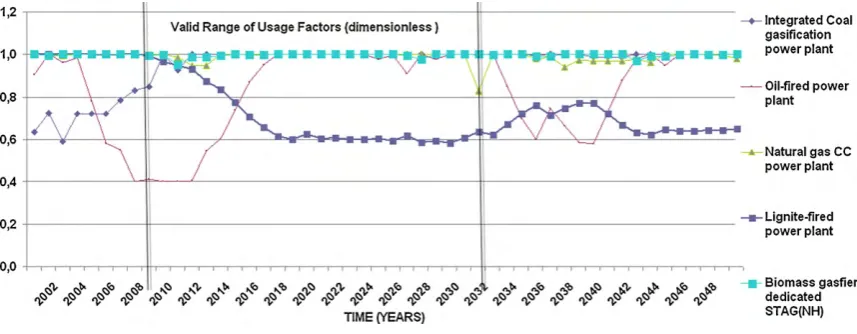
producing technology, in order to extract more accurate results one should modify the inputs by selecting a much wider time period (i.e. till the year 2080), thus being able to investigate the influence of power plants to be built in the distant future. However, adopting an even wider timeframe would lead to two main obstacles: (i) In its current form the computational code examines the 50-year period and its CPU runtime approaches the limits of the acceptable. (ii) A wider time frame would actually cancel the validity of the random-walk forecasting procedure. Since its nature implies a constantly increasing uncertainty of the log-normally distributed results[24], it can be easily understood why the time limits of implementation should be tight (Fig. 6). Therefore, although the code runs for 50 years, only the results concerning the time period 2009–2033 may be considered valid, as was initially planned.
6. Results of the code
The results of the model are presented in the following sub-sections.
6.1. The FPD case
[image:11.595.55.283.58.208.2]The capacity additions appear to have a complex profile as a function of time. In the valid range of results there is no plant category expected to dominate compared to others. Almost all
[image:11.595.83.525.336.530.2]Fig. 6.The investment under increasing uncertainties.
Fig. 7.The calculated capacity orders for FPD.
[image:11.595.82.524.337.729.2]plant types should be ordered to contribute in the increased power demands assumed for the FPD case. The expected yearly capacity orders can be seen inFig. 7.
The expected usage factor smoothly oscillates in high levels for the same reason (Fig. 8).
InFig. 9the cumulative yearly electricity production is shown. It is interesting to note that electricity production succeeds to meet the demand target shown in the upper edge of the curves with a line.
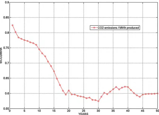
An interesting decrease of CO2emissions per MWhelproduced is expected and this can be seen in the graph of Fig. 10. The anticipated increasing penetration of renewable energy sources – shown inFig. 11– might justify this behaviour. This is also an indication that the optimisation procedure attempted to lower the emission costs thus improving the system’s economy (i.e. compared to the current situation of year 2009).
[image:12.595.48.532.54.200.2]The computational code succeeded to follow the required increase of renewable energy penetration against the conventional
[image:12.595.126.462.230.472.2]Fig. 9.The cumulative energy produced (FPD) in comparison with forecasted demand.
Fig. 10.The expected CO2emissions per produced MWhelfor FPD.
[image:12.595.78.510.608.729.2]power plants. More specifically, starting from the levels of 2001 (close to 8%) the renewables’ contribution rises to the current levels (close to 15% in 2008), and also manages to comply with the EU directives (20,1% in 2010 and 30% in 2020).
The calculated costs breakdown is presented inFig. 12. The expected share of CO2expenses – due to emissions trading – is moderate and slightly rising with time. However its percentage in comparison with the expected fuel costs (almost half) is significant enough to impact the oncoming investment decisions.
The expected financial balance is presented inFig. 13for the entire system. The NPV of the balance curve corresponds to approximately 5109
s
as can be seen inFig. 20.6.2. The ELPD case
[image:13.595.135.472.55.307.2]The ELPD case produced a different decomposition of the Greek electricity sector. Within the range of valid forecasts (years 2009– 2033, Fig. 14) hydroelectric and large onshore wind turbines should dominate the new orders, to maintain the medium levels of electricity demand arising from the constant elasticity hypothesis. Solar PV plants should be installed in the near future whereas the main base-load technology will remain the existing lignite plants. As can be seen inFig. 15the usage factor should vary in lower levels comparing to those observed in the FPD case especially for the lignite fired plants. This happens mainly due to the increasing
Fig. 12.The calculated annual costs and their expected breakdown.
[image:13.595.134.471.483.728.2]costs forecasted for the case of lignite and the large share of lignite power plants at the starting period.
High 90% are optimal levels for usage factors for all but lignite fired plants which should operate at 80% or lower for most of the time. The slight electricity demand increase of ELPD case is shown inFig. 16in comparison with the cumulative electricity produced: an obviously easier target to meet compared to the steep electricity demand increase of the FPD case.
Due to the fact that the required additions are minor, the penetration of renewable energy sources is slower than in the FPD
case. However the expected projection of emissions remains in significantly low levels too. As a result the expected CO2emissions/
MWhel produced are decreasing, as shown in Fig. 17 thus
indicating a consequent economy improvement due to the optimisation algorithm.
The expected expenses and financial balancing breakdowns are shown inFigs. 18 and 19, respectively. The CO2trading costs still contribute significantly to the system costs.
[image:14.595.101.488.52.220.2]It has to be noted that inFigs. 18 and 19, current (nominal) prices are presented meaning that their present value is
[image:14.595.79.508.378.545.2]Fig. 14.The calculated capacity orders for ELPD.
Fig. 15.The calculated usage factor for ELPD.
[image:14.595.61.524.380.703.2]significantly lower, thus resulting to a final NPV close to 7109
s
as shown inFig. 20.
6.3. Sensitivity analysis
Despite of the model’s robustness for most of the input parameters, the system’s aggregate NPV could be severely influenced by the assumption of the interest rates. Therefore, the model’s sensitivity should be further investigated for a wider range of rates assumed. The computational procedure has been
successively performed for acceptable rates in the range 4–8% with increasing step equal to 1%. The resulting sensitivity is shown in Fig. 20for both scenarios.
[image:15.595.135.471.52.294.2]Lower interest rate values lead to higher NPVs as reasonably expected while a more moderate decrease appears for interest rates exceeding 6%. However, negative aggregate NPV is noted for high interest rate values, alerting for deficit systemic operation. It is noted also that the ELPD scenario proves to be less sensitive compared to FPD mainly due to the significantly lower need for future investments and fuel cost.
[image:15.595.133.471.474.728.2]Fig. 17.The expected CO2emissions per produced MWhelfor ELPD.
7. Conclusions
A computational model has been created in order to calculate the optimal power generation capacity additions in the context of future uncertainties. The model incorporates the calculation of the optimal usage factor of the power plant as well as the impact of emissions trading to the finance of the system. The aggregate system NPV constitutes the performance criterion of the study. Focus has been shown on the electricity sector of Greece. Two discrete scenarios have been examined in detail. In the first one, the electricity demand was forecasted directly from historical data (FPD) while in the second, a predetermined elasticity defined the future path of the electricity demand (ELPD).
In the FPD scenario, the anticipated generation mix consists of existing but proven technologies as well as new emerging technologies based on renewable energy sources. The steep increasing of the electricity demand imposes the requirement for power generation originating from all the available technolo-gies, but not uniformly distributed. The low-or-zero fixed and fuel cost of wind generators and hydroelectric plants leads to a significant percentage of the required capacities being based on
these technologies. However, fossil-fueled power plants like lignite and natural gas fired plants, should retain their position as strategic base-load fuels, as is the current situation in Greece. The remaining renewable source technologies like solar PVs and biomass-fired plants are challenged to this race and they may not gain a higher part of power generation unless experience acquired in the future reduces their investment cost. The usage of most plant types should remain in high levels close to 90% in order to meet the demand target. The produced electricity – as calculated by the model –, could comply with the Kyoto protocol requirements, concerning their future penetration against conventional power plants: a share exceeding 20,1% and 30% of the total production for the years 2010 and 2020, respectively should be based on renewable energy sources. Additionally, the stability of the system is ensured due to the restriction of renewable energies far below the limit of 50% of electricity demand.
[image:16.595.125.465.54.304.2]In the ELPD scenario the demand target is moderate and therefore easier to be met by the optimisation algorithm. The low investment and fuel cost of hydroelectric plants favours their future exploitation. Additional plant types based on renewable sources of energy like Solar PVs and biomass-fired plants would be
Fig. 19.The expected system’s financial balancing for ELPD.
[image:16.595.130.463.343.481.2]needed in low percentages, since the demand increase is not steep. For the same reason, the usage factor of future and existing lignite plant types should be moderate and rather lower than those calculated in the FPD scenario.
The model proved to be robust in most of the input parameters but sensitive on the imposed interest rates. Regard-ing the performance of the two investigated scenarios, the ELPD scenario appears to be more efficient in terms of the aggregate anticipated NPV. The moderate requirements for electricity demand (ELPD) allow a higher penetration of renewable energies as a need for compliance with the Kyoto directives. Moreover, their lower fuel and operational costs contribute to a higher performance in terms of system’s economy. On the other hand in the FPD scenario, higher electricity demand levels are expected thus imposing the requirement for intensive use and higher capacity orders from both renewable and conventional plant types. Given the restricted energetic potentials of the renewable sources, the conventional plants should cover higher demand percentages in the expense of the aggregate system’s economic performance, especially due to their higher investment and emission costs. In both case studies a significant improvement with time in the CO2emissions per MWh produced is expected, compared to the currently recorded values, thus indicating an
optimised pattern in CO2 emissions and therefore to the
corresponding emission trading costs.
The results indicated that the model could become a useful tool for energy policy advisors and authorities, state regulators and decision makers. Potential private investors and electricity-related business planners could also benefit from the tool and its results since they may have an overview of the future of different investment options and an indication of the shift in financial attractiveness of the various technologies due to the learning curve effects. As long as they may engage into the energy market arena they could identify their optimal investing options.
Appendix A. Current Greek legal status notes
In Greece the Law 2773/99 constitutes the basic legal background. Two companies, the Regulatory Authority of Energy (RAE) as well as HTSO S.A. (or the so-called ‘‘Hellenic Transmission System Operator’’ or even simpler ‘‘Operator’’) have been created. HTSO is the company that handles the operation of the Hellenic Transmission System of Electric Energy. These two companies are the basic key players of the deregulated electricity market. The main key players of the Greek Electricity market are:
- RAE is an independent authority that manages, suggests and promotes the existence of equal opportunities and fair competi-tion and awards the operacompeti-tion license to producers, providers and all the other players, related to the market.
- HTSO S.A. is a company with a twofold role: The first role is the one being played by P.P.C. in respect to the Transmission System: it ensures the balancing between production and consumption and that the electric energy is provided in a reliable, safe and in terms of quality acceptable way in terms of quality. The second role of HTSO is to settle the market, in other words to act like an energy stock market that arranges on a daily basis who owns to whom. HTSO does not provide electric energy and all the basic exchanging relations that take place are bilateral ones between producers/providers and their customers.
- The Public Power Company (P.P.C.) is one among a number of companies that will be created in the field of electric energy. A stock market pictorial description of the roles could be, P.P.C. is
an admitted company, HTSO is the stock market and RAE is the Capital Market Committee.
Appendix B. The mathematical background for the forecasting tool
Let us consider the following general stochastic differential equation (SDE):
dXt¼Fðt;XtÞdtþGðt;XtÞdWt (1*)
Where:
X is a state vector of process variables (for example, fuel or electricity prices) to simulate.
Wis a Brownian motion vector whose differential oscillates in a range of values generated by normal distribution.
Fis a vector-valued drift-rate function.
Gis a matrix-valued diffusion-rate function.
The drift and diffusion rates, FandG, respectively, are general functions of a real-valued scalar sample timetand state vectorXt. The Eq. (1*) is useful in implementing derived classes that impose additional structure on the drift and diffusion-rate functions. The derived classes of models used in this study are the following.
GBM: The Geometric Brownian Motion Class whose general equation is:
dXt¼
m
ðtÞXtdtþDðt;XtÞVðtÞdWt (2*)Where:
Xtis a state vector of process variables.
m
(t) is the mean drift function derived from the historical data as a mean difference.D(t, Xt) is a diagonal matrix-valued function. Each diagonal
element ofDis the corresponding element of the state vector raised to the corresponding element of an exponent (
a
(t)), which is a vector-valued function:Dðt;XatðtÞÞ.V(t) is a matrix-valued volatility rate function.
dW(t) is a Brownian motion vector (noise) differential which is equal to
e
pffiffiffiffiffidtande
2N(0,1).MR: The Hull-White/Vasicek (HWV) Gaussian Diffusion—Mean Reverting Class:
dXt¼SðtÞ½LðtÞ XtdtþVðtÞdWt (3*)
Where:
Xtis a state vector of process variables.
S(t) is the reverting speed function derived from the historical data.
L(t) is the expected long run mean function.
V(t) is a matrix-valued volatility rate function.
dW(t) is a Brownian motion vector (noise) differential which is equal to
e
pffiffiffiffiffidtande
2N(0,1).References
[1] Rentizelas A, Tziralis G, Kirytopoulos K. Incorporating uncertainty in optimal investment decisions. World Rev Entrepreneurship Manage Sustain Dev 2007;(3/4):273–83.
[3] Rentizelas A, Tolis A, Tatsiopoulos I. Biomass district energy trigeneration systems: emissions reduction and financial impact. Water Air Soil Pollut Focus 2009;9(1–2):139–50.
[4] Huang Y, Wu J. A portfolio risk analysis on electricity supply planning. Energy Policy 2009;37(2):744–61.
[5] Heinrich G, Howells M, Basson L, Petrie J. Electricity supply industry modelling
for multiple objectives under demand growth uncertainty. Energy
2007;32(11):2210–29.
[6] Keppo J, Lu H. Real options and a large producer: the case of electricity markets. Energy Econ 2003;25:459–72.
[7] Laurikka H. Option value of gasification technology within an emissions trading scheme. Energy Policy 2006;34:3916–28.
[8] Laurikka H, Koljonen T. Emissions trading and investment decisions in the power sector—a case study in Finland. Energy Policy 2006;34:1063–74. [9] Niemeyer V. Climate science needs for long-term power sector investment
decisions. EPRI; 2005.
[10] International Energy Agency. Statistics for Greece, 08.12.08,www.iea.org; 2005.
[11] Sood Y, Padhy N, Gupta H, Analysis. Management of wheeling transactions based on AI Techniques under deregulated environment of power sector. Water Energy Int J 2001;58(1):45–52.
[12] Sood Y, Padhy N, Gupta H. Evolutionary programming based algorithm for selection of wheeling options. In: IEEE Power Engineering Society winter meeting; 2001.
[13] Christie D, Wollenberg F, Wangensteen I. Transmission management in the deregulated environment. Proc IEEE 2000;88:70–195.
[14] Svensson E, Berntsson T, Stro¨mberg AB, Patriksson M. An optimisation meth-odology for identifying robust process integration investments under uncer-tainty. Energy Policy 2009;37(2):680–5.
[15] Sahinidis N. Optimisation under uncertainty state of the art and opportunities. Comp Chem Eng 2004;28:971–83.
[16] Kloeden PE, Platen E. Numerical solution of stochastic differential equations. Berlin: Springer; 1999.
[17] Shreve R. Stochastic calculus for finance ii: continuous-time models. Springer-Verlag; 2004.
[18] Box G, Jenkins J, Reinsel G. Time series analysis: forecasting and control, 3rd ed., Upper Saddle River, NJ: Prentice Hall; 1994.
[19] Baillie R, Bollerslev T. Prediction in dynamic models with time-dependent conditional variances. J Econometrics 1992;52:91–113.
[20] McCullough BD, Renfro C. Benchmarks and software standards: a case study of GARCH procedures. J Econ Soc Meas 1998;25:59–71.
[21] Botterud A, Korpas M. A stochastic dynamic model for optimal timing of investments in new generation capacity in restructured power systems. Electr Power Energy Syst 2007;9(2):163–74.
[22] Barlow MT. A diffusion model for electricity prices. Math Financ 2002; 12(4):287–98.
[23] Audet N, Heiskanen P, Keppo J, Vehvilainen I. Modeling electricity forward curve dynamics in the Nordic market. In: Bunn DW, editor. Modeling prices
in competitive electricity markets. New York: Wiley Series in Financ Econ; 2003 .
[24] Dixit A, Pindyck R. Investment under uncertainty. Princeton, NJ: Princeton University Press; 1994.
[25] Glasserman G. Monte Carlo methods in financial engineering. Springer-Verlag; 2004.
[26] Schittkowski K. NLQPL: a FORTRAN-subroutine solving constrained nonlinear programming problems. Ann Oper Res 1985;5:485–500.
[27] Biggs M. In: Dixon LCW, Szergo GP, editors. Constrained minimisation using recursive quadratic programming, towards global optimisation. North-Hol-land; 1975. p. 341–9.
[28] Han S. A globally convergent method for nonlinear programming. J Optim Theory Appl 1977;22:297–331.
[29] Powell M. A fast algorithm for nonlinearly constrained optimisation calcula-tions. Numerical analysis. In: Watson GA, editor. Lecture notes in mathemat-ics, vol. 630. Springer-Verlag; 1978.
[30] Fletcher R. Practical methods of optimisation. John Wiley and Sons; 1987. [31] Gill P, Murray W, Wright M. Practical optimisation. London: Academic Press;
1981.
[32] Powell M. In: Bachem A, Grotschel M, Korte B, editors. Variable metric methods for constrained optimisation. Mathematical programming: the state of the art. Springer-Verlag; 1983. p. 88–311.
[33] Biggs M, Hernandez M. Using the KKT matrix in an augmented Lagrangian SQP method for sparse constrained optimisation. J Optim Theory Appl 1995; 85:201–20.
[34] Powell M. In: Mangasarian OL, Meyer RR, Robinson SM, editors. The
convergence of variable metric methods for nonlinearly constrained optimisation calculations Nonlinear programming, vol. 3. Academic Press; 1978 .
[35] Maribu KM, Fleten SE. Combined heat and power in commercial buildings: investment and risk analysis. Energy J 2008;29:2.
[36] Clewlow L, Strickland C. Energy derivatives: pricing and risk management. London: Lacima Publications; 2000.
[37] HTSO S.A. Hellenic Transmission System Operator, Statistics for the years 2001–2008. 13.12.08,www.desmie.gr; 2008.
[38] Narayan PK, Smyth R. Multivariate granger causality between electricity consumption, exports and GDP: evidence from a panel of Middle Eastern countries. Energy Policy 2009;37(1):229–36.
[39] General Secretariat of Statistical Service of Greece. 09.12.08,http://www. statistics.gr/; 2008.
[40] Point-Carbon. Carbon Market Indicator. 01.12.2008,http://www.pointcarbon. com; 2008.
[41] Natural Gas Company of Attica. Statistics for the years 2001–2008. 13.12.08. http://www.aerioattikis.gr/; 2008.
[42] Tatsiopoulos I, Tolis A. Economic aspects of the cotton-stalk biomass logistics and comparison of supply chain methods. Biomass Bioenergy J 2003;24:199– 214.