Technical Appendix to : Understanding Liquidity and Credit Risks in the Financial Crisis

S

TRATHCLYDE

D

ISCUSSION

P

APERS IN

E

CONOMICS

D

EPARTMENT OF

E

CONOMICS

U

NIVERSITY OF

S

TRATHCLYDE

G

LASGOW

TECHNICAL APPENDIX TO: UNDERSTANDING LIQUIDITY

AND CREDIT RISKS IN THE FINANCIAL CRISIS*

B

Y

DEBORAH

GEFANG,

GARY

KOOP

AND

SIMON

M.

POTTER

Technical Appendix to: Understanding Liquidity

and Credit Risks in the Financial Crisis

Deborah Gefang

Department of Economics University of Lancaster email: d.gefang@lancaster.ac.uk

Gary Koop

Department of Economics University of Strathclyde email: Gary.Koop@strath.ac.uk

Simon M. Potter

Research and Statistics Group Federal Reserve Bank of New York

email: simon.potter@ny.frb.org

October 2010

1

The Gibbs Sampler

This section describes the detailed Gibbs sampler for Bayesian estimation. For all notation, please see the original paper.

1.1 Generating Lkt and Ct

To generateLktand Ct, we …rst transform the dynamic factor model into a

state space form. Let S_ijkt = Sijkt

0

ikXt; and Djt = Djt 0Zt. The measurement

equation of the model can be written as: 0 B B B B B B B B B B B B B B B B B B B B B B B B B B B B B B B B B B B B B B @

D_1t D_2t ::: D_{J t} S_111t S_211t ::: S_I11t S_121t S_221t ::: S_I21t

::: S_IJ1t S_112t S_212t ::: S_IJ2t

::: S_11Kt S_21Kt ::: S_{IJ Kt}

1 C C C C C C C C C C C C C C C C C C C C C C C C C C C C C C C C C C C C C C A = 0 B B B B B B B B B B B B B B B B B B B B B B B B B B B B B B B B B B B B B B B B B B @ C

1 0 0 ::: 0

C

2 0 0 ::: 0

::: ::: :::: C

J 0 0 ::: 0 S

11 S111 0 ::: 0

S

21 S111 0 ::: 0

::: ::: :::: S

I1 SI11 0 ::: 0

S

12 S121 0 ::: 0

S

22 S221 0 ::: 0

::: ::: :::: S

I2 SI21 0 ::: 0

::: ::: :::: S

IJ SIJ1 0 ::: 0

S

11 0 S112 ::: 0

S

21 0 S212 ::: 0

::: ::: :::: S

IJ 0 SIJ2 ::: 0

::: ::: :::: S

11 0 0 ::: S11K

S

21 0 0 ::: S21K

::: ::: :::: S

IJ 0 0 ::: SIJ K 1 C C C C C C C C C C C C C C C C C C C C C C C C C C C C C C C C C C C C C C C C C C A 0 B B @ Ct L1t :: LKt 1 C C A+ 0 B B B B B B B B B B B B B B B B B B B B B B B B B B B B B B B B B B B B B B B B B B @

"D_1t "D_2t ::: "D J t "S 111t "S 211t ::: "S_I11t "S_121t "S_221t ::: "S_I21t

::: "S_IJ1t "S_112t "S_212t ::: "S_IJ2t

::: "S_11Kt "S_21Kt ::: "S_{IJ Kt}

1 C C C C C C C C C C C C C C C C C C C C C C C C C C C C C C C C C C C C C C C C C C A (1 )

(yt=H t+et) (2)

where et i:i:d:N(0; R), the size of yt is J +IJ K by 1, the size of H is

J+IJ K by 1 +K, and the size of _t is 1 +K by 1. The transition equation can be written as

0 B B @

Ct L1t

::: LKt 1 C C A= 0 B B @ C

0(sCt) L

10(sLt) ::: L K0(sLt)

1 C C A+ 0 B B @ C

1(sCt) 0 ::: 0

0 L₁₁(sL_t) ::: 0

:::

0 0 ::: L_K1(sL_t)

1 C C A 0 B B @

Ct 1

L1;t 1

::: LK;t 1

1 C C A+ 0 B B @

C(sCt) Ct

1L(sLt) L1t ::: KL(sLt) LKt

1 C C A

(3 )

( _t= _t+F_{t t 1}+ t) (4)

where t i:i:d:N(0; Qt), the size of t is1 +K by1, the size of t is1 +K

by1, and the size ofFt is1 +K by1 +K.

Let _eyt = (y1; y2; :::; yt)0. Following Kim and Nelson (1999, Ch. 8), we

can draw the latent risk factors in the following two steps.

First run Kalman …lter to calculate _tjt=E( _tjyet)and Ptjt=Cov( tjyet)

fort= 1;2; :::; T :

tjt 1 = t+Ft t 1 P_{tjt 1}=FtPtjt 1F

0

t +Qt

tjt= tjt 1+Ptjt 1H 0

(HPtjt 1H 0

+R) 1(yt H tjt 1)

Ptjt=Ptjt 1 Ptjt 1H 0

(HPtjt 1H 0

Next, we draw _T based on the last iteration of the Kalman …lter:

TjeyT N( TjT; PTjT)

Let _t+1= (Ct+1; L1;t+1; :::; LK;t+1)0. We have

t+1 = t+1+Ft+1 t+ t+1

De…ningQt+1 the variance of t+1, fort=T 1; T 2; :::;1, we can derive

tjeyT backward from

tjyet; t+1 N( tjt; _t+1; Ptjt; t+1)

where

tjt; t+1 = tjt+PtjtF

0

t+1fFt+1PtjtF

0

t+1+Qt+1g 1( t+1 t+1 Ft+1 tjt)

Ptjt; t+1 =Ptjt PtjtF

0

t+1fFt+1PtjtF

0

t+1+Qt+1g 1Ft+1Ptjt

There are many observations missing, especially in the CDS data. To treat the missing elements inyt, following Durbin and Koopman (2008, Ch.

4), we replaceyt,H andR byyt,Ht and Rt, where yt =Wtyt,Ht =WtH

andR_t =WtRW

0

t, withWtbeing the known matrix whose rows are a subset

of rows of the identity matrixIJ+IJ K that correspond to the observed values

in yt. Thus, we adjust the dimensions of H and R to account for the fact

that there is no new information added to the Kalman …lter when data are missing.1

1.2 Draw Parameters for the Measurement Equations

Generating 2

ijkS, Conditional on Sijkt, Sijk, Sij, ik, Lkt and

Ct.

Prior

hijkS G(s_ijkS2 ; ijkS)

where hijkS = ijkS2 . G denotes a Gamma distribution. Details of the

distribution can be found in Koop (2003, p.326).

Posterior

hijkSjSijkt; Sijk; Sij; ik; Lkt; Ct G(s_ijkS2 ; ijkS)

where

ijkS=T TSmijk+ ijkS and

s2_ijkS =

PT

t=1(eSijkt)2+ ijkSs2ijkS ijkS

whereeS_ijkt=Sijkt SijkLkt SijCt

0

ikXt ifSijkt is observed,TSmijk is the number of missing observations inSijk.

Generating S_ijk, Conditional on Sijkt, Sij, ik, hijkS, Lkt and

Ct.

LetS_ijkt[ =Sijkt

0

ikXt SijCtifSijktis observed. We transform each

measurement equation into the following form:

S_ijkt[ = S_ijkLkt+"Sijkt (5)

Prior S

ijk N(b S ijk; V

S

ijk) with

S ijk>0

Posterior S

ijkjSijkt; Sij; ik; hijkS; Lkt; Ct N(b S ijk; V

S

ijk)with

S ijk >0

where

V S ijk =fV

1 S ijk

+hijkSL

0

kLkg 1

and

b S ijk =V

S ijkfV

1 S ijk

b S

ijk +hijkSL 0

kSijk[ g

whereS_ijk[ = [S_ijk[ ₁; S_ijk[ ₂; :::; S_ijkT[ ]0 and Lk= [Lk;1; Lk;2; :::; LkT]

0 .

Generating S_ij, Conditional on Sijkt, Sijk, ik, hijkS, Lkt and

Ct.

LetS_ijkt\ =Sijkt SijkLkt

0

ikXtifSijktis observed. The corresponding

measurement equation can be rewritten as

S_ijkt\ = S_ijCt+"Sijkt (6)

Prior S

ij N(b S

ij; V Sij) with

Posterior S

ijjSijkt; Sijk; ik; hijkS; Lkt; Ct N(b S

ij; V Sij) with

S ij >0

where

V S ij =fV

1 S ij

+ k_X=K

k=1 hijkC

0

C_g 1

and

b S

ij =V SijfV 1 S ij

b S ij+

k_X=K

k=1 hijkC

0

S_ijk\ _g

whereS_ijk\ = [S_ijk\ ₁; S_ijk\ ₂; :::; S_ijkT\ ]0 and C= [C1; C2; :::; CT]

0 .

Generating _ik, Conditional on Sijkt, Sijk, Sij, hijkS, Lkt and

Ct.

LetS_ijkt] =Sijkt SijkLkt SijCtifSijktis observed. The corresponding

measurement equation can be transformed into:

S_ijkt] = 0_ikXt+"Sijkt (7)

Prior

ik N(b ik; V ik)

Posterior

ikjSijkt; Sijk; Sij; hijkS; Lkt; Ct N(b ik; V ik) where

V _ik =_fV 1 ik+

j=J

X

j=1 hijkX

0

X_g 1

and

b _ik =V _ikfV 1 ikb ik +

j=J

X

j=1 hijkX

0

S_ijk] _g

whereS_ijk] = [S_ijk] ₁; S_ijk] ₂; :::; S_ijkT] ]0 and X= [X1; X2; :::; Xt]0.

Prior

hjD G(sjD2; jD) wherehjD = jD2

Posterior

hjDjDjt; Cj ; ; Ct G(sjD2; jD)

where

jD =T TDmjt + jD and

s_jD2 =

PT

t=1(eDjt)2+ jDs2jD jD

where T_Dm

jt is the total number of missing observations inDj, e

D jt =Djt C

j Ct

0

Zt ifDjt is observed.

Generating C_j , Conditional on Djt, , hjD and Ct.

Let D[_jt = Djt 0Zt if Djt is observed. We rewrite the measurement

equation for the credit default variable as:

D[_jt = C_j Ct+"Djt (8)

Prior C

j N(b C

j; V Cj) with

C j >0

Posterior C

j jDjt; hjD; ; Ct N(b C

j; V Cj) with

C j >0

where

V C j =fV

1 C j

+hjDC

0

C_g 1

and

b C

j =V CjfV 1 C j

b C

j +hjDC 0

D[_jg

whereD[_j = [D[_j1; D[_j2; :::; D_jT[ ]0 and C= [C1; C2; :::; CT]0.

Generating , Conditional on Djt, Cj, hjD and Ct.

LetD\_jt =Djt Cj Ct ifDjt is observed. We rewrite the corresponding

measurement equation as:

Prior

N(b ; V )

Posterior

jDjt; hjD; Cj ; Ct N(b ; V ) where

V =_fV 1+ j=J

X

j=1 hjDZ

0

Z_g 1

and

b =V _fV 1b + j=J

X

j=1 hjDZ

0

D\_jg

whereD\_j = [D\_j1; D\_j2:::; D_jT\ ]0 andZ = [Z1; Z2; :::; ZT]

0 .

1.3 Draw Parameters for the Latent Risk Equations

Without loss of generality, we setsL_t = 0 ifsL_t is in ‘good’state for liquidity risk, and sL_t = 1 if sL_t is in ‘bad’ state for liquidity risk. Likewise, we set sC_t = 0 if sC_t is in ‘good’ state for credit risk, and sC_t = 1 if sC_t is in ‘bad’ state for credit risk.

For notation convenience, we rewrite the state equations as follows:

Lkt= Lk00+ Lk01sLt + ( Lk10+ kL11sLt)Lk;t 1+ kL(sLt)vktL (10)

Ct= C00+ C01sCt + ( C10+ C11sCt )Ct 1+ C(sCt )vtC (11)

where

L

k00= Lk0(GL), Lk00+ Lk01= Lk0(BL) L

k10= Lk1(GL), Lk10+ Lk11= Lk1(BL)

and

C

00= C0(GC), 00C + C01= C0(BC) C

10= C1(GC), 10C + C11= C1(BC)

Considering that latent risks are more volatile on average in the bad states, we de…ne

2

kL(BL) = 2kL(GL)(1 +hkLB)

2

C(BC) = 2C(GC)(1 +hCB)

Generating L_k00, L_k01, _kL₁₀, L_k11, Conditional on Lkt and kL(sLt).

Dividing both sides of the state equation by kL(sLt), we have

Ly_kt= L_k00xy_1t+ L_k01xyy_1t+ L_k10xy_2t+ L_k11xyy_2t+vL_kt (12)

where

Ly_kt= Lkt kL(sLt)

xy_1t= 1 kL(sLt)

xyy_1t= s L t

kL(sLt)

xy_2t= Lk;t 1 kL(sLt)

xyy_2t= Lk;t 1s L t

kL(sLt)

In matrix notation, equation (12) can be written as

Ly_k=X_kLy b _kL+VkL VkL N(0; IT) (13)

where

X_kLty = [xy_1t; x₁yy_t; xy_2t; xyy_1t]

and

b _kL = [ L_k00; L_k01; L_k10; L_k11]0

We assume Normal prior for b _kL:

Prior

b _kL N(b

kL; V kL)

with the elements ofb _kL subject to the following restrictions:

L

k102(0;1) Lk10+ Lk112(0;1)

L k00

1 L_k10 < L

k00+ Lk01

1 L_k10 L_k11

Posterior

b _kL N(b _kL; V _kL)R(b _kL)

where

V _kL =_fV 1 kL+ (X

y

kL)

0

X_kLy _g 1 and

b _kL =V _kLfV 1 kLb

1 kL+ (X

y

kL)

0

Ly_kg

Generating 2_kL(GL), Conditional on Lkt, Lk00, Lk01, Lk10, Lk11

and hkLB.

To generate 2_kL(GL), we divide both sides of equation (10) by

p

1 +hkLBsLt

Lz_kt= L_k00xz_1t+ L_k01xzz_1t+ L_k10xz_2t+ L_k11xzz_2t+ kL(GL)vktL (14)

where

Lz_kt= p Lkt

1 +hkLBsLt

xz_1t= p 1

1 +hkLBsLt

xzz_1t= s L t

p

1 +hkLBsLt

xz_2t= _p Lk;t 1 1 +hkLBsLt

xzz_2t= Lk;t 1s L t

p

1 +hkLBsLt

Prior

hkL G(s_kL2; kL)

Posterior

hkL G(s_kL2; kL)

where

kL=T+ kL

and

s2_kL= kLs

2

kL+

Pt=T t=1(Lzkt

L k00xz1t

L k01xzz1t

L k10xz2t

L k11xzz2t)2 kL

GivenhkL, we can derive kL(GL) by kL(GL) = p_h1

GeneratinghkLB, Conditional onLkt, Lk00, Lk01, Lk10, Lk11 and

kL(GL).

To draw hkLB, we divide both sides of equation (10) by kL(GL):

Lx_kt= L_k00x₁x_t+ L_k01xxx_1t+ L_k10xx_2t+ _kL₁₁xxx_2t+vL_kt q

1 +hkLBsLt (15)

where

Lx_kt= Lkt kL(GL)

xx_1t= 1 kL(GL)

xxx_1t = s L t

kL(GL)

xx_2t= Lk;t 1 kL(GL)

xxx_2t = Lk;t 1s L t

kL(GL)

Lethx_kLB = _1+h1

kLB, we set Gamma prior for h

x

kLB: Prior

hx_kLB G(s_kL2_x; _kLx)

subject to the restriction that hx_kLB <1.

Posterior

hx_kLB G(s_kL2_x; _kLx)

subject to the restriction that hx_kLB <1. where

kLx = _kLx+Tx

s2_kLx = kLxs

2

kLx+ PTx

(Lx_kt L_k00xx_1t L_k01xxx_1t L_k10xx_2t L_k11xxx_2t)2 kLx

Note that Tx =_ft: sL_t = 1_g, also hx_kLB depends only on the values of Lx_kt for which sL_t = 1.

Once hx_kLB is drawn from the above posterior, we can calculatehkLB by

hkLB = _hx1 kLB

1.

Dividing both sides of equation (11) by C(sCt ), we have

C_ty= C₀₀z₁y_t+ C₀₁z₁yy_t+ C₁₀z₂y_t+ C₁₁z₂yy_t+vC_t (16) where

C_ty= Ct C(sCt )

z₁y_t= 1 C(sCt )

zyy_1t = s C t

C(sCt)

z₂y_t= Ct 1 C(sCt )

zyy_2t = Ct 1s C t

C(sCt)

In matrix notation, equation (12) can be written as

Cy=Z_Cyb _C+VC VC N(0; IT) (17)

where

Z_Cty = [z₁y_t; z₁yy_t; z₂y_t; zyy_1t]

and

b _C = [ C₀₀; C₀₁; C₁₀; C₁₁]0

We assume Normal prior for b _C:

Prior

b _C N(b

C; V C)

with the elements ofb _C subject to the following restrictions:

C

102(0;1) C10+ C112(0;1)

C

00

1 C₁₀ <

C

00+ C01

1 C₁₀ C₁₁

To save space, we useR(b _C) to denote these additional restrictions.

Posterior

b _C N(b _C; V _C)R(b _C)

where

V _C =_fV 1 C + (Z

y

C)

0

Z_Cy_g 1 and

b _C =V _CfV 1 Cb

1 C+ (Z

y

C)

0

Generating 2_C(GC), Conditional on Ct, C00, C01, C10, C11 and hCB.

To generate 2_C(GC), we divide both sides of equation (11) by

p

1 +hCBsCt

C_tz= C₀₀z₁z_t+ C₀₁z₁zz_t+ C₁₀z₂z_t+ C₁₁zzz_2t+ C(GC)vtC (18)

where

C_tz= p Ct

1 +hCBsCt

z₁z_t= p 1

1 +hCBsCt

z₁zz_t = s C t

p

1 +hCBsCt

z₂z_t= p Ct 1

1 +hCBsCt

z₂zz_t = Ct 1s C t

p

1 +hCBsCt

Prior

hC G(sC2; C)where hC = C2(GC) Posterior

hC G(s_C2; C)

where

C =T+ C

and

s2_C = Cs

2

C+

Pt=T

t=1(Ctz C00z1zt C01z1zzt C10zz2t C11z2zzt)2 C

GivenhC, we can derive C(GC) by C(GC) = p1_h

C.

Generating hCB, Conditional on Ct, C00, C01, C10, C11 and

To draw hCB, we divide both sides of equation (11) by C(GC):

C_tx= C₀₀z₁x_t+ C₀₁z₁xx_t+ C₁₀z₂x_t+ ₁₁Cz₂xx_t+v_tC q

1 +hCBsCt (19)

where

C_tx= Ct C(GC)

zx_1t= 1 C(GC)

z₁xx_t = s C t

C(GC)

zx_2t= Ct 1 C(GC)

z₂xx_t = Ct 1s C t

C(GC)

Lethx_CB = _1+h1

CB, we set Gamma prior forh

x

CB: Prior

hx_CB G(s_C2_x; _Cx)

subject to the restriction that hx_CB <1.

Posterior

hx_CB G(s_C2_x; _Cx)

subject to the restriction that hx_CB <1. where

Cx = Cx+T_Cx

s2_Cx =

Cxs2_Cx+

PT_Cx_(Cx

t C00z1xt C

01z1xxt C

10z2xt C

11z2xxt)2 Cx

Note thatT_Cx =_ft:sC

t = 1g, andhxCB depends only on the values of Ctx for

which sC_t = 1.

Once hx_CB is drawn from the above posterior,hCB can be calculated by

hCB = _hx1 CB

1.4 Generating sL

t, sCt and M

Generate sL_t and sC_t , Conditional on M, Lkt, Ct and the other

model parameters

We use the multimove Gibbs-sampling method described in Kim and Nelson (1999, Ch 9) to draw the latent Markov-Switching states.

To summarize, we …rst run Hamilton’s (1989) …lter to get the probability f(stjLekt;Cet)fort= 1;2; :::; T and save them, whereLekt= [Lk1; Lk2; :::; Lkt]

0

and Cet = [C1; C2; :::; Ct]0. Then we generate sT from the last iteration of

the …lter. After that, we recursively generate st conditional on Lekt, Cet and

st+1 fort=T 1; T 2; :::1.

Generate M, Conditional on sL

t, sCt , Lkt, Ct and the other

model parameters

As explained in Chib (1996), given _esT, the posterior distribution of the

transition matrix M can be derived without regard to the sampling model. Let vector mb be the bth column of M. We elicit a Dirichlet prior for

mb:

mb D( 1;b; 2;b; :::; a;b)

Thus, the posterior formb is:

mbjesT D( 1;b+q1;b; 2;b+q2;b; :::; a;b+qa;b)

whereqa;b is the number of transitions fromst=btost+1=ain the vector e

sT.

2

Priors and Prior Sensitivity Analysis

2.1 Elicited Priors

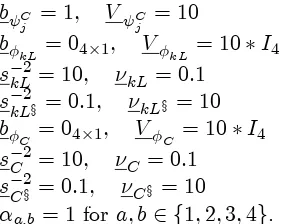
The results presented in the paper involve the following priors: s_ijkS2 = 10; _ijkS = 0:1

b S

ijk = 1; V Sijk = 10 b S

ij = 1; V Sij = 10 b = 0; V = 10

b

b C

j = 1; V Cj = 10 b

kL= 04 1; V kL= 10 I4 s_kL2= 10; _kL= 0:1

s_kL2_x = 0:1; _kLx = 10

b

C = 04 1; V C = 10 I4 s_C2= 10; _C = 0:1

s_C2_x = 0:1; _Cx = 10

a;b= 1 fora; b2 f1;2;3;4g.

2.2 Prior Sensitivity Analysis

The following priors are used for prior sensitivity analysis. s_ijkS2 = 1; _ijkS = 1

b S

ijk = 0; V S

ijk = 100

b S

ij = 0; V Sij = 100

b = 0; V = 100

b

ik = 0; V ik = 100

s_jD2 = 1; _jD = 1

b C

j = 1; V Cj = 100

b

kL= 04 1; V kL= 4 I4 s_kL2= 1; _kL= 1

s_kL2_x = 0:1; _kLx = 10

b

C = 04 1; V C = 4 I4 s_C2= 1; _C = 1

s_C2_x = 0:1; _Cx = 10

a;b= 2 fora; b2 f1;2;3;4g.

Empirical results using these new priors are as follows.

Table 2: Posterior Mean of Transition Probabilities (Posterior standard deviations in parentheses)

(GL; GC) (BL; GC) (GL; BC) (BL; BC)

(GL; GC)

0:972 (0:007)

0:231 (0:127)

0:246 (0:132)

0:221 (0:096)

(BL; GC)

0:009 (0:005)

0:258 (0:140)

0:235 (0:132)

0:198 (0:111)

(GL; BC) 0:009

(0:005)

0:187 (0:113)

0:251 (0:128)

0:149 (0:087)

(BL; BC)

0:010 (0:005)

0:324 (0:150)

0:267 (0:142)

Table 3: Proportion of Variance of Spreads Attributable to Each Component (USD) var(L) var ( C) var(X) cov(L,C) cov(L,X) cov(C,X) var(e) barclays1m 0.8918 0.0000 0.0008 0.0000 0.0020 0.0000 0.1054

barclays3m 0.8208 0.0720 0.0000 0.0966 -0.0002 0.0000 0.0108

barclays12m 0.2720 0.4217 0.0000 0.1345 0.0000 0.0000 0.1718

btmuf j1m 0.8755 0.0042 0.0011 0.0239 0.0023 0.0000 0.0930

btmuf j3m 0.7801 0.1027 0.0000 0.1125 -0.0003 0.0000 0.0050

btmuf j12m 0.2129 0.5345 0.0000 0.1340 0.0000 0.0000 0.1186

citibank1m 0.8963 0.0015 0.0013 0.0146 0.0025 0.0000 0.0836

citibank3m 0.7715 0.1101 0.0000 0.1158 -0.0003 0.0000 0.0029

citibank12m 0.1991 0.5585 0.0000 0.1325 0.0000 0.0000 0.1099

deutschebank1m 0.9094 0.0000 0.0014 0.0002 0.0026 0.0000 0.0864

deutschebank3m 0.7876 0.0982 0.0000 0.1106 -0.0003 0.0000 0.0039

deutschebank12m 0.2908 0.4672 0.0000 0.1465 0.0000 0.0000 0.0956

hbos1m 0.8682 0.0000 0.0009 0.0001 0.0020 0.0000 0.1287

hbos3m 0.8352 0.0038 0.0000 0.0221 -0.0002 0.0000 0.1391

hbos12m 0.6070 0.0496 0.0000 0.0688 0.0000 0.0000 0.2747

hsbc1m 0.9085 0.0001 0.0013 0.0028 0.0025 0.0000 0.0848

hsbc3m 0.7876 0.0992 0.0000 0.1111 -0.0003 0.0000 0.0024

hsbc12m 0.2660 0.4843 0.0000 0.1426 0.0000 0.0000 0.1070

jpmc1m 0.9009 0.0000 0.0015 0.0003 0.0027 0.0000 0.0946

jpmc3m 0.7692 0.1076 0.0000 0.1144 -0.0003 0.0000 0.0091

jpmc12m 0.1849 0.5484 0.0000 0.1265 0.0000 0.0000 0.1403

lloyds1m 0.9186 0.0000 0.0013 0.0005 0.0026 0.0000 0.0770

lloyds3m 0.7716 0.1103 0.0000 0.1160 -0.0003 0.0000 0.0024

lloyds12m 0.1903 0.5624 0.0000 0.1300 0.0000 0.0000 0.1173

rabobank1m 0.8999 0.0006 0.0015 0.0089 0.0027 0.0000 0.0864

rabobank3m 0.7460 0.1237 0.0000 0.1208 -0.0003 0.0000 0.0098

rabobank12m 0.2110 0.5224 0.0000 0.1319 0.0000 0.0000 0.1346

rboscotland1m 0.9163 0.0001 0.0012 0.0036 0.0024 0.0000 0.0764

rboscotland3m 0.7686 0.1099 0.0000 0.1155 -0.0003 0.0000 0.0062

rboscotland12m 0.1867 0.5159 0.0000 0.1233 0.0000 0.0000 0.1741

ubs1m 0.9148 0.0001 0.0012 0.0045 0.0024 0.0000 0.0769

ubs3m 0.7560 0.1217 0.0000 0.1206 -0.0003 0.0000 0.0021

ubs12m 0.1929 0.5353 0.0000 0.1276 0.0000 0.0000 0.1441

westlb1m 0.8708 0.0015 0.0013 0.0145 0.0024 0.0000 0.1095

westlb3m 0.7369 0.1307 0.0000 0.1234 -0.0003 0.0000 0.0093

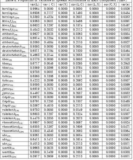
Table 4: Proportion of Variance of Spreads Attributable to Each Component (GBP) var(L) var ( C) var(X) cov(L,C) cov(L,X) cov(C,X) var(e) barclays1m 0.9964 0.0000 0.0000 0.0000 0.0000 0.0000 0.0036

barclays3m 0.6936 0.1117 0.0000 0.1493 0.0000 0.0000 0.0454

barclays12m 0.3393 0.4224 0.0000 0.2031 0.0000 0.0000 0.0352

btmuf j1m 0.9363 0.0081 0.0000 0.0466 0.0000 0.0000 0.0091

btmuf j3m 0.6632 0.1297 0.0000 0.1574 0.0000 0.0000 0.0497

btmuf j12m 0.4042 0.3832 0.0000 0.2112 0.0000 0.0000 0.0013

citibank1m 0.9627 0.0025 0.0000 0.0263 0.0000 0.0000 0.0084

citibank3m 0.6614 0.1204 0.0000 0.1515 0.0000 0.0000 0.0668

citibank12m 0.3860 0.4004 0.0000 0.2110 0.0000 0.0000 0.0027

deutschebank1m 0.9893 0.0000 0.0000 0.0004 0.0000 0.0000 0.0103

deutschebank3m 0.6811 0.1194 0.0000 0.1530 0.0000 0.0000 0.0464

deutschebank12m 0.4663 0.3144 0.0000 0.2055 0.0000 0.0000 0.0138

hbos1m 0.8170 0.0000 0.0000 0.0003 0.0000 0.0000 0.1828

hbos3m 0.6717 0.0046 0.0000 0.0295 0.0000 0.0000 0.2943

hbos12m 0.5569 0.0366 0.0000 0.0764 0.0000 0.0000 0.3301

hsbc1m 0.9705 0.0001 0.0000 0.0057 0.0000 0.0000 0.0236

hsbc3m 0.6560 0.1306 0.0000 0.1571 0.0000 0.0000 0.0563

hsbc12m 0.4222 0.3599 0.0000 0.2092 0.0000 0.0000 0.0087

jpmc1m 0.9895 0.0000 0.0000 0.0005 0.0000 0.0000 0.0099

jpmc3m 0.6919 0.1078 0.0000 0.1465 0.0000 0.0000 0.0538

jpmc12m 0.4497 0.3364 0.0000 0.2087 0.0000 0.0000 0.0052

lloyds1m 0.9978 0.0000 0.0000 0.0009 0.0000 0.0000 0.0012

lloyds3m 0.6791 0.1208 0.0000 0.1537 0.0000 0.0000 0.0465

lloyds12m 0.3867 0.4010 0.0000 0.2113 0.0000 0.0000 0.0010

rabobank1m 0.9702 0.0008 0.0000 0.0149 0.0000 0.0000 0.0141

rabobank3m 0.6683 0.1207 0.0000 0.1524 0.0000 0.0000 0.0587

rabobank12m 0.4470 0.3355 0.0000 0.2078 0.0000 0.0000 0.0097

rboscotland1m 0.9907 0.0002 0.0000 0.0067 0.0000 0.0000 0.0024

rboscotland3m 0.6555 0.1367 0.0000 0.1606 0.0000 0.0000 0.0471

rboscotland12m 0.3503 0.4340 0.0000 0.2093 0.0000 0.0000 0.0064

ubs1m 0.9861 0.0003 0.0000 0.0084 0.0000 0.0000 0.0052

ubs3m 0.6411 0.1411 0.0000 0.1614 0.0000 0.0000 0.0564

ubs12m 0.4013 0.3863 0.0000 0.2113 0.0000 0.0000 0.0011

westlb1m 0.9665 0.0025 0.0000 0.0265 0.0000 0.0000 0.0045

westlb3m 0.6500 0.1459 0.0000 0.1653 0.0000 0.0000 0.0388

Table 5: Proportion of Variance of Spreads Attributable to Each Component (EUR) var(L) var ( C) var(X) cov(L,C) cov(L,X) cov(C,X) var(e) barclays1m 0.8953 0.0000 0.0000 0.0000 0.0000 0.0000 0.1047

barclays3m 0.6521 0.1986 0.0000 0.1391 0.0000 0.0000 0.0101

barclays12m 0.2183 0.5940 0.0000 0.1392 0.0000 0.0000 0.0485

btmuf j1m 0.8509 0.0154 0.0000 0.0441 0.0000 0.0000 0.0896

btmuf j3m 0.6115 0.2391 0.0000 0.1478 0.0000 0.0000 0.0015

btmuf j12m 0.2308 0.5804 0.0000 0.1415 0.0000 0.0000 0.0474

citibank1m 0.8573 0.0045 0.0000 0.0240 0.0000 0.0000 0.1142

citibank3m 0.6327 0.2208 0.0000 0.1445 0.0000 0.0000 0.0020

citibank12m 0.2288 0.5784 0.0000 0.1406 0.0000 0.0000 0.0522

deutschebank1m 0.8600 0.0000 0.0000 0.0004 0.0000 0.0000 0.1396

deutschebank3m 0.5914 0.2377 0.0000 0.1449 0.0000 0.0000 0.0260

deutschebank12m 0.2786 0.5370 0.0000 0.1495 0.0000 0.0000 0.0348

hbos1m 0.8276 0.0000 0.0000 0.0003 0.0000 0.0000 0.1721

hbos3m 0.7510 0.0077 0.0000 0.0290 0.0000 0.0000 0.2123

hbos12m 0.5575 0.0610 0.0000 0.0711 0.0000 0.0000 0.3104

hsbc1m 0.8616 0.0003 0.0000 0.0051 0.0000 0.0000 0.1330

hsbc3m 0.6458 0.2079 0.0000 0.1416 0.0000 0.0000 0.0047

hsbc12m 0.2908 0.5170 0.0000 0.1499 0.0000 0.0000 0.0423

jpmc1m 0.9018 0.0000 0.0000 0.0005 0.0000 0.0000 0.0977

jpmc3m 0.6562 0.2013 0.0000 0.1405 0.0000 0.0000 0.0020

jpmc12m 0.2787 0.5280 0.0000 0.1483 0.0000 0.0000 0.0450

lloyds1m 0.8918 0.0000 0.0000 0.0009 0.0000 0.0000 0.1073

lloyds3m 0.6309 0.2220 0.0000 0.1447 0.0000 0.0000 0.0024

lloyds12m 0.2037 0.6015 0.0000 0.1353 0.0000 0.0000 0.0595

rabobank1m 0.8816 0.0015 0.0000 0.0137 0.0000 0.0000 0.1032

rabobank3m 0.6043 0.2301 0.0000 0.1442 0.0000 0.0000 0.0214

rabobank12m 0.2736 0.5323 0.0000 0.1475 0.0000 0.0000 0.0467

rboscotland1m 0.8773 0.0003 0.0000 0.0060 0.0000 0.0000 0.1164

rboscotland3m 0.6107 0.2350 0.0000 0.1465 0.0000 0.0000 0.0078

rboscotland12m 0.1847 0.6213 0.0000 0.1309 0.0000 0.0000 0.0630

ubs1m 0.8353 0.0005 0.0000 0.0078 0.0000 0.0000 0.1564

ubs3m 0.5832 0.2578 0.0000 0.1499 0.0000 0.0000 0.0091

ubs12m 0.2277 0.5860 0.0000 0.1412 0.0000 0.0000 0.0451

westlb1m 0.8539 0.0043 0.0000 0.0234 0.0000 0.0000 0.1184

westlb3m 0.5929 0.2518 0.0000 0.1494 0.0000 0.0000 0.0059

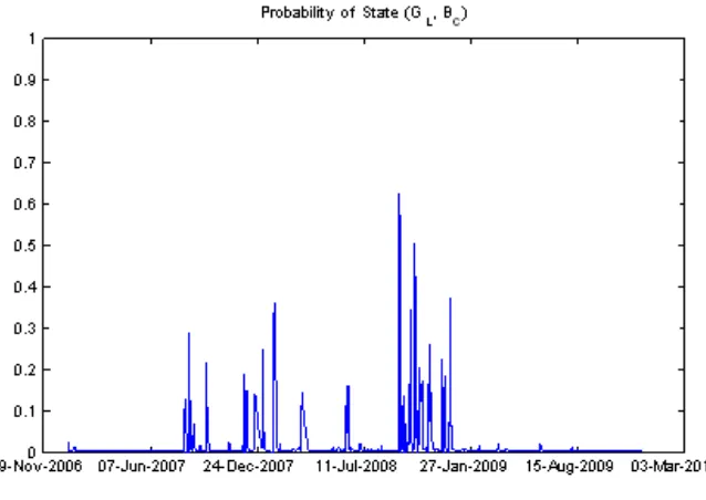
Figure 6

3

Empirical Results Involving Only Eight Banks

Empirical results reported in this section using data of the eight banks for which we do not have any missing observations.

Table 7: Posterior Mean of Transition Probabilities (Posterior standard deviations in parentheses)

(GL; GC) (BL; GC) (GL; BC) (BL; BC)

(GL; GC)

0:950 (0:013)

0:311 (0:134)

0:179 (0:093)

0:047 (0:038)

(BL; GC)

0:019 (0:009)

0:375 (0:149)

0:061 (0:054)

0:069 (0:062)

(GL; BC) 0:018

(0:010)

0:109 (0:096)

0:658 (0:108)

0:107 (0:050)

(BL; BC)

0:013 (0:008)

0:205 (0:141)

0:101 (0:063)

0:777 (0:077)

Table 8: Proportion of Variance of Spreads Attributable to Each Component (USD) var(L) var ( C) var(X) cov(L,C) cov(L,X) cov(C,X) var(e) barclays1m 0.8977 0.0000 0.0008 0.0000 0.0019 0.0000 0.0996

barclays3m 0.7277 0.1088 0.0000 0.1521 -0.0002 0.0000 0.0117

barclays12m 0.1120 0.6091 0.0000 0.1409 0.0000 0.0000 0.1380

citibank1m 0.9021 0.0011 0.0013 0.0172 0.0024 0.0000 0.0758

citibank3m 0.6746 0.1506 0.0000 0.1723 -0.0002 0.0000 0.0027

citibank12m 0.0620 0.7329 0.0000 0.1150 0.0000 0.0000 0.0901

deutschebank1m 0.9155 0.0000 0.0014 0.0004 0.0025 0.0000 0.0803

deutschebank3m 0.7000 0.1319 0.0000 0.1642 -0.0002 0.0000 0.0041

deutschebank12m 0.1412 0.6161 0.0000 0.1593 0.0000 0.0000 0.0835

jpmc1m 0.9095 0.0000 0.0015 0.0006 0.0026 0.0000 0.0859

jpmc3m 0.7100 0.1232 0.0000 0.1598 -0.0002 0.0000 0.0073

jpmc12m 0.0572 0.7153 0.0000 0.1091 0.0000 0.0000 0.1183

lloyds1m 0.9199 0.0001 0.0013 0.0038 0.0025 0.0000 0.0724

lloyds3m 0.6662 0.1572 0.0000 0.1749 -0.0002 0.0000 0.0020

lloyds12m 0.0581 0.7330 0.0000 0.1114 0.0000 0.0000 0.0975

rabobank1m 0.9022 0.0006 0.0015 0.0120 0.0026 0.0000 0.0810

rabobank3m 0.6442 0.1685 0.0000 0.1781 -0.0002 0.0000 0.0094

rabobank12m 0.0740 0.6867 0.0000 0.1216 0.0000 0.0000 0.1177

rboscotland1m 0.9102 0.0006 0.0012 0.0122 0.0023 0.0000 0.0735

rboscotland3m 0.6388 0.1751 0.0000 0.1808 -0.0002 0.0000 0.0055

rboscotland12m 0.0592 0.6820 0.0000 0.1083 0.0000 0.0000 0.1505

ubs1m 0.9131 0.0004 0.0012 0.0108 0.0023 0.0000 0.0721

ubs3m 0.6595 0.1621 0.0000 0.1767 -0.0002 0.0000 0.0019

Table 9: Proportion of Variance of Spreads Attributable to Each Component (GBP) var(L) var ( C) var(X) cov(L,C) cov(L,X) cov(C,X) var(e) barclays1m 0.9964 0.0000 0.0000 0.0000 0.0000 0.0000 0.0036

barclays3m 0.5686 0.1710 0.0000 0.2161 0.0000 0.0000 0.0442

barclays12m 0.1462 0.6117 0.0000 0.2071 0.0000 0.0000 0.0349

citibank1m 0.9605 0.0019 0.0000 0.0292 0.0000 0.0000 0.0084

citibank3m 0.5556 0.1660 0.0000 0.2105 0.0000 0.0000 0.0679

citibank12m 0.2036 0.5581 0.0000 0.2337 0.0000 0.0000 0.0046

deutschebank1m 0.9894 0.0000 0.0000 0.0006 0.0000 0.0000 0.0100

deutschebank3m 0.5797 0.1621 0.0000 0.2124 0.0000 0.0000 0.0458

deutschebank12m 0.3039 0.4289 0.0000 0.2503 0.0000 0.0000 0.0169

jpmc1m 0.9899 0.0000 0.0000 0.0009 0.0000 0.0000 0.0092

jpmc3m 0.6276 0.1232 0.0000 0.1928 0.0000 0.0000 0.0564

jpmc12m 0.2736 0.4696 0.0000 0.2484 0.0000 0.0000 0.0084

lloyds1m 0.9924 0.0001 0.0000 0.0064 0.0000 0.0000 0.0011

lloyds3m 0.5633 0.1735 0.0000 0.2167 0.0000 0.0000 0.0464

lloyds12m 0.2064 0.5553 0.0000 0.2346 0.0000 0.0000 0.0037

rabobank1m 0.9661 0.0008 0.0000 0.0191 0.0000 0.0000 0.0140

rabobank3m 0.5645 0.1652 0.0000 0.2117 0.0000 0.0000 0.0586

rabobank12m 0.2704 0.4706 0.0000 0.2473 0.0000 0.0000 0.0117

rboscotland1m 0.9746 0.0010 0.0000 0.0219 0.0000 0.0000 0.0024

rboscotland3m 0.5044 0.2201 0.0000 0.2309 0.0000 0.0000 0.0446

rboscotland12m 0.1706 0.5986 0.0000 0.2215 0.0000 0.0000 0.0093

ubs1m 0.9749 0.0008 0.0000 0.0191 0.0000 0.0000 0.0052

ubs3m 0.5332 0.1896 0.0000 0.2204 0.0000 0.0000 0.0568

Table 10: Proportion of Variance of Spreads Attributable to Each Component (EUR) var(L) var ( C) var(X) cov(L,C) cov(L,X) cov(C,X) var(e) barclays1m 0.9792 0.0000 0.0000 0.0000 0.0000 0.0000 0.0208

barclays3m 0.4124 0.2921 0.0000 0.2244 0.0000 0.0000 0.0711

barclays12m 0.0401 0.7761 0.0000 0.1137 0.0000 0.0000 0.0701

citibank1m 0.9506 0.0033 0.0000 0.0362 0.0000 0.0000 0.0099

citibank3m 0.4276 0.2956 0.0000 0.2299 0.0000 0.0000 0.0468

citibank12m 0.0587 0.7392 0.0000 0.1346 0.0000 0.0000 0.0675

deutschebank1m 0.9394 0.0000 0.0000 0.0008 0.0000 0.0000 0.0598

deutschebank3m 0.3835 0.3139 0.0000 0.2243 0.0000 0.0000 0.0783

deutschebank12m 0.1060 0.6813 0.0000 0.1737 0.0000 0.0000 0.0391

jpmc1m 0.9963 0.0000 0.0000 0.0012 0.0000 0.0000 0.0025

jpmc3m 0.4955 0.2289 0.0000 0.2177 0.0000 0.0000 0.0579

jpmc12m 0.0945 0.6812 0.0000 0.1639 0.0000 0.0000 0.0604

lloyds1m 0.9866 0.0002 0.0000 0.0081 0.0000 0.0000 0.0051

lloyds3m 0.4056 0.3084 0.0000 0.2287 0.0000 0.0000 0.0573

lloyds12m 0.0439 0.7628 0.0000 0.1180 0.0000 0.0000 0.0753

rabobank1m 0.9554 0.0014 0.0000 0.0237 0.0000 0.0000 0.0194

rabobank3m 0.3925 0.3066 0.0000 0.2243 0.0000 0.0000 0.0767

rabobank12m 0.0895 0.6890 0.0000 0.1604 0.0000 0.0000 0.0611

rboscotland1m 0.9639 0.0018 0.0000 0.0269 0.0000 0.0000 0.0074

rboscotland3m 0.3519 0.3569 0.0000 0.2291 0.0000 0.0000 0.0620

rboscotland12m 0.0340 0.7848 0.0000 0.1053 0.0000 0.0000 0.0758

ubs1m 0.9394 0.0015 0.0000 0.0244 0.0000 0.0000 0.0346

ubs3m 0.3877 0.3353 0.0000 0.2331 0.0000 0.0000 0.0438

Figure 12

4

Empirical Results Involving Di¤erent

Identi…ca-tion AssumpIdenti…ca-tions

In this section, we present the empirical results where we restrict the factor loading for the termi= 2 to unity. Variance decomposition results for EUR show a pattern that di¤ers from that of USD and GBP, which might be caused by the non-negligible correlation betweenL for EUR andC.

Table 12: Posterior Mean of Transition Probabilities (Posterior standard deviations in parentheses)

(GL; GC) (BL; GC) (GL; BC) (BL; BC)

(GL; GC)

0:948 (0:012)

0:257 (0:165)

0:225 (0:127)

0:086 (0:039)

(BL; GC)

0:010 (0:007)

0:273 (0:157)

0:059 (0:064)

0:028 (0:025)

(GL; BC) 0:015

(0:010)

0:157 (0:140)

0:283 (0:144)

0:094 (0:049)

(BL; BC)

0:027 (0:012)

0:312 (0:195)

0:432 (0:150)

Table 13: Proportion of Variance of Spreads Attributable to Each Component (USD) var(L) var ( C) var(X) cov(L,C) cov(L,X) cov(C,X) var(e) barclays1m 0.8649 0.1428 0.0000 -0.0449 0.0000 0.0000 0.0373

barclays3m 0.6123 0.4063 0.0008 -0.0636 -0.0019 -0.0007 0.0470

barclays12m 0.1026 0.9225 0.0000 -0.0393 0.0000 0.0000 0.0142

btmuf j1m 0.8287 0.2160 0.0000 -0.0540 0.0000 0.0000 0.0094

btmuf j3m 0.5612 0.4765 0.0009 -0.0660 -0.0020 -0.0008 0.0302

btmuf j12m 0.1157 0.9216 0.0000 -0.0417 0.0000 0.0000 0.0044

citibank1m 0.8590 0.1899 0.0000 -0.0516 0.0000 0.0000 0.0028

citibank3m 0.4396 0.0000 0.0011 0.0000 -0.0020 0.0000 0.5613

citibank12m 0.1135 0.9235 0.0000 -0.0413 0.0000 0.0000 0.0043

deutschebank1m 0.8673 0.1761 0.0000 -0.0499 0.0000 0.0000 0.0066

deutschebank3m 0.5621 0.4564 0.0009 -0.0646 -0.0020 -0.0008 0.0482

deutschebank12m 0.1462 0.8921 0.0000 -0.0461 0.0000 0.0000 0.0079

hbos1m 0.8996 0.1120 0.0000 -0.0405 0.0000 0.0000 0.0289

hbos3m 0.7227 0.2078 0.0007 -0.0494 -0.0020 -0.0005 0.1207

hbos12m 0.4815 0.3007 0.0000 -0.0485 0.0000 0.0000 0.2663

hsbc1m 0.8724 0.1748 0.0000 -0.0499 0.0000 0.0000 0.0027

hsbc3m 0.5461 0.4757 0.0010 -0.0650 -0.0021 -0.0009 0.0452

hsbc12m 0.1311 0.9090 0.0000 -0.0441 0.0000 0.0000 0.0040

jpmc1m 0.8877 0.1540 0.0000 -0.0472 0.0000 0.0000 0.0056

jpmc3m 0.5126 0.4980 0.0010 -0.0645 -0.0021 -0.0009 0.0558

jpmc12m 0.0927 0.9356 0.0000 -0.0376 0.0000 0.0000 0.0094

lloyds1m 0.8598 0.1902 0.0000 -0.0516 0.0000 0.0000 0.0016

lloyds3m 0.5172 0.5038 0.0010 -0.0651 -0.0020 -0.0009 0.0460

lloyds12m 0.1100 0.9256 0.0000 -0.0408 0.0000 0.0000 0.0051

rabobank1m 0.8415 0.1997 0.0000 -0.0523 0.0000 0.0000 0.0111

rabobank3m 0.4892 0.5206 0.0010 -0.0644 -0.0020 -0.0009 0.0565

rabobank12m 0.1051 0.9238 0.0000 -0.0398 0.0000 0.0000 0.0109

rboscotland1m 0.8413 0.1979 0.0000 -0.0521 0.0000 0.0000 0.0129

rboscotland3m 0.5271 0.4993 0.0009 -0.0654 -0.0019 -0.0008 0.0410

rboscotland12m 0.0880 0.9349 0.0000 -0.0366 0.0000 0.0000 0.0137

ubs1m 0.8592 0.1911 0.0000 -0.0517 0.0000 0.0000 0.0014

ubs3m 0.5241 0.5035 0.0009 -0.0656 -0.0020 -0.0008 0.0398

ubs12m 0.0992 0.9304 0.0000 -0.0388 0.0000 0.0000 0.0091

westlb1m 0.8273 0.2133 0.0000 -0.0536 0.0000 0.0000 0.0131

westlb3m 0.5125 0.5246 0.0009 -0.0662 -0.0019 -0.0009 0.0310

Table 14: Proportion of Variance of Spreads Attributable to Each Component (GBP) var(L) var ( C) var(X) cov(L,C) cov(L,X) cov(C,X) var(e) barclays1m 0.6467 0.3521 0.0000 -0.0024 0.0000 0.0000 0.0036

barclays3m 0.3563 0.6093 0.0000 -0.0023 0.0000 0.0000 0.0367

barclays12m 0.1239 0.8419 0.0000 -0.0016 0.0000 0.0000 0.0358

btmuf j1m 0.5813 0.4139 0.0000 -0.0024 0.0000 0.0000 0.0073

btmuf j3m 0.3382 0.6222 0.0000 -0.0023 0.0000 0.0000 0.0419

btmuf j12m 0.2363 0.7215 0.0000 -0.0021 0.0000 0.0000 0.0442

citibank1m 0.6523 0.3411 0.0000 -0.0024 0.0000 0.0000 0.0090

citibank3m 0.3353 0.0000 0.0000 0.0000 0.0000 0.0000 0.6647

citibank12m 0.2295 0.7222 0.0000 -0.0020 0.0000 0.0000 0.0503

deutschebank1m 0.7115 0.2830 0.0000 -0.0022 0.0000 0.0000 0.0077

deutschebank3m 0.4049 0.5467 0.0000 -0.0023 0.0000 0.0000 0.0508

deutschebank12m 0.2835 0.6578 0.0000 -0.0022 0.0000 0.0000 0.0609

hbos1m 0.6838 0.1970 0.0000 -0.0018 0.0000 0.0000 0.1211

hbos3m 0.5251 0.2344 0.0000 -0.0018 0.0000 0.0000 0.2422

hbos12m 0.4683 0.2377 0.0000 -0.0017 0.0000 0.0000 0.2956

hsbc1m 0.6205 0.3569 0.0000 -0.0024 0.0000 0.0000 0.0249

hsbc3m 0.3494 0.5983 0.0000 -0.0023 0.0000 0.0000 0.0545

hsbc12m 0.2348 0.7103 0.0000 -0.0020 0.0000 0.0000 0.0569

jpmc1m 0.7423 0.2568 0.0000 -0.0022 0.0000 0.0000 0.0031

jpmc3m 0.3885 0.5590 0.0000 -0.0023 0.0000 0.0000 0.0548

jpmc12m 0.2803 0.6619 0.0000 -0.0021 0.0000 0.0000 0.0599

lloyds1m 0.6755 0.3258 0.0000 -0.0023 0.0000 0.0000 0.0010

lloyds3m 0.3529 0.6085 0.0000 -0.0023 0.0000 0.0000 0.0409

lloyds12m 0.2328 0.7231 0.0000 -0.0020 0.0000 0.0000 0.0461

rabobank1m 0.6685 0.3194 0.0000 -0.0023 0.0000 0.0000 0.0144

rabobank3m 0.3734 0.5736 0.0000 -0.0023 0.0000 0.0000 0.0553

rabobank12m 0.2675 0.6775 0.0000 -0.0021 0.0000 0.0000 0.0570

rboscotland1m 0.6490 0.3507 0.0000 -0.0024 0.0000 0.0000 0.0027

rboscotland3m 0.3411 0.6222 0.0000 -0.0023 0.0000 0.0000 0.0390

rboscotland12m 0.1804 0.7846 0.0000 -0.0019 0.0000 0.0000 0.0369

ubs1m 0.6455 0.3514 0.0000 -0.0024 0.0000 0.0000 0.0055

ubs3m 0.3429 0.6103 0.0000 -0.0023 0.0000 0.0000 0.0491

ubs12m 0.2311 0.7277 0.0000 -0.0020 0.0000 0.0000 0.0433

westlb1m 0.6291 0.3694 0.0000 -0.0024 0.0000 0.0000 0.0039

westlb3m 0.3393 0.6287 0.0000 -0.0023 0.0000 0.0000 0.0343

Table 15: Proportion of Variance of Spreads Attributable to Each Component (EUR) var(L) var ( C) var(X) cov(L,C) cov(L,X) cov(C,X) var(e) barclays1m 0.6491 0.5159 0.0000 -0.2411 0.0000 0.0000 0.0760

barclays3m 0.4585 0.7826 0.0000 -0.2496 0.0000 0.0000 0.0085

barclays12m 0.2422 0.9011 0.0000 -0.1947 0.0000 0.0000 0.0515

btmuf j1m 0.5530 0.6240 0.0000 -0.2447 0.0000 0.0000 0.0678

btmuf j3m 0.4101 0.8287 0.0000 -0.2429 0.0000 0.0000 0.0041

btmuf j12m 0.2682 0.8998 0.0000 -0.2047 0.0000 0.0000 0.0367

citibank1m 0.5867 0.5385 0.0000 -0.2341 0.0000 0.0000 0.1088

citibank3m 0.1026 0.0000 0.0000 0.0000 0.0000 0.0000 0.8974

citibank12m 0.2819 0.8877 0.0000 -0.2084 0.0000 0.0000 0.0389

deutschebank1m 0.5419 0.5523 0.0000 -0.2278 0.0000 0.0000 0.1337

deutschebank3m 0.3563 0.8570 0.0000 -0.2302 0.0000 0.0000 0.0170

deutschebank12m 0.2400 0.9240 0.0000 -0.1962 0.0000 0.0000 0.0322

hbos1m 0.7479 0.3678 0.0000 -0.2183 0.0000 0.0000 0.1026

hbos3m 0.7527 0.3800 0.0000 -0.2225 0.0000 0.0000 0.0897

hbos12m 0.6471 0.3828 0.0000 -0.2070 0.0000 0.0000 0.1771

hsbc1m 0.5913 0.5363 0.0000 -0.2346 0.0000 0.0000 0.1070

hsbc3m 0.4396 0.8014 0.0000 -0.2473 0.0000 0.0000 0.0063

hsbc12m 0.2940 0.8817 0.0000 -0.2122 0.0000 0.0000 0.0364

jpmc1m 0.6433 0.4592 0.0000 -0.2263 0.0000 0.0000 0.1237

jpmc3m 0.4418 0.8012 0.0000 -0.2479 0.0000 0.0000 0.0049

jpmc12m 0.2953 0.8774 0.0000 -0.2121 0.0000 0.0000 0.0393

lloyds1m 0.6050 0.5360 0.0000 -0.2372 0.0000 0.0000 0.0962

lloyds3m 0.4216 0.8181 0.0000 -0.2447 0.0000 0.0000 0.0050

lloyds12m 0.2640 0.8976 0.0000 -0.2028 0.0000 0.0000 0.0413

rabobank1m 0.5975 0.5292 0.0000 -0.2342 0.0000 0.0000 0.1074

rabobank3m 0.4043 0.8192 0.0000 -0.2398 0.0000 0.0000 0.0163

rabobank12m 0.2819 0.8855 0.0000 -0.2082 0.0000 0.0000 0.0407

rboscotland1m 0.5819 0.5626 0.0000 -0.2383 0.0000 0.0000 0.0938

rboscotland3m 0.4365 0.8029 0.0000 -0.2467 0.0000 0.0000 0.0072

rboscotland12m 0.2298 0.9102 0.0000 -0.1906 0.0000 0.0000 0.0506

ubs1m 0.5319 0.5929 0.0000 -0.2339 0.0000 0.0000 0.1091

ubs3m 0.3893 0.8410 0.0000 -0.2384 0.0000 0.0000 0.0081

ubs12m 0.2556 0.9024 0.0000 -0.2001 0.0000 0.0000 0.0421

westlb1m 0.5440 0.5820 0.0000 -0.2343 0.0000 0.0000 0.1083

westlb3m 0.3895 0.8430 0.0000 -0.2387 0.0000 0.0000 0.0063

Figure 18

References

[1] Chib, S. (1996), Calculating Posterior Distributions and Modal Esti-mates in Markov Mixture Models,Journal of Econometrics, vol.75, p.79-97.

[2] Durbin, J. and S. J. Koopman (2001), Time Series Analysis by State Space Methods, Oxford University Press, Oxford.

[3] Hamilton, J. D. (1989), A new approach to the economic analysis of nonstationary time series and the business cycle, Econometrica, vol.57, p.357-84.

[4] Kim, C-J and R. N. Nelson (1999), State Space Models with Regime Switching, MIT Press, Cambridge, MA.