PT Invariant Complex E (8) Root Spaces

City, University of London Institutional Repository

Citation

:

Fring, A. and Smith, M. (2011). PT Invariant Complex E (8) Root Spaces. INTERNATIONAL JOURNAL OF THEORETICAL PHYSICS, 50(4), pp. 974-981. doi: 10.1007/s10773-010-0542-8

This is the unspecified version of the paper.

This version of the publication may differ from the final published

version.

Permanent repository link:

http://openaccess.city.ac.uk/689/

Link to published version

:

http://dx.doi.org/10.1007/s10773-010-0542-8

Copyright and reuse:

City Research Online aims to make research

outputs of City, University of London available to a wider audience.

Copyright and Moral Rights remain with the author(s) and/or copyright

holders. URLs from City Research Online may be freely distributed and

linked to.

arXiv:1010.2218v1 [math-ph] 11 Oct 2010

PT

invariant complex

_E

8

root spaces

Andreas Fring and Monique Smith

Centre for Mathematical Science, City University London, Northampton Square, London EC1V 0HB, UK

E-mail: [email protected] , [email protected]

Abstract:_{We provide a construction procedure for complex root spaces invariant under}

antilinear transformations, which may be applied to any Coxeter group. The procedure is based on the factorisation of a chosen element of the Coxeter group into two factors. Each of the factors constitutes an involution and may therefore be deformed in an antilinear fashion. Having the importance of the E8-Coxeter group in mind, such as underlying a

particular perturbation of the Ising model and the fact that for it no solution could be found previously, we exemplify the procedure for this particular case. As a concrete appli-cation of this construction we propose new generalisations of Calogero-Moser-Sutherland models and affine Toda field theories based on the invariant complex root spaces and deformed complex simple roots, respectively.

1. Introduction

It is known for more than twenty years that symmetries based on the E8-Lie group or

E8-Coxeter (Weyl) group are known to be important in the context of 1+1 dimensional

integrable models. In a field theoretical context A.B. Zamolodchikov [1] found in 1989 that

the conformal field theory with central chargec= 1/2 perturbed by the primary fieldφ_(1,2)

of conformal weight ∆ = 1/6 gives rise to an affine Toda field theory with an E8-mass

spectrum. On the lattice side this field theory was identified to correspond to the Ising model in a magnetic field. Remarkably, the first experimental evidence supporting these theoretical findings were reported only very recently in [2].

Furthermore, it is known that the Ising model may be perturbed by a complex field [3, 4] and still describe a meaningful physical system, despite of being related to a non-Hermitian Hamiltonian. This is related to the fact that the non-non-Hermitian Hamiltonian

possess the property of being PT-symmetric in a wider sense, meaning that it remains

invariant under a simultaneous parity transformation P and time reversal T. Strictly

speaking the Hamiltonian remains invariant under the more general transformation of an

antilinear involutory map of which PT-symmetry is only one example. Then by an

or any other operator with that symmetry property, are guaranteed to be real when in addition also their eigenfunctions possess this symmetry. More recently many new phys-ically meaningful models have been constructed and properties of older models could be explained consistently exploiting this feature, for recent reviews see e.g. [6, 7, 8]. While this type of representation is usually very simple to verify for single particle Hamiltonians it is less obviously identified in multi-particle systems or field theories. Often the symmetry is only evident after a suitable change of variables or even a full separation of variables [9, 10]. Since many of such type of models are formulated generically in terms of root systems, as for instance Calogero-Moser-Sutherland models [11] or Toda field theories [12, 13], with the dynamical variables or fields lying in the dual space, the possibility to deform directly these roots was explored recently [10, 14]. This approach allows to deal with a huge class of models in a very systematic manner as it provides a well defined scheme when based on the roots rather than on a deformation of the canonical variables or fields.

The general logic followed was to identify first an element w in the Weyl (Coxeter)

group w ∈ W with the involutory property w2 _{= I, view it as the analogue of the P}

-operator and subsequently deform it in an antilinear fashion. The most obvious candidates to take are simple Weyl reflections. However, it was shown in [14] that root spaces with the desired properties based on this identification can only be constructed for groups of

rank 2. The explicit solutions for the groups A2,G2 and B2 can be found in [10] and [15],

respectively. In [14] we identified the analogue of the P-operator with either of the two

factorsσ+orσ−of the Coxeter elementσ in the formσ =σ−σ+or the longest elementw0

of the Weyl group. In both cases we were able to construct explicitly the invariant complex root spaces for a large number of groups. However, we could also show that in many cases an explicit solution does either not exist based on the identifications used or leads only to trivial solutions.

In particular, no non-trivial deformation of theE8-root system which remain invariant

under antilinear transformations was found. Motivated in addition by the above mentioned

importance the E8-root systems play, the main purpose of this manuscript is to provide

such a deformation. However, our procedure is very general and may in principle be applied to any element in any group.

In comparison with previous approaches we select here factorisations of an element in

the Coxeter group, say ˜σ, of order ˜h less than the Coxeter number h, i.e. ˜σh˜ _{= I. We}

factorise them similarly as the usual Coxeter element based on the bi-colouration of the Dynkin diagram and by construction each of the two factors are then involutory maps, since all subfactors are commuting Weyl reflections being involutions themselves. We identify them as the analogue of the parity transformation and deform them to build up an antilinear involution. A reduced complex root space is then constructed from the orbits

of these elements containing ℓ = rank W טh roots instead of the ℓ×h roots, which

result when generated from the usual Coxeter element. By construction these root systems remain invariant under the action of each of the deformed factors of the chosen element when certain conditions hold.

With the above mentioned motivation in mind, one may then employ the deformed

sim-ple roots to define comsim-plex versions ofE8-affine Toda field theories or the entire deformed

root space to formulate new complex versions of Calogero-Moser-Sutherland models. We report the properties of these models elsewhere [16].

2. From factorised Weyl group elements to invariant complex rootspaces

Let us now briefly recall the main aim of the method of construction proposed so far. We use the notation of [14] and refer to it and references therein for parts of the definitions

used. The aim is to construct complex extended root systems ˜∆(ε) which remain invariant

under a newly defined antilinear involutary map. The standard real rootsαi∈∆⊂Rnare

sought to be represented in a complex space depending on some deformation parameter

ε∈R_{as ˜αi(ε)∈∆(}˜ _ε)⊂Rn_⊕ıRn_{. For this purpose we define a linear deformation map}

δ : ∆→∆(˜ ε), α7→α˜=θεα, (2.1)

relating simple roots α and deformed simple roots ˜α in a linear fashion via the constant

deformation matrixθε. Subsequently we seek an antilinear involutory map ω which leaves

this root space invariant

ω: ˜∆(ε)→∆(˜ ε), α˜ 7→ωα,˜ (2.2)

this means the map satisfies ω : ˜α =µ₁α1 +µ2α2 7→ µ1∗ωα1+µ∗2ωα2 for µ1, µ2 ∈ C and

ω2=I_{. Clearly there are many possibilities to achieve this.}

As already mentioned, what has been investigated this far is to take simple Weyl

reflections as candidates for ω, which works successfully for rank 2 groups, the two factors

σ± of the Coxeter element or the longest element w₀ of the Weyl group. What has not

been explored this far is to take different types of elements in W as starting points. Here

we will indicate the general procedure and work out explicitly the concreteE8-example. A

more systematic solution procedure for other cases will be provided elsewhere [16].

We will start with an arbitrary element of the Weyl group ˜σ ∈ W. This means the

element can by definition always be expressed as a product over simple Weyl reflections ˜

σ =Q

σi. Due to the fact that Weyl reflections do not commute there are various ways

to represent elements in the same similarity class. We will therefore convert this element always into a factorised form of the following type

˜

σ = ˜σ−σ˜+ with σ˜±:= Y

i∈V±˜

σi, (2.3)

in close analogy to the factorisation of the Coxeter elementσ =σ−σ₊ as explained in [14]

and references therein. The sets V± are defined via the bi-colouration, meaning that the

roots are separated into two sets of disjoint roots on the Dynkin diagram. However, the

products do not extend over all possible elements, i.e. ˜V± ⊂ V± and therefore we may

think of these elements as

˜

σ±:=σ± Y

i∈V˜′ ±

σi (2.4)

for some valuesj, with ˜V′

±∪V˜±=V±, by recalling [σi, σj] = 0 fori, j∈V+ori, j∈V− and

σ2

or ˜σ+as a potential candidates for the analogue of theP-operator which we seek to deform

in an antilinear fashion to construct the map ω introduced in (2.2). This is achieved by

defining the antilinear deformations of the factors of the modified Coxeter element as

˜

σε±:=θεσ˜±θ −₁

ε =τσ˜± (2.5)

withτ acting as a complex conjugation and θε being the deformation matrix intoduced in

(2.2). By similar reasoning as in [14] we find that the properties to be satisfied byθε are

θ∗

εσ˜± = ˜σ±θε, [˜σ, θε] = 0, θ∗ε=θ

−1

ε , detθε=±1 and lim

ε→0θε=

I_{. (2.6)}

These equations will be enough to determine the deformed simple roots ˜α. Before defining

the entire root space associated to ˜σε = ˜σε−˜σε₊ we introduce the root space ˜∆ associated

to ˜σ.We require for this the values ci =±1 assigned to the vertices of the Coxeter graphs,

in such a way that no two vertices with the same values are linked together. Using then

the quantity γ_i =ciαi for a representant similarly as in the undeformed case, we define a

”reduced” Coxeter orbit as

˜

Ωi :=

n

γ_i,σγ˜ _i,σ˜2γ_i, . . . ,σ˜˜h−1_γ

i

o

, (2.7)

and the entire reduced root space as

˜ ∆ :=

ℓ

[

i=1

˜

Ωi ⊂∆W. (2.8)

The length of the orbits ˜Ωi will naturally be reduced because the order of the element ˜σ

will be smaller than the Coxeter number h

˜

σ˜h =I_{, with ˜h≤h. (2.9)}

This means the total number of roots in ˜∆ isℓh˜rather thanℓhas in the case of ∆W. Since

[˜σ, θε] = 0, the deformed orbits and root spaces are isomorphic to the undeformed ones

and we may define deformed reduced orbits and a deformed rootspace as

˜

Ω_iε:=θεΩ˜i and ∆(˜ ε) :=θε∆˜, (2.10)

respectively. Crucial to our construction is that the deformed root space ˜∆(ε) remains

invariant under the antilinear involutory transformation ˜σε

± : ˜∆(ε) → ∆(˜ ε). This follows

from the argument

˜

σε±: ˜∆(ε)→θεσ˜±θ−_ε1∆(˜ ε) =θ_εσ˜±∆ =˜ θ_ε∆ = ˜˜ ∆(ε) (2.11)

if and only if ˜σ±∆ = ˜˜ ∆. As the root space is now reduced this might not be the case as

˜

σ± could map a root into the complement of ˜∆. However, we may verify this explicity on

a case-by-case basis.

3. Invariant complex _E8-root spaces

Our conventions for the labelling of the E8-roots are depicted in the Dynkin diagram

below. They differ slightly from the one previously used [14], but have the advantage that neither two roots labelled by odd or even numbers are connected, which allows for compact notation.

E8:

α8 α7 α6 α5 α4 α3 α1 α2 u

[image:6.612.207.391.346.462.2]

u u u u u u u

Figure 1: Dynkin diagram indicating the conventions of the labelling for the simpleE8-roots.

Let us now illustrate the procedure described above by selecting first of all an element of the Weyl group, for instance

˜

σ=σ1σ−σ+=σ3σ5σ7σ2σ4σ6σ8. (3.1)

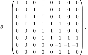
Acting on the vector~α={α1, α2, α3, α4, α5, α6, α7, α8}we can represent this element as

˜ σ =              

1 0 0 1 0 0 0 0

0 0 1 1 0 0 0 0

0 −1 −1 −1 0 0 0 0

0 1 1 1 1 1 0 0

0 0 0 −1 −1 −1 0 0

0 0 0 1 1 1 1 1

0 0 0 0 0 −1 −1 −1

0 0 0 0 0 1 1 0

              . (3.2)

Simply by matrix multiplication we then find that the order of this element is ˜h= 8. Using

an Ansatz for the deformation matrix similar to the one in [14]

θε=c0I+ (1−c0)˜σ4+i

q c2

0−c0(˜σ2−σ˜−2), c0 ∈R, (3.3)

we find that the first four constraints in (2.6) are satisfied. The ususal choice c0 = coshε

ensures that we recover the undeformed case in the limitε→0, that is the last requirement

in (2.6). Explicitly the deformation matrix resulting from (3.2) and (3.3) reads

θε=

             

1 λ0 2λ0−iκ0 3−3c0 3λ0−iκ0 3−3c0 2λ0−iκ0 λ0

0 c0 0 iκ0 2iκ0 iκ0 0 −λ0

0 0 c0−iκ0 −2iκ0 −2iκ0 −2iκ0 −iκ0−λ0 0

0 iκ0 2iκ0 c0+ 2iκ0 2iκ0 2iκ0−λ0 2iκ0 iκ0

0 −2iκ0 −2iκ0 −2iκ0 2(c0−iκ0)−1 −2iκ0 −2iκ0 −2iκ0

0 iκ0 2iκ0 2iκ0−λ0 2iκ0 c0+ 2iκ0 2iκ0 iκ0

0 0 −λ0−iκ0 −2iκ0 −2iκ0 −2iκ0 c0−iκ0 0

0 −λ0 0 iκ0 2iκ0 iκ0 0 c0

In order to achieve a more compact notation we introduced here the abbreviations κ0 =

p c2

0−c0 and λ0= 1−c0. Therefore the deformed simple roots resulting from (2.1) are

˜

α1 =α1+λ0(α2+ 2α3+ 3α4+ 3α5+ 3α6+ 2α7+α8)−iκ0(α3+α5+α7), (3.5)

˜

α2 =c0(α2+α8)−α8+iκ0(α4+ 2α5+α6), (3.6)

˜

α3 =c0(α3+α7)−α7−iκ0[α3+ 2 (α4+α5+α6) +α7], (3.7)

˜

α4 =c0(α4+α6)−α6+iκ0[α2+ 2 (α3+α4+α5+α6+α7) +α8], (3.8)

˜

α5 = (2c0−1)α5−2iκ0(α2+α3+α4+α5+α6+α7+α8), (3.9)

˜

α6 =c0α6+α4(c0+ 2iκ0−1) +iκ0[α2+ 2 (α3+α5+α6+α7) +α8], (3.10)

˜

α7 =c0α7+ (c0−1)α3−iκ0[α3+ 2 (α4+α5+α6) +α7], (3.11)

˜

α8 =c0α8−λ0α2+iκ0(α4+ 2α5+α6). (3.12)

To construct the invariant root space we compute the undeformed reduced root space ˜∆

from the orbits ˜Ωi for 1 ≤ i ≤ 8 and subsequently replace the undeformed roots in a

one-to-one fashion by their deformed counterparts. We evaluate

˜

∆ α1 α2 α3 α4 α5 α6 α7 α8

˜

σ 1;4 3;4 -2;3;4 2;3;4;5;6 -4;5;6 4;5;6;7;8 -6;7;8 6;7

˜

σ2 1;2;3;42;5;6 5;6 -3;4;5;6 3;4;5;6;7;8 -2;3;4;5;6;7;8 2;3;4;5;6;7 -4;5;6;7 4;5

˜

σ3 1;2;32;43;52;62;7;8 7;8 -5;6;7;8 5;6;7 -3;4;5;6;7 3;4;5 -2;3;4;5 2;3

˜

σ4 1;2;32;43;53;63;72;8 -8 -7 -6 -5 -4 -3 -2

˜

σ5 1;2;32;43;53;62;72;8 -6;7 6;7;8 -4;5;6;7;8 4;5;6 -2;3;4;5;6 2;3;4 -3;4

˜

σ6 1;2;32;42;52;6;7 -4;5 4;5;6;7 -2;3;4;5;6;7 2;3;4;5;6;7;8 -3;4;5;6;7;8 3;4;5;6 -5;6

˜

σ7 1;3;4;5 -2;3 2;3;4;5 -3;4;5 3;4;5;6;7 -5;6;7 5;6;7;8 -7;8

We report in this table the roots which emerge as a result of computing ˜σn(αi) with

1 ≤ n ≤ 7 and 1 ≤ i ≤ 8, where we indicate multiple occurrences by a power. Since

these root are either positive or negative it suffices to report the overall sign. For instance

we read off from the table that ˜σ3_(α

1) = α1+α2+ 2α3+ 3α4+ 2α5 + 2α6+α7+α8 or

˜

σ2(α3) =−α3−α4−α5−α6.

Next we compute the action of ˜σ± on the simple roots. We find

˜

σ−α₁ =α₁, σ˜−α₂ =α₂+α₃ = ˜σ3α₈, ˜

σ−α3 =−α3, σ˜−α4 =α3+α4+α5= ˜σ3α6,

˜

σ−α₅ =−α₅, σ˜−α₆ =α₅+α₆+α₇= ˜σ3α₄, ˜

σ−α7 =−α7, σ˜−α8 =α7+α8 = ˜σ3α2,

(3.13)

and

˜

σ+α1=α1+α4= ˜σα1, σ˜+α2 =−α2,

˜

σ+α3=α2+α3+α4 = ˜σ5α7, σ˜+α4 =−α4,

˜

σ+α5=α4+α5+α6 = ˜σ5α5, σ˜+α6 =−α6,

˜

σ+α7=α6+α7+α8 = ˜σ5α3, σ˜+α8 =−α8.

(3.14)

From (3.13), (3.14) and the above table we observed that ˜σ±αi ∈ ∆ for 1˜ ≤i ≤8, such

that ˜σ±∆ = ˜˜ ∆. Therefore replacing in the above table simple roots by deformed simple

roots,αi7→α˜ifor 1≤i≤8, consitutes a complex root space ˜∆(ε) consisting of 64 different

complex roots which remains invariant under the antilinear involutory transformations ˜σε±.

Note that in this particular case the introduction of the representative γ_i, which is often

needed to avoid overcounting, is not essential.

In order to obtain non-trivial invariant root spaces with different amounts of roots we

may select elements ˜σ ∈ W of other order ˜h. For instance we compute

˜

σ=σ1σ3σ7σ4σ6σ8, with ˜h= 4,

˜

σ=σ1σ3σ5σ7σ4σ6σ8, with ˜h= 12,

˜

σ=σ1σ3σ7σ2σ4σ6σ8, with ˜h= 20,

˜

σ=σ1σ3σ5σ7σ2σ4σ8, with ˜h= 24.

(3.15)

Generalizing then the Ansatz (3.3) to

θε=c0I+ (1−c0)˜σ˜h/4+i

q c2

0−c0(˜σ˜h/2−σ˜−˜h/2), (3.16)

yields non-trivial deformation matrices satisfying the constraint (2.6). In general we may try any element of the form

˜

σ= Y

j∈V−˜

σi

Y

j∈V˜+

σi=: ˜σ−σ˜+ (3.17)

where the product might not extend over all four odd and four even roots in V− or V+,

respectively. It is clear that this creates a large amount of possibilities. In [16] we report on how one may organise these options systematically.

4. Conclusions

We have provided a general construction procedure for invariant root spaces under an-tilinear involutory transformations. The starting point can be any element in the Weyl group. Since by definition such elements consist of products of Weyl reflections we may always bring it into a factorised form (3.17), such that each of the factors is comprised of elements related to simple roots which are not connected on the Dynkin diagram. Then

each of the factors ˜σ± will be an involution, which we can identify as an analogue to the

P-operator and subsequently we deform it to introduce the antilinear maps ˜σε±. Solving

the constraints (2.6) we construct simple deformed roots. The entire root space ˜∆(ε) may

then be constructed from the union of the reduced orbits ˜Ωi(ε). By construction it remains

invariant under the action of ˜σε± if and only if ˜σ±∆ = ˜˜ ∆.

We may then employ these spaces to investigate new types of non-Hermitian general-isation of Calogero models

H(p, q) = p

2

2 +

ω2 4

X

˜

α∈∆(˜ ε)

(˜α·q)2+ X

˜

α∈∆(˜ ε)

gα˜

(˜α·q)2, (4.1)

and investigate properties of generalised versions of affine Toda field theories decribed by Lagrangians of the form

L= 1

2∂µφ∂

µ_φ−m2

β2

ℓ

X

i=0

n0eβα˜i·φ. (4.2)

For the case ofE8 we have provided the explicit construction for the rootspaces. Based

on the conjecture that E8 plays a crucial role in the understanding and realisation of

perturbations of the Ising model it is conceivable that the complex deformed root systems serve to faciliate a systematic study of non-Hermitian perturbations of the Ising model. Generalisions to other types of spin chain and their scaled versions might be based on generalisations to other Coxeter groups.

Acknowledgments: MS is supported by EPSRC.

References

[1] A. B. Zamolodchikov, Integrals of Motion and S Matrix of the (Scaled) T=T(c) Ising Model with Magnetic Field, Int. J. Mod. Phys.A4, 4235 (1989).

[2] R. Coldea, D. E. Tennant, E. Wheeler, Wawrzynska, D. Prabhakaran, M. Telling,

K. Habicht, P. Smeibidl, and K. Kiefer, Quantum Criticality in an Ising Chain: Experimental Evidence for Emergent E(8) Symmetry, Science327, 177–180 (2010).

[3] G. von Gehlen, Critical and off-critical conformal analysis of the Ising quantum chain in an imaginary field, J. Phys. A24, 5371–5399 (1991).

[4] O. Castro-Alvaredo and A. Fring, A spin chain model with non-Hermitian interaction: The Ising quantum spin chain in an imaginary field, J. Phys.A42, 465211 (2009).

[5] E. Wigner, Normal form of antiunitary operators, J. Math. Phys. 1, 409–413 (1960). [6] C. M. Bender and S. Boettcher, Real Spectra in Non-Hermitian Hamiltonians having PT

Symmetry, Phys. Rev. Lett. 80, 5243–5246 (1998).

[7] C. M. Bender, Making sense of non-Hermitian Hamiltonians, Rept. Prog. Phys.70, 947–1018 (2007).

[8] A. Mostafazadeh, Pseudo-Hermitian Quantum Mechanics, arXiv:0810.5643 . [9] M. Znojil and M. Tater, Complex Calogero model with real energies, J. Phys. A34,

1793–1803 (2001).

[10] M. Znojil and A. Fring, PT-symmetric deformations of Calogero models, J. Phys.A41, 194010(17) (2008).

[11] M. A. Olshanetsky and A. M. Perelomov, Classical integrable finite dimensional systems related to Lie algebras, Phys. Rept. 71, 313–400 (1981).

[12] G. Wilson, The modified Lax and two-dimensional Toda lattice equations associated with simple Lie algebras, Ergodic Theory and Dynamical Systems1, 361–380 (1981).

[13] D. I. Olive and N. Turok, The symmetries of Dynkin diagrams and the reduction of Toda field equations, Nucl. Phys.B215, 470–494 (1983).

[14] A. Fring and M. Smith, Antilinear deformations of Coxeter groups, an application to Calogero models, J. Phys. A43, 325201(28) (2010).

[15] P. E. G. Assis and A. Fring, From real fields to complex Calogero particles, J. Phys.A42, 425206(14) (2009).