Cognitive Control Systems in Steel Processing Lines for Minimised Energy Consumption and Higher Product Quality (Cognitive Control) : Final Report

Cognitive control systems

in steel processing lines

for minimised energy

consumption and higher

product quality

(Cognitive Control)

Research and

Innovation

EUR 27317

EUROPEAN COMMISSION

Directorate-General for Research and Innovation Directorate D — Key Enabling Technologies Unit D.4 — Coal and Steel

E-mail: [email protected] [email protected]

Contact: RFCS Publications

European Commission

Research Fund for Coal and Steel

Cognitive control systems in steel processing

lines for minimised energy consumption and

higher product quality

(Cognitive Control)

Andreas Wolf, Martina Thormann, Mohieddine Jelali

VDEh-Betriebsforschungsinstitut GmbH (BFI)

Sohnstraße 65, 40237 Düsseldorf

Björn Sjögren

Swera MEFOS AB (MEFOS)

Arontorpsvägen 1, SE-971 25 Luleå (Sweden)

Jürgen Bathelt, Peter Förster

ArcelorMittal Eisenhüttenstadt (AMEH)

Werkstraße 1, 15872 Eisenhüttenstadt (Germany)

Luis Felipe Recalde, Reza Katebi, Hong Yue

Industrial Control Centre (ICC) University of Strathclyde

16 Richmond Street, GB-Glasgow G1 1XQ (UK)

Wolfram Gerlach

ThyssenKrupp Nirosta (TKN)

Oberschlesienstraße 16, 47807 Krefeld (Germany)

Grant Agreement RFSR-CT-2010-00037 1 July 2010 to 31 December 2013

Final Report

Directorate-General for Research and Innovation

LEGAL NOTICE

Neither the European Commission nor any person acting on behalf of the Commission is responsible for the use which might be made of the following information.

The views expressed in this publication are the sole responsibility of the authors and do not necessarily reflect the views of the European Commission.

More information on the European Union is available on the Internet (http://europa.eu).

Cataloguing data can be found at the end of this publication.

Luxembourg: Publications Office of the European Union, 2015

Print ISBN 978-92-79-49482-6 ISSN 1018-5593 doi:10.2777/642342 KI-NA-27-317-EN-C PDF ISBN 978-92-79-49074-3 ISSN 1831-9424 doi:10.2777/90680 KI-NA-27-317-EN-N

© European Union, 2015

Reproduction is authorised provided the source is acknowledged.

Printed in Luxembourg

Printed on white chlorine-free paper

Europe Direct is a service to help you find answers to your questions about the European Union

Freephone number (*):

00 800 6 7 8 9 10 11

Contents

1 Final Summary 5

2 Objectives of the project 13

3 Description of activities and discussion 15

3.1 WP 1: Development of methods for continuous control performance assessment . . . . 15

3.1.1 Task 1.1: Analysis of existing control loops and identification of tuning

param-eters and data needs [ALL PARTNERS] . . . 15

3.1.2 Task 1.2: Development and implementation of databases [AMEH, MEFOS, TKN] 20

3.1.3 Task 1.3: Development offline test of automatic control-loop performance

eval-uation methods [ALL PARTNERS] . . . 25

3.2 WP 2: Development of techniques for the automatic diagnosis of root causes of poor

control performance . . . 50

3.2.1 Task 2.1: Development of methods to determine the root causes of performance

losses detected in the control loops [ICC, BFI] . . . 50

3.2.2 Task 2.2: Synthesis of promising diagnose procedure to be applied to the

spe-cific loops considered[all] . . . 60

3.2.3 Task 2.3: Developement of the diagnosis of root cause reporting systems[MEFOS,

AMEH; ICC, TKN] . . . 81

3.3 WP 3: Development of methods for automatic tuning by generating optimal setup

pa-rameters and controller settings . . . 83

3.3.1 Task 3.1: Development of strategies and methods for re-tuning controllers [ALL

PARTNER] . . . 83

3.3.2 Task 3.2: Working out decision masking concept and supervision procedures

for automatic re-tuning [ALL PARTNERS] . . . 101

3.3.3 Task 3.3: Procedure simulation of automatic re- tuning of the control loops,

comparison of selected methods [ALL PARTNERS] . . . 104

3.4 WP 4: Implementation„ interface programming and on-site implementation of

auto-matic control optimization techniques . . . 109

3.4.1 Task 4.1: Development and test of the SCADA interface to the performance

and fault monitoring software [ICC] . . . 109

3.4.2 Task 4.2: Implementation of procedures adapt and verify performance

assess-ment and automatic root-cause diagnosis results [ALL PARTNERS] . . . 111

3.4.3 Task 4.3: Implementation of continuous monitoring and automatic retuning

decision making procedures [BFI, MEFOS, AMEH, TKN] . . . 113

3.5 WP 5: Final testing and evaluation of developed tools and systems . . . 119

3.5.1 Task 5.1: Methods and systems for demonstration at the galvanizing lines and

linked pickling/cold rolling mill at the ArelorMittal Eissenhüttenstadt [AMEH, BFI] . . . 119

3.5.2 Task 5.2: Methods and systems for demonstration at (stainless steel) bright

annealing lines at ThyssenKrupp Nirosta [TKN, BFI] . . . 122

3.5.3 Task 5.3: Methods and systems for demonstration at annealing lines of MEFOS

[MEFOS] . . . 135

3.5.4 Task 5.4: Evaluation of final results and recommendations [ALL PARTNERS] 138

4 Conclusions 141

6 Acronyms and Nomenclature 145

8 List of Figure 150

9 List of Tables 155

1 Final Summary

WP 1: Development of methods for continuous control

performance assessment

Task 1.1: Analysis of existing control loops and identification of tuning parameters and data needs [ALL PARTNERS]

ICC and BFI focused on identifying common sources of poor performance in hot rolling mills, an-nealing and galvanizing processes. The identified root-causes were in this case process, transition or scheduling strategies, variable operating points, use of SISO controllers, sensor and actuator faults, model uncertainties and internal/external disturbances. AMEH was interested in assessing and im-proving the control systems in two processing plants: the gauge control system at the hot strip mill, including AGC, monitor control, mass flow control and looper control and the strip guiding controls in the annealing lines. TKN runs several annealing lines. After Analysing the potential of their furnaces, it was decided to choose the annealing furnace ”KL3”; MEFOS chose the annealing furnace ”KBR” at Outoumpu Aveta.

Task 1.2: Development and implementation of databases [AMEH, MEFOS, TKN]

From the chosen aggregates process data was selected for further performance analyses. Within these processes the strip speed was significantly influenced by acceleration and deceleration. This meant that strip-length samples were not equally distant in time. This was motivating performance evaluation in a length-based setting rather than in a time-based setting and also avoided the need to estimate any time delay, as the distance from actuator to sensor is constant in the length-based scenario. After these pre-processing steps, the data of each coil was analysed.

Task 1.3: Development offline test of automatic control-loop performance evaluation methods [ALL PARTNERS]

The results of Task 1.1 were used to choose appropriate Control Performance Assessment (CPA) methodologies in Task 1.3. Continuous offline methods were implemented by BFI and ICC for time-delay estimation, detection of nonlinearities and ANalysis Of VAriance (ANOVA) over Minimum Vari-ance (MV)-CPA. New methodologies for controller only pre-assessment, monitoring of nonlinearities and systematic diagnosis were developed. The methods were tested on SISO systems and cold rolling mill data, hot rolling mills, annealing furnaces in cooperation with MEFOS, AMEH and TKN.

ICC provided new methods for controller pre-assessment. The pre-assessment was achieved by com-bining recursive closed-loop subspace identification with QR decomposition, wavelet decomposition for feature extraction and a Model Predictive Control (MPC) benchmark designed with the extracted deterministic features of the original data (or filtered data) from the wavelet decomposition. QR de-composition was used for process identification to avoid ill-conditioned problems on the algorithm due to none or poor persistent excitation. A new methodology for monitoring of nonlinearities was also developed for Task 1.3. The methodology used State-Dependent (SD) model identification to identify any existing nonlinearities and a Filtering and CORrelation (FCOR) scheme for Control Performance Monitoring (CPM)

introduced by BFI to separate the time spans automatically. The methods are based on the detection of steady and non-steady states parts of the measuring signal. Furthermore, a static energy index was introduced as the ratio between energy of the strip and the fuel. If this index excites a limit, there are hints to malfunction in the furnaces, demonstrated in Task 5.2. Besides the well-known Harris index, the idle index for detection of sluggish controller was introduced and the Visioli index added. The aim of the methodology is to evaluate an abrupt load disturbance response if the tuning of the adopted PI controller guarantees good load-disturbance rejection performance.

WP 2: Development of techniques for the automatic diagnosis of

root causes of poor control performance

Task 2.1: Development of methods to determine the root causes of performance losses detected in the control loops [ICC, BFI]

The diagnosis algorithm developed here comprised the following steps:

• Pre-analysis of nonlinearity and dead-time estimation.

• Feedback controller assessment.

• Process and disturbance assessment.

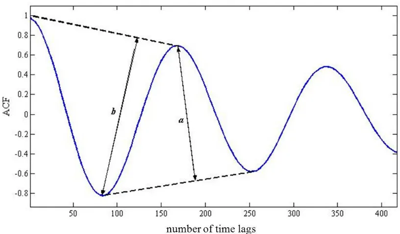
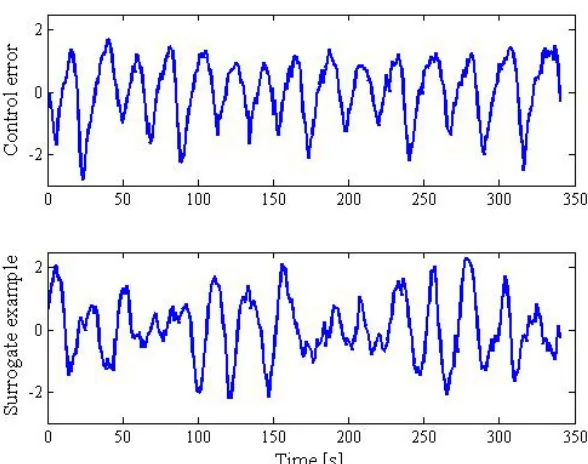
For this task, BFI added an extra method for oscillation detection based on regularity of zero-crossings of the autocorrelation function (ACF) of the process data. In addition, similar techniques have been studied, called the decay ratio approach of the auto-covariance function. Furthermore, nonlinearity de-tection based surrogates analysis was added. Finally, BFI has presented methods to detect stiction as the root-cause of oscillation.

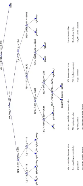
The methods implemented by ICC in Task 1.3 were combined into a decision tree approach to pre-dict root-causes of poor performance. Each methodology was expressed as a metric. Metrics extracted from a nominal data set (or data with the best performance) were used as decision rules in the decision tree. The resulting decision tree was fed with new data and a possible root-cause is predicted.

Task 2.2: Synthesis of promising diagnose procedure to be applied to the specific loops considered [all]

A new CPM and diagnosis methodology was developed for Tasks 2.2 to tackle multivariable processes. The methodology combines recursive closed-loop subspace identification, MPC benchmark, wavelet decomposition, Kernel Principal Component Analysis (PCA) for faults monitoring and angle-classifiers for root-cause identification. The CPA benchmark was designed as in controller pre-assessment with the addition of the stochastic features to improve the MPC design. MPC benchmark was also chosen for its ability to assess input variability or input energy. Root-causes in data were monitored at several

frequencies through the wavelet decomposition. Statistical metrics such as Hotteling’s statistic (T2) and

Square Prediction Error (SPE) were used for monitoring in all the decomposed frequencies. Identifica-tion of root-causes was achieved by determining the angle between the Principal Components (PC’s) of a detected abnormality in the data against known principal components from pre-identified root-causes. The identification was enhanced by applying other data features such as amplitude of the statistical metrics and PC’s’ worst directions.

This method was applied on a multivariable case study and on the data of the annealing furnace MEFOS partner provided. This has lead to further investigations of the control loops of the MEFOS partner, es-pecially on the performance due to thickness jumps and analyses of model used within the control loop. Furthermore, this method was presented by MEFOS to supervise temperature measurement based on PCA analyses.

has been found to be oscillating, the most probable origin was assumed valve stiction. However, non-linearity had to be checked as a possible source of oscillation. A stiction detection method was then applied and its level estimated. It was tested with the simulation and diagnoses developed in the project.

Task 2.3: Development of the diagnosis of root-cause reporting systems[MEFOS, AMEH; ICC, TKN]

A structure of a performance monitoring and root-cause diagnosis reporting was proposed. It has been inspired by the structure used in the cpmPlus Loop Performance Manager of ABB, but extended by the new methods and features developed within this project.

WP 3: Development of methods for automatic tuning by

generating optimal setup parameters and controller settings

Task 3.1: Development of strategies and methods for re-tuning controllers [ALL PARTNER]

The continuous annealing furnace which was investigated by Swerea MEFOS reheats steel strips of various steel grades, thicknesses and surface finish. Thicker strips require more time in the furnace, and the optimal reheating parameters were calculated by temperature prediction software that takes data from furnace instrumentation and operator input for factors including the furnace wall temperatures, the strip thickness and emissivity, fuel flow rates, etc. The model included the furnace geometry which is a fixed parameter. The dominant type of heat transfer at these high temperatures is radiative, so the reheating is particularly sensitive to the surface emissivity. One potential source of sub-optimal control loop performance was the interaction between the radiative heat transfer model in the strip temperature predictor and the strip emissivity data. The strip emissivity should have normally increased with in-creasing temperature, since an oxidized steel surface has a higher emissivity than a blank steel surface. There were also strips with oxidized surfaces where the change in emissivity of the surface through the furnace was not known.

The University of Strathclyde focused on the development of the following three methodologies: Su-pervisory MPC gain compensation, "one shot" gain compensation based on covariance control, and iterative gain compensation. The methodologies required estimation of the process dynamic matrix and noise matrix. The estimation was carried out using a recursive closed-loop subspace identification method based on process data only. The Control Performance Assessment (CPA) index was used to trigger the re-tuning process as well as the stopping mechanism. It wass expected that the re-tuning process starts after improper tuning of the controller which had been identified as the main source of poor performance by a diagnosing method.

Task 3.2: Working out decision masking concept and supervision procedures for automatic re-tuning [ALL PARTNERS]

A principal decision procedure for carrying out the right measures for improving the performance of a control system was provided. A continuous CPM system indicated whether the control performance has been acceptable, i.e. meets the required specification in terms of standard deviation or other measures, product quality, energy consumption or even safety. This level wass thus more related to the direct economical performance of the plant shown later in Task 5.2. When proceeding with the performance analysis, the current performance is compared to that of the selected benchmark, to find out whether the installed controller performed well under the current process condition.

Furthermore, strategies for variation of controller parameters for automatic re-tuning PI and PID con-troller were given. Iterative concon-troller tuning required the specification of a proper step size for each controller parameter, usually given as percentage. Cautious adjustments to the controller parameters were necessary to guarantee closed-loop stability and performance improvement. There were many strategies for varying the controller settings in each iteration. Some of them are described in the follow-ing, including their strengths and weaknesses. Basically, a large step size helps to reduce the number of iterations required but may increase the risk to converge to controller parameters far from the optimum.

The simplest approach is to vary only the proportional gain KP unless the existing controller is

ei-ther too sluggish or too aggressive. In such cases, the integral timeTI can also be changed (but only one

parameter at a time). Otherwise, the variation ofKp, should only lead on to a value near the optimum,

and then a "fine tuning" could be done by slight variation ofTI. The simultaneous adjustment of the

controller settings, i.e. decreasingKp, and increasingTI (and possibly decreasing TD) when the

con-troller is aggressive and vice versa in the case of a sluggish concon-troller, is the fastest method to find the optimum tuning. However, this approach is not transparent in practice and should only be considered by well-qualified users. The third method is based on successive variation of the control parameter. In this approach, the proportional term is tuned first until the highest performance index value is reached. This is followed by tuning the integral time and possibly derivative time, which may lead to further

improve-ment in Harries indexη. Although this approach usually takes more iterations than the simultaneous

strategy, it is highly recommended in practice because of its transparency.

Task 3.3: Procedure simulation of automatic re- tuning of the control loops, comparison of selected methods [ALL PARTNERS]

The University of Strathclyde compared its three developed methods with the Visioli’s method. Four

metrics were used to validate the improvement: controller performance assessment, idle indexIi, area

indexIa and output index Io. A simple SISO system with PI control was used as a benchmark. The

results show the calculated controller parameters of the four methods. Note that supervisory method and covariance control method find the new controller parameters at the first iteration since they are "one-shot" solutions. In practice, the supervisory method sampled the process at a different sampling rate compared to the local controllers. The re-tuning procedure had consequently taken longer. The iterative methodologies took 4 and 3 iterations respectively. The modified Iterative Feedback Tuning (IFT) method took less than the Visioli method since the latter is based on small percentage variations of the controller parameters rather than an optimal recursion. It was important to take into account that the modified IFT method can take higher numbers of iteration according to the complexity of the process. In general no big differences among the performance of the method were found.

WP 4: Implementation„ interface programming and on-site

implementation of automatic control optimization techniques

Task 4.1: Development and test of the SCADA interface to the performance and fault monitoring software [ICC]

The University of Strathclyde ombined all the methodologies used and developed by the ICC into a MATLAB software tool. Supervisory Control And Data Acquisition (SCADA) functionality was added to the software tool through the Object linking and embedding Process Control (OPC) toolbox. OPC is a MATLAB toolbox developed to provide connectivity, directly from MATLAB and Simulink, between OPC clients running software applications and any OPC Data Access (DA) and Historical Data Access (HDA) compliant servers. The toolbox allows reading, writing and logging OPC data from devices such as distributed control systems, SCADA systems and programmable logic controllers that conform to the OPC Foundation DA standard

Task 4.2: Implementation of procedures adapt and verify performance assessment and automatic root-cause diagnosis results [ALL PARTNERS]

In this task several method tools were developed to implement performance assessment and root-cause diagnostics. BFI and TKN developed a simulation and diagnostic tool for annealing furnace KL3. It contains a simulation tool of the dynamic behaviour of the furnace and controller; a fault injection tool to simulate the reaction of the furnace and controller on faults in sensor and actuator; a diagnostic tool to analyse the performance and cause of possible degradation. Data from simulation or coming from the plant were analysed. The results are shown in Task 5.2. A similar tool has been adapted for the annealing line VZA2 at AMEH. MEFOS assisted AVESTA by setting up monitoring and diagnoses for the annealing furnace KBR.

Task 4.3: Implementation of continuous monitoring and automatic retuning decision making procedures [BFI, MEFOS, AMEH, TKN]

In simulation and diagnosis tools by BFI for the KL3 of TKN, a set-up optimisation tool was also integrated. Additionally, it provided a tool to optimize the set-point of the furnace controller. The set-point was optimized in such a way that the deviations from the desired strip temperature caused by thickness changes and strip speed changes were reduced. This lead to more homogeneous strip quality. In the tool for AMEH BFI some iterative controller re-tuning features were added, based on the relative damping index. The results have been described in Task 5.1. MEFOS assisted AVESTA by setting up monitoring and controller retuning based on MPC methods.

WP 5: Final testing and evaluation of developed tools and

systems

Task 5.1: Methods and systems for demonstration at the galvanizing lines and linked pickling/cold rolling mill at the ArelorMittal Eisenhüttenstadt [AMEH, BFI]

In this task controller performance analysis, root-cause analysis of performance degradation and auto-matic re-tuning using the tools, provided by BFI, was demonstrated at the galvanizing line VZA2 of AMEH. First results showed that some controllers were switched off quite often by the operators. When analysing these controllers, insufficient performance was detected. A further analysis showed that the reason for degradation wass due to oscillation, but stiction as a cause for oscillation has been excluded.

After some further investigation by AMEH, it was found that the strip, which reaches a temperature of 300 C at the end of the RTHA zone, did not show any or at least slight oscillations. Still, if the strip

reached only 180◦C in this zone, the strip started to oscillate. Therefore, an additional temperature

mea-surement and controller was installed. The strip temperature at the end of this zone was kept constant

Iterative tuning was applied to one controller which showed insufficient performance but no oscilla-tion. After two iterations, a significant performance increase was achieved.

Task 5.2: Methods and systems for demonstration at (stainless steel) bright annealing lines at ThyssenKrupp Nirosta [TKN, BFI]

In this task, the control performance and root-cause analysis of performance degradation using the tools developed in this project was demonstrated at the bright annealing line of TKN. First, the performance of the furnace was analyzed using MIMO methods provided by ICC.

Afterwards a root-cause analysis based on Furnace Simulation Diagnosis Tools was carried out. Offset of temperature measurement could be detected and lead to asymmetric load distribution in the furnace. Counter measures were implemented and tested. In the performance analyses, it was pointed out that

the violation ofT2at high scales could be related to sources of oscillation. To verify this assumption,

the behaviour of the temperature control at changes in the thickness was investigated. This lead to improvement of the reaction of the furnace controller due to thickness changes, reducing costs signifi-cantly.

Task 5.3: Methods and systems for demonstration at annealing lines of MEFOS [MEFOS]

In this task, the control performance and root cause analysis of performance degradation using the tools developed in this project were demonstrated at the annealing lines of MEFOS. First the performance of the furnace was analysed. Then the root-cause of the performance degradation was carried out. Based on a number of temperature measurements using DATAPAQ and thermocouples attached to the strip, it was clearly detected that there is a deviation between the calculated and the measured temperature. By further analysing the oxygen level in the furnace, it was concluded that false air was leaking into the furnace. After calculating the energy balance of the furnace, it was detected that the gas radiation model for the oxyfuel combustion has not been elaborated correctly.

Task 5.4: Evaluation of final results and recommendations [ALL PARTNERS]

The analyses and tuning methods applied in this project had several effects on the investigated plant: the detection of sensor fault, in this case an offset on the temperature measurement, saves approx. 1.3GWH per year and yields to significant cost saving. Furthermore, the overall benefit of the measures applied

in this project at TKN lead to a reduction of out-tolerance of grain size of about 150.000ea year.

Generally, before applying performance analyses, root-cause analyses and re-tuning wass recommended: at first the verification of data had to be consistent, otherwise this could have lead to false interpreta-tion of the later analysis steps. The first analysis checked whether the signal is “alive” and the second whether the analysed controller is really switched on or off. Then the data of interest was selected. In order to avoid unnecessary metrics calculations, the controller has been assessed to rule out improper tuning or inadequate control structure first. Improper tuning was considered the main cause of poor performance.

There is not a database of general root-causes in steel processing lines. Most of the methodologies for diagnosis are based on the identification of new data features against known data features. Even if the accuracy of a given methodology identifies new abnormal data features, they can not be linked to a known or new root-cause. Diagnosis for steel processing lines is at the stage where many destructive tests have to be carried out in order to identify possible root-causes of poor performance. It is important to keep in mind that some root-causes have shared effects. The identification of a given root-cause may need several tailored diagnosis methodologies or monitoring at different frequencies.

2 Objectives of the project

The aim of the proposal was to create cognitive automation systems with the capabilities of automatic monitoring of control performance, self-detection and automatic diagnosis of faults (sensors, actuators, controller) and self-adaptation in control system environments to optimise the product quality and min-imise energy consumption in steel lines (cold rolling mills, annealing, galvanising) during the whole life cycle. In details, the project objectives were:

• New technologies for continuous online performance assessment of complex setup and control

systems in different steel processing lines were developed.

• Methods for automatic diagnosis of root-causes of poor control performance were developed.

• Economical criteria, particularly energy consumption were explicitly considered in the control

performance metrics and monitoring and re-tuning algorithms.

• An integrated control data system, containing all information about performance, re-tuning

ac-tions and loop testing or maintenance advices were developed.

• Strategies and procedures for integrating the automatic control improvement into the automation

systems and the maintenance practices for different finishing lines were developed.

• The developed methods were implemented and transformed into tailored software tools working

automatically and continuously with the control data system.

• The supervised automatic control performance optimization methods and systems and the use of

3 Description of activities and discussion

3.1 WP 1: Development of methods for continuous control

performance assessment

The main objectives of this WP were:

• Detailed definition of requirements for the control systems to be monitored and tuned at the

different target mills were carried out.

• Databases needed for the monitoring and tuning were provided

• Critical review of the control performance assessment technology in the steel processing area and

fields was carried out.

• Different methods of control performance assessment were investigated and compared.

• New methods towards continuous and online control performance monitoring, explicitly

consid-ering energy consumption were developed.

• A set of rules for alert generation and the structure of the assessment reporting were worked out.

• Selected methods to data gathered from the different plants were applied .

3.1.1 Task 1.1: Analysis of existing control loops and identification of tuning parameters and data needs [ALL PARTNERS]

In the following, a short study of the control loops in steel processing lines is described first, with the aim of identifying sources of performance degradation and critical tuning parameters as well as assessing possible causes for poor loop performance. Then, an analysis of the industrial control systems to be evaluated and improved within the project is presented, (being deliverable D1.1).

There are various sources in a steel line that may degrade the performance of the processes and sub-processes, e.g.:

• Type of processes. Metal processing lines are generally divided into processes. Each sub-process modifies the properties of the product. These changes cannot be tracked automatically.

• Transition or scheduling strategies. Every single piece of the final product depends on the customer-order specifications. Variations in product properties can be traced back to the start-ing point, consequently, delays of production, continuity and idle times must be scheduled.

• Variable operating points. The whole steel line is set-point-dependent. To obtain customer-order specifications, every sub-process uses individual setups [Pit11]. Models for setup variations are highly nonlinear and difficult to implement.

• SISO controllers. It has been reported that most of the sub-processes have poorly tuned SISO controllers with a half-life of about six months [Jel06b].

3.1.1.1 Selection of target plants and first analysis at AMEH

AMEH was interested in assessing and improving the control systems in two processing plants:

1. Gauge control system at the hot strip mill, including AGC, monitor control, mass flow control and looper control.

2. Strip guiding controls in the annealing lines.

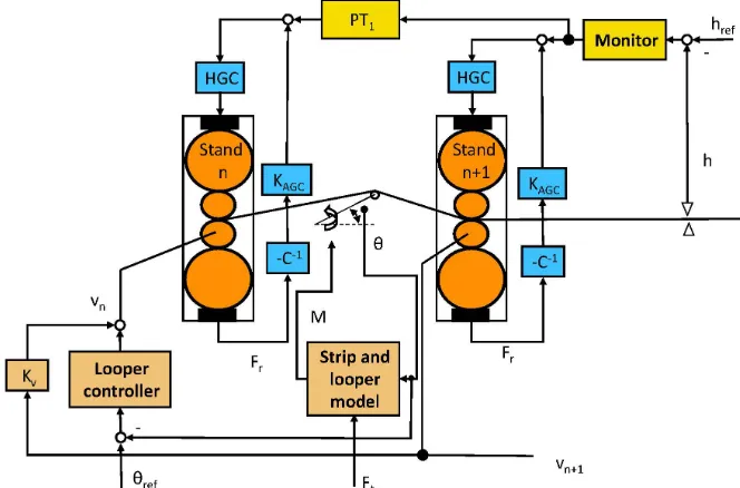
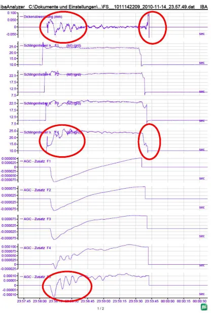
Figure 3.1 shows the structure of the gauge control at AMEH’s hot strip mill. In figure 3.2 some variables from the control system are illustrated. It can be observed that the control performance was not satisfactory due to the possible root causes: oscillating loops, inaccuracies in the strip or time delay model or mutual interaction between some control loops. This control behaviour was thus analysed using the methods developed in Task 1.3 and the root-causes diagnosed by the techniques developed in Task 2.1.

Figure 3.1:Structure of the gauge control at AMEH’s hot strip mill

A first analysis of the current control structure showed that it had the configuration depicted in figure 3.3. The implemented structure looked like, but was no Smith predictor. This is not – at least from a theoretical viewpoint – the favorable structure, and thus may lead to performance problems. The modification of the control structure hence improved the quality of the strip thickness.

Figure 3.3:Basic control structure as currently implemented at the hot strip mill

3.1.1.2 Selection of target plants and first analysis at TKN

TKN possesses several annealing lines; their features are given in Table 3.1. The optimisation potential of the annealing lines within this project was analysed with the aim to choose the line with the biggest potential benefit. Finally, two annealing lines (KL 3 and GBL 3) were chosen for further elaboration.

Figure 3.4:Maximum load comparison of annealing lines KL 3 and GBL 3

Table 3.1:Features of the analysed process lines at TKN

Process line

Remaining term

Last control system revamping

Docum. control system

Data in DB

Grain size measur.

WL 2 Ca. 4 years before 1980 - -

-KL 2 Ca. 5 years 1999 available -

-GBL 3 2007 available available

-KL 3 2002 New construction,

2010 Tension control

available available available

In Fig. 3.4, the relative frequencies of maximum loads of each heating zones were compared. The last zone of GBL 3 had a maximum load in 38% of production time in comparison to 20% of the KL 3’s last zone. In total, KL 3 heating sections operated less often with maximal load. This allowed the controller more often to work as it was designed, and thus an optimal tuned/structured controller became more important. For this reason, KL 3 was chosen to be evaluated and improved within this project.

3.1.1.3 Selection of target plants and first analysis at MEFOS

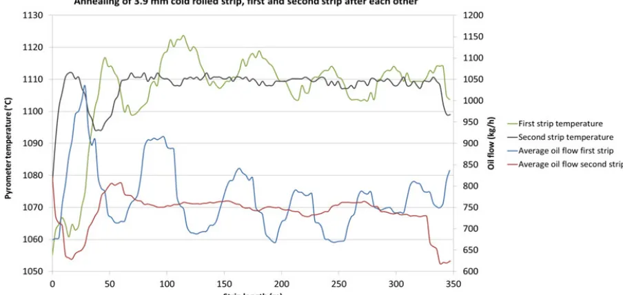
Outokumpu Avesta was interested in improving the process control capability of their annealing line, KBR. The layout of the annealing furnace at Outokumpu Stainless, Avesta is shown in figure 3.5. The furnace consists of 2 parts divided into 6 zones; zone 1 and 2 are located in the first part and zones 3, 4, 5 and 6 are located in the second part. The steel strip travels across the zones via a support roll between the 2 furnace parts at the end of zone 2. There are a total of 35 burners, 25 thermocouples and 5 pyrometers are used to control the furnace and steel strip temperature. The furnace is 39 m long

with an interior width of 4 m. Strips up to 2 m wide are annealed at temperatures of approx 1100◦C

and the strip thickness vary between 1.5 and 12.8 mm, both hot and cold rolled strips are treated. The maximum speed is set by the pickling station at 24 m/min. The mass flow is generally aimed at 80 tonnes/hour for cold rolled strips and 96 tonnes/hour for hot rolled strips. The cold rolled strips are generally more resistant to the heat transfer because of the lower emissivity of the relatively oxide free surface, necessitating a lower mass flow.

The coiled strips are welded together in sequence to create a continuous process. There is a strip buffer on the entry side so the process can be uninterrupted when welding the strips together. The strips are annealed in the annealing furnace and then quickly cooled with air and water to create the desired material properties.

Figure 3.5: Location of the thermocouples and the pyrometer used in the following examples. Distance between thermocouples is around 5 m

The temperature in the furnace is predicted and controlled by DynaMIC, software, which is partly

based on the Swerea MEFOS software STEELTEMPR. The prediction software has been developed by

Prevas and it utilizes the incoming strip and furnace parameters to determine the strip temperature and how many and how much to fire the set of burners in each zone, each 0.5 m of the strip is calculated and the predictions are made zone per zone. The prediction software is supported by the furnace pyrometers that can also be used as controls alone, or partly, together with the calculations.

is chosen with similar thickness to the actual strip if possible but it is normally thicker, at about 4 mm. The ends are welded to each other to form a continuous strip resulting in a reoccurring 13 m section that will consequently be cooler than the actual, most often thinner, strip. The furnace is controlled only by the DynaMIC control software when the 13 m section passes the furnace as the pyrometers react heavily to the colder strip.

3.1.2 Task 1.2: Development and implementation of databases [AMEH, MEFOS, TKN]

The databases (being deliverable D1.2) required to acquire and store the signals necessary for the con-tinuous control performance monitoring of the selected control loops were adapted or developed. In-terfaces between the databases and the existing automation data buses were also established. Hardware required for the databases and to run the control loop performance evaluation and automatic re-tuning systems was installed at the plants and interfaced to the automation systems.

3.1.2.1 Databases established at hot strip mill of AMEH

All signals of the hot strip mill of AMEH that may be needed for control performance assessment were recorded over three months, consisting of approximately 14000 coils:

• Strip thickness / thickness deviation

• Strip width / width deviation

• Strip flatness coefficients

• Strip wedge

• Temperatures / temperature deviations (exit F1, exit F7, entry coiler)

• Rolling forces, torques

• Rolling speeds

• Looper angles, tensions

• Roll gap positions

• Work roll bending forces

• Shifting (CVC) positions

• AGC offsets

• Strip length

• Tilting positions

Because metal rolling is a batch process, where time between two coils or passes is in the range of minutes, control performance evaluation was usually carried out offline after completing the batches and coil by coil. Before the performance of the controller can be analyzed, the following pre-processing steps had to be carried out:

• Test on plausibility.

• Down-sampling.

Figure 3.6:Pre-analysis of hot strip gauge control signals

After these pre-processing steps, the data of each coil was split up into ranges for the different rolling phases, e.g. setup, control-on, etc.; see Fig. 3.7. Then the performance of the thickness controller was analyzed. For the calculation of the Harris index, the thickness deviation data was taken; for the Visioli index, the manipulating variable (AGC offset) data was needed supplementary.

3.1.2.2 Databases established at the galvanizing line of AMEH

All signals of the galvanizing line of AMEH that maybe needed for control performance assessment were recorded over three months:

• furnace temperature for each furnace zone

• strip temperature

• strip speed

• strip width

• strip thickness

• strip position for each furnace zone

• position of the steering for each furnace zone

The same pre-processing steps were carried out as for the hot strip mill data.

3.1.2.3 Databases established at the annealing lines of TKN

Data interfaces and acquisition systems were checked for the availability of process data required for automatic control performance monitoring. Data and parameter types and formats were agreed on during meetings and discussions with the plant personnel. Data was stored and transferred to BFI per remote access, so that analysis was possible when requested. Data from the annealing line KL3 was gathered over a period of some months and analyzed using the CPM routines developed in MATLAB. Figure 3.8 shows a typical example of data measured and analyzed within the project.

A first analysis revealed the importance of plausibility checks and the requirements for many coils were merged to have an appropriate length of data, suitable for performance analysis. Otherwise the

data lengths would have been too short and the results unreliable, due to the sampling time ofTs=10s

as can be seen below.

3.1.2.4 Databases established at the annealing furnace of Outokumpu Stainless (MEFOS)

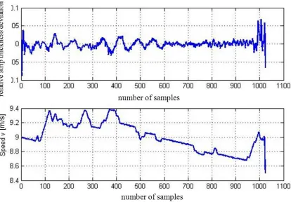
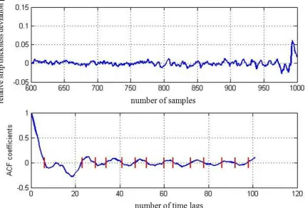
Data interfaces and acquisition systems were checked for the availability of process data required for automatic control performance monitoring. Data and parameter types and formats were agreed on during meetings and discussions with the plant personnel. Data was stored and transferred to MEFOS. The data was collected from 17 consecutive strips in the annealing furnace. Sampling was done with a 10 s cycle time and the whole record was 7 hours and 26 minutes long. Of the strips that were annealed during this time the first 7 were hot rolled and the following 10 cold rolled.

12.8 mm was the initial strip thickness followed by thinner and thinner strips in steps of 0.1–2 mm down to 1.5 mm as the thinnest.

The large number of parameters and responses made the visualization of the data difficult. The following graphs thus only represent chosen parts. For example figure 3.9 displays the effect of the strip change, in this case from 1.5 up to 2 mm cold rolled strips. The change was registered at 06:32:50 and the first part of this new strip reached the zone 6 pyrometer at approximately 06:35:50, the cooler 13 m holding strip was clearly distinguishable because of the rapid drop in pyrometer temperature at 06:35:20.

3.1.3 Task 1.3: Development offline test of automatic control-loop performance evaluation methods [ALL PARTNERS]

Software tools (being deliverable D1.3) for automatic performance evaluation of control loops requires at least three steps:

1. Data pre-processing for control performance monitoring

2. Pre-analysis of the process to look for system nonlinearities, oscillations, variations in time de-lays, etc.

3. Calculation of adequate performance metrics.

4. Identification of sources of poor performance.

Without lack of detail, these four steps provide a comprehensive procedure to assess process perfor-mance as well as controller perforperfor-mance.

This task took longer than planned, because some extra ideas to detect sensor faults based on energy index for furnaces have been added. These ideas have been motivated by practical experiences at the annealing furnace of TKN.

3.1.3.1 Data pre-processing for control performance monitoring

For using the Harris index [Har89] one has to select steady-state data for the benchmarking of control loop performance. In practical application, for instance, when analysing the thickness control of a hot strip mill, there are large amounts of measurement data to be analysed, containing also periods of steady and non-steady-states. It is quite a difficult task to separate time periods manually, hence methods are introduced to separate the time spans automatically.

The methods are based on the detection of steady and non-steady states parts of the measuring signal.

Batch steady state detection. [Rhi95] published a steady-state index based on the ratio of the variance of the control error. In steady-state, the control error is an independent stochastic noise with

mean value zero. The steady-state indexRis defined as follows:

R=σ

2

e1

σ_e2₂ (3.1)

with the variance of the control error; see also (Figure 3.10):

σe21= 1 2·(n−1)·

n

∑

i=l

(e1,i)2 (3.2)

and variance of the difference between the current and last control error

e₂,i = e1,i−e1,i−i (3.3)

σe22 =

1 2·(n−1)·

n

∑

i=l

(e₂,i)2 (3.4)

For a closed-loop control in steady-state the steady-state indexRis nearly 1. If the control loop is

non-steady-state, the value ofRincreases as shown in figure 3.11 for the thickness control. The drawback

of steady-state indexRis that the control error has to be stored for computation of the index.

Recursive steady state detection Coa [Cao95] published another variant of this steady-state

indexR. The steady-state indexRf uses the same deviations of the control error e1, e2 (Figure 3.10).

[Cao95] additionally uses for Rf a filter to avoid storing past data of control error for calculating the

variance.

Rf = σ_e2_1,f,i

Figure 3.10:Control error

Figure 3.11:Steady-state detection

with filter for the variance of control error

σe21,f,i=λ·(e1,i)2+ (1−λ)·σe21,f,i−l (3.6)

and the difference of the control error

e2,i = e1,i−e1,i−i (3.7)

σe22,f,i = λ

2 ·(e2,i)

2_{+ (1−}

This method uses only the last stored ratio ofRf, so it also can be used for an on-line detection of steady

state. This performance indexRf is also nearly 1 for a closed-loop control in steady-state.

Figure 3.11 shows the steady-state indices R andRf (λ=0.001s) for the thickness controlhex. As

can be seen in the figure, the steady-state indicesRandRf increased toR=3074 andRf =3588 at 40s.

At the time of 130s they had the value ofR=1735 andRf =804. If the control is in steady-state, the

indicesRandRf are close to 1. Hence, the event of start-up of thickness control was found at 40s and

the switch off of the control at 130s. Therefore, the time span between 40s and 130s is taken for control performance monitoring data. Data compression altered these measures significantly.

3.1.3.2 Pre-analysis of the process

Detection of nonlinearities is carried out with the Choudhury’s method [Cho04]. This is based on the presence of phase coupling in the output error signal. Phase coupling leads to higher order spectral features that can be detected in the bicoherence signal. Two indices are derived from the bicoherence, the Non-Gaussianity Index (NGI) and the Non-Linearity Index (NLI):

NGI:=bicˆ 2−bic2_crit (3.9)

NLI:=

ˆ

bic2_max−

ˆ

bic2+2σ_ˆ bic2 (3.10)

where ˆbic2 is the estimated bicoherence,σ is the standard deviation of the bicoherence and the

sub-scriptscritandmaxstand for critical and maximum values, respectively. Average bicoherence values

(bic2_{) are used in both indices. The bicoherence is defined as follows:}

bic2(f1,f2):=

|B(f1,f2)|2

E{|Y(f₁)Y(f₂)|2_}E{|Y(f

1+f2)|2}

(3.11)

B(f1,f2)is the bispectrum at frequencies(f1,f2)and is given by:

B(f1,f2):=E{Y(f1)Y(f2)Y(f1+f2)} (3.12)

Y(fi)withi=1,2 are the Fourier transforms of the output datayt at frequency fi, andE is the

expec-tation function. The process is Gaussian ifNGI≤0 and linear ifNLI =0. We use threshold values

i.e. NGI <0.001 andNLI <0.01 for analysis, under which the output signal can be assumed to be

Gaussian and linear at a 95% confidence level [Cho04].

Oscillation analysis. For automatic detection of oscillations in control loops it is important to isolate possible sources of bad control performance, e.g. aggressive controller tuning or too high stiction in control valves. On the other hand, when an oscillation is present in the data, the performance (Harris) index values are not reliable, as discovered by Horch [Kad02a], particularly when the oscillation is caused by non-linearities. Therefore, oscillation detection should be included in a very early stage of a performance assessment procedure.

Detection and diagnosis of oscillatory behaviour in a production process is of importance because process variability has an impact on profit. Available methods to identify oscillations in process vari-ables are discussed in detail in the recent overview by Karra et al. [Jel09a].

The method used here is that proposed in [Tho03] based on regularity of zero-crossings of the auto-correlation function (ACF) of the process data. The underlying idea is that a regular oscillation will cross the signal mean at regular intervals. Therefore, the intervals between zero-crossings of an oscil-latory time trend can be exploited for offline detection of oscillations. The deviations of the intervals between the zero-crossings are compared to the mean interval length; a small deviation indicates an oscillation.

Regularity is assessed by the use of a statistic, r, termed the regularity factor. It derives from the

sequence of ratios between adjacent intervals ∆ti at which deviations cross the threshold. Thus the

mean period of the oscillationT_pcan be determined from

¯

Tp=2

∑ni=1∆ti

n =

2

n

n

∑

i=1

(ti−ti−1) (3.13)

and the dimensionlessregularity factor,ris [Tho03]

r=1

3 ¯

Tp

σTp

, (3.14)

whereσTp is the standard deviation ofTp. An oscillation is considered to be regular with a well-defined

period ifr is greater than unity. That is why theregularity factor r can be regarded as anoscillation

index.

Determination of time delay. Priori knowledge of time delays is required for estimating the min-imum achievable variance. Its estimation also provides insights into other aspects of the process such as the need of high performance dead-time controllers [Hor00] or as suggested in [Cho09], the lack of properly tuned derivative terms in the controller for time-delay compensation.

There are several methods for time delay estimation [Lyn96, Bjo03]. Perhaps the most common and reliable method, as suggested in [Jel06a], is the correlation-based method. Correlation methods are widely used to determine the delay between two signals. The method consiss of computing the cross-correlation function [Kna76]:

Rx1,x2(τ) =E{x1(k)x2(k−τ)} (3.15)

whereEdenotes expectation,x1,x2can be process input and output variables, respectively. Time delay

estimation from routine operating data requires either external excitations or abrupt changes in the control signals [Jel06a]. These changes can also be produced by smooth nonlinearities or perturbations. For this reason it is recommended to pre-filter the signals to avoid estimation errors.

3.1.3.3 Pre-assessment of processes via energy based index’s

Monitoring of static energy index for annealing furnaces. The static energy [And08] is defined as the ratio between energy of the strip and the fuel

ηenergy=

Esteel

Efuel

= Esteel∆t

Efuel∆t =

Psteel

Pfuel

(3.16)

Thermal power in the strip

Psteel=m˙steelcpTsteel (3.17)

with mass fow of the steel

˙

msteel=d·w·v (3.18)

wheredis the strip thickness,wthe width andvthe strip speed and the thermal power

Pfuel=Hfuel·mfuel (3.19)

whereHfuelis heat value of the fuel and·is the mass flow of the fuel. This is percentage of fuel energy

For monitoring the following procedure is suggested.

κenergy=

1 ifηenergy,re f−ηenergy

≤∆energy

0 ifηenergy,re f−ηenergy

>∆energy

(3.20)

First record the data with reference to the situation and calculate reference energy index ηenergy,re f.

Second calculate the form current data the energy indexηeneryand compare it with the reference index

ηenergy. If the difference exceed the limit∆energyit could give hints to mail function in values or leakages.

Some results are shown in Task 5.2

3.1.3.4 Pre-assessment of controller performance via disturbance filtering

A method for pre-assessment of controller performance using disturbance filtering and a model-based MPC method are presented. The assessment of the existing controller is achieved by filtering the ef-fect of disturbances using Multiscale Principal Component Analysis (MsPCA). Using filtered data, controlled inputs and setpoints, a model of the process is established through closed-loop subspace modelling and is consequently used to design the MPC controller. A model-based performance metric is then designed.

A method for pre-assessment of controller performance using disturbance filtering and a model-based MPC method are presented. The assessment of the existing controller is achieved by filtering out the effect of disturbances using MsPCA. Using filtered data, controlled inputs and setpoints, a model of the process is established through closed-loop subspace modelling and is consequently used to design the MPC controller. A model-based performance metric is then designed.

Assuming that the process variance can be expressed as a sum of terms that represent every possible root-cause of poor performance as follows:

var{yt}= var{yt}b+var{yt}p+var{yt}c+var{yt}d+var{yt}osc+var{yt}nonl (3.21)

+var{yt}_c.m.+var{yt}_s.e.

where the variance inflation of the output (yt) is due to: delays (b), process dynamics (p), controllers (c),

disturbances (d), oscillations (osc) internal or external, nonlinearities (nonl), component malfunctions (c.m.) and shared effects (s.e.) respectively. Tailored diagnosis methodologies have been developed to tackle these root-causes individually [Hua03] and diagnosis methods for controllers are scarce and have only been developed for MPC [Tia11].

When nonlinearities are present, the above representation can be incorrect because the superposition principle does not hold, but for variance quantification purposes, it is still valid. In (3.21), the terms corresponding to oscillations and nonlinearities should be pre-assessed to specify if a linear perfor-mance metric can be used. Delays also affect the feedback invariant terms and constitute an inner process constraint.

Traditionally, variance inflation due to poor control was considered the main cause of poor performance, but no metric for its quantification has been proposed. Re-arranging equation (3.21) as follows:

var{yt} −var{yt}c=var{yt}r (3.22)

with: var{yt}_r=var{yt}_p+var{yt}_d+var{yt}_c.m.+var{yt}_s.e.It can be seen that the residual

vari-ancevar{yt}rdepends on any other sources except the controller. If the value ofvar{yt}ris

insignif-icant, diagnosis can be avoided. Notice that variance inflation due to delays, nonlinearities and oscil-lations are deleted, since they have been pre-assessed. A similar approach to quantify the effects of non-linearities can also be developed. The metric by itself does not indicate the significance of the residual variance inflation. Therefore a measurable control improvement or profit analysis should be given to judge if diagnosis is necessary.

The performance metric is formulated as the ratio of the determinants of the variance-covariance matrices of the actual process inputs and outputs with their optimal counterparts [McN03]. The output variability is given by:

ηyF =

det

n

RYo f

o

detRYf

whereas the input energy index is given by:

η_uF =

det

n

RUo f

o

detRUf

(3.24)

Fstands for filtered,Yf andUf are output and input future (f) sequences. The index varies 0<η<1

showing good performance when it is close to 1 or vice versa. The covariances (RUo_f andRY_fo) come

from the optimal input and output data sequences provided from the solution of the cost function used to design the MPC controller. The cost function is given by:

Jmin=min Uf

_ˆ

Y_fTYˆf+UTf RUf (3.25)

ˆ

Y is the identified output data using closed-loop subspace identification with QR-decomposition and

filtered using MsPCA.

MsPCA is a combination of Principal Component Analysis (PCA) and wavelet decomposition. Wavelet

decomposition can be achieved as a filtering procedure. The signal is projected onto a matrixW

con-taining a scaling-function low pass filter coefficientsHLat the coarsest range (L) and wavelet high pass

filter coefficientsJicorresponding to rangei=1,2, ...,L. The transformation matrixWis given by:

W= HL JL JL−1 · · · Ji · · · J1

T

(3.26)

The range is selected to provide maximum separation between the stochastic and the deterministic

components of the signal. A heuristic maximum range is given asL=log2(n)[Bak97], withnas the

minimum size of the output data~y.

The data~y= [yt,yt+1,· · ·,yt+n]is decomposed intoL+1 ranges as follows:

~yW=Z (3.27)

withZ =zH_L,zJ_i , i= (1,2, ...,L). PCA is applied on each scale. PCA divides the datazi into two

significant patterns: linear tendencies of the model ˆziand model uncertainties ˜ziso that:

zi=zˆi+z˜i (3.28)

and

ˆ

zi=TˆiPˆiTJi (3.29)

ˆ

zi is the filtered data. ˆT and ˆPare the Principal Components (PC’s) loadings and PC’s scores

respec-tively. For MsPCA, the PC’s loadings obtained by PCA of~yand~yW are identical, whereas the PC’s

scores of~yW are the wavelet transform of the scores of~y[Bak97].

The filtered data~ycan thus be reconstructed from ˆZ=zˆH_L,zˆJ_i as follows:

ˆ

~y=ZWˆ T (3.30)

sinceWWT =I.

Simulation Study The approach procedure was condensed into the following steps:

1. Apply MSPCA on the data~yto obtain the de-noised output ˆ~y.

2. Use ˆyt together withutandyspto obtain the process model using recursive subspace identification

with QR decomposition.

3. Design a MPC using the estimated model from the previous step

4. Calculate the input and output covariance matricesRUo

f,RYfo from the MPC control system.

5. Calculate input and output covariance matrices from the original system

7. Repeat steps 3 - 6 using the original data.

8. Calculate the residual performance indexηyr

For simulation, the following SISO system was considered:

Gp(s) =

1

10s+1e

−5s

(3.31)

The process was controlled by the following PI controller:

KPI(s) =0.9+

1

5s (3.32)

A source of noise was presentw∼N(0,0.1). The simulation has run for 6000 samples. At timet=3000

a load disturbance change has been made. The MPC-based performance metric were also calculated

Table 3.2:Controller pre-assessment

Time delay [s] Nonlinearities [-]

original 4.83 -3.47

Performance Indexes Residual Index

ηy[−] ηu[−] ηyf[−] η f

u[−] ηyr[%]

original 0.5717 0.625 9.32

re-tuned 0.7538 0 6870 0.823 0 7115 9.18

for comparison purposes. Time delay estimation and detection of nonlinearities are calculated using the cross-correlation method [Kna76], and Choudhury’s method [Cho08], respectively. These results

are presented in table 3.2. A negative value of NLI satisfied the threshold (NLI <0.01) given by

the Choudhury’s method for a system to be linear. The value of the CPA metric pointed out a poor

performing process. To de-noise the output signal, MsPCA was used withL=5.

Table 3.2 shows the performance index of the original output dataηy, the performance index of the

filtered output dataηyf and the percentage of the residual performance index. The results showed that

poor tuning accounted for more than 90% of the overall variance. The value ofηywas smaller than that

ofηyf because the residual variance reduces the overall performance index. The user decided whether

it is convenient to re-tune the controller or not.

The MPC controller benchmark was used to re-tune the original controller. The resulting PI controller

coefficients were: Kp=1.8 andTi=10.21. The new performance indices after controller re-tuning are

presented in table 3.2. Performance indices were higher but still not close to 1 since a PI controller cannot provide a better performance. Input variability was also reduced as shown in the table.

It is important to mention that the residual index was not affected by the controller re-tuning. Com-pensation of the residual variance required either a new controller design for disturbance rejection or a new control structure with feedforward compensation.

3.1.3.5 Procedure for control performance assessment and diagnosis based on minimum variance metric

A sequential method for control performance assessment and diagnosis using classification tree to pre-dict possible root-causes of poor performance was set up. Process pre-assessment (nonlinearities de-tection, delays estimation and controller pre-assessment) was carried out before a Minimum Variance (MV)-CPA metric was calculated to provide a comprehensive assessment.

Controller pre-assessment Pre-assessment approaches have been presented previously and used in this section as part of the process pre-assessment.

To diagnose the root-causes for poor controller performance, the following indexes were defined to quantify the percentage of improvement by feedback (fb) control re-tuning:

I_yf b=R f b

ˆ

Y −R f b

ˆ

Yo

Rf b_ˆ

Y

×100; I_uf b=R

f b

ˆ

U −R f b

ˆ

Uo

Rf b_ˆ

U

Whereas, the covariances (RUo

f andRYfo) come from the optimal input and output data sequences

pro-vided from the solution of the cost function, Eq.(3.25), used to design the MPC controller. When measured disturbances are available, the percentage of improvement from feedforward control can be calculated. If this percentage is insignificant, inadequate control structure should be considered as the root-cause of poor performance.

Control performance assessment and ANOVA CPA is implemented as minimum variance metric as follows:

ηy= σ_mv2

σy2

(3.34)

whereσmv2 is the variance achieved under minimum variance (MV) control andσy2 is the plant output

variance.

ANOVA decomposes the plant output variance into delay-independent terms called feedback invari-ant (fbi) and feedback/feedforward invariinvari-ant (fbi/ffi). Additional terms affected by the implemented controllers are feedback-invariant/feedforward-dependent (fbi/ffd), feedback dependent (fbd) and feed-back/feedforward dependent (fbd/ffd). The decomposed output variance is therefore given by:

σy2 = σmv2 +Sf bd

b,G0_w,Gp,G_cf b

σ_w20

t +Sf bi/f f d b,G 1

w,Gp,G f f c

σ_w21

t (3.35)

+Sf bd/f f d

b,l,G1_w,Gp,G_cf b,G_cf f

σ_w21

t

σmv2 = Sf bi b,G0w

σ_w20

t +Sf bi/f f i b,l,G 1

w

σ_w21

t (3.36)

Sf bi,Sf bd,Sf bi/f f i,Sf bi/f f d andSf bd/f f d are residuals estimates. Each term in (3.35) is calculated

indi-vidually. Time series models ofG0_wandG1_ware identified and truncated to obtain the residual estimates.

Industrial case study A model was established for a three-stand two-high rolling mill. A multi-loop architecture was implemented to control the process using a combination of PID and other con-trollers. Thickness, mass flow and speed control were implemented in every stage. Thickness of the last stand was analysed and time delay at the thickness sensor was monitored. Controllers were assumed to be properly tuned. Roll eccentricity was added at every stand to increase disturbances in simulation.

The strip thickness was reduced from 15mmto 5mm.

The output strip thickness of the third stand is presented in figure 3.12. The simulation length was

350s. A set-point change in strip thickness from 4mm to 5mm was introduced att=280s in stand

3. Similar set-point changes were carried out in stand 1 (15mm−4.6mm) at t=100s; and stand 2

(15mm−4.3mm) att=190s. The changes in set-points in stands 1 and 2 were reflected in the strip

thickness at stand 3 due to the mass conservation principle. Operating data was collected and analysed in every stand. CPA was only applied to the last stand. Roll eccentricity was changed to test the decision tree under disturbance. When roll eccentricity has been increased, the output strip thickness became

oscillatory aftert=220s. On account of this the simulations were presented up to timet=220s. The

Figure 3.12: Output strip thickness at stand 3 with the nominal model

Figure 3.14:Output thickness at stand 3 for the model with increased eccentricity

Results of assessment and diagnosis of the three cases are presented in table 3.3.

Table 3.3: Complete assessment of output thickness in stand 3: nominal (N), reduced (R) and increased (I) eccentricity models

Nonlinearities detection Delay estimation

NGI [-] NLI [-] b [s] bˆ [s]

N 0.41 1.23 1.03 1.04

R 4.15 -7.73 1.03 1.27

I 0.49 0.10 1.03 0.98

Profit Control Analysis

var(u)[%] var(y)[mm] ηyF+u[-] I f b

u [%] Iyf b[%]

N 0.25 0.62 1.54 0 38.31

R 0.25 0.51 1.27 0 49

I 0.32 0.51 1.28 0 48.66

Control Performance Assessment

ηy(linear) [-] ηynonl (nonlinear) [-]

N 0.80 0.79

R 0.81

I 0.83 0.69

The results suggested nonlinearities on models nominal and increased eccentricity. Controller

pre-assessment was calculated with a cumulative index (ηyF+u) which is only the sum of the output index

and the energy index (ηyF+u=ηy+ηu) and is used to ease the hypothesis test since the diagnosis

depends only on the percentages of improvement indices. In these three cases the percentage of control improvement was relatively high.

3.1.3.6 Procedure for control performance assessment and diagnosis based idle and visiol index

The idle index (Ii)is defined as (figure 3.15)

Ii=

t_pos−t_neg tpos+tneg

(3.37)

for loops with a positive gain, and

Ii=

−t_pos+t_neg tpos+tneg

(3.38)

for loops with a negative gain. The idle index describes the relation between times of positive and

neg-ative correlation between the control signal and the process output increments,∆uand∆y, respectively.

To form the index, the time periods when the correlations between the signal increments are positive and negative, respectively, are calculated first. The following quantities are updated at every sampling instant

t_pos=

tpos+Ts if∆u∆y>0

t_pos if∆u∆y≤0

tneg=

tneg+Ts if∆u∆y<0

tneg if∆u∆y≥0

(3.39)

whereT_sis the sampling time.

Figure 3.15:Good (solid) and sluggish (dash) control of load disturbances

Ii is bounded in the interval [−1, 1]. A positive value of Ii close to 1 means that the control is

sluggish. Values close to 0 indicate that the controller tuning is reasonably good. Negative values ofI_i

close to−1 may imply well-tuned control, but can also be obtained for oscillatory control as well.

Visioli index for controller-tuning assessment The aim of the methodology proposed by Visi-oli [Vis05] is to verify, by evaluating an abrupt load disturbance response, if the tuning of the adopted PI controller guarantees good load-disturbance rejection performance. The performance index proposed

is called thearea index(AI) and is based on the control signalu(t) that compensates for a step load

dis-turbance occurring on the process. The value of the area index then decides whether it can be deduced if the control loop is too oscillatory.

The area index is calculated as the ratio between the maximal value of the determined areas

(Fig-ure 3.16) and the sum of them, excluding the areaA₀,i.e. the area between the time instant, in which

the step load disturbance occurs and the first time instant at which u(t) attains u0. Formally, the area

index is defined as:

Ia:= (

1 ifN<3

max(A1,...,AN−2)

∑Ni=−11Ai elsewhere

Ai=

Z t_i+1

ti

|u(t)−u0|dt i=0,1, . . . ,N−1, (3.41)

where u0 denotes the new steady-state value achieved by the control signal after the transient load

disturbance response,t₀ the time instant in which the step load disturbance occurs, t₁, . . . , tN−1 the

subsequent time instants andtN the time instant in which the transient response ends and the

manipu-lated variable attains its steady-state valueu0. From a practical point of view, the value of tN can be

selected as the minimum time after thatu(t) remains within a p% (e.g.1%) range ofu₀.

Figure 3.16:Significant parameters for determining the area index

The area index can be combined with other indices to assess the performance of PI controllers. Based on the results obtained, the rules presented in Table 3.4 have been devised by Visioli [Vis05] to assess the tuning of the PI settings. The value of the area index is considered to be low if it is less than 0.35,

medium if it is 0.35<Ia<0.7 and high if it is greater than 0.7. The value of the idle index is considered

to be low if it is less than−0.6, medium if it is−0.6<Ii<0 and high if it is greater than zero.

From Eq. 3.41, it can be deduced that the value of the area index is always in the interval (0, 1]. It has been concluded that the more the value of AI approaches zero, the more the control loop is oscillatory, whilst the more the value of AI approaches unity the more the control loop is sluggish. Therefore, a well-tuned controller gives a medium value of AI.

Table 3.4:Visioli’s performance-assessment rules for PI controllers

Ii<−0.6 (low)

Ii∈[−0.6,0] (medium)

Ii>0 (high)

I_a>0.7 (high)

K_ctoo low K_c too low,T_Itoo

low

K_ctoo low,T_Itoo

high

Ia ∈

[0.35,0.7]

(medium)

Kcok,TIok Kc too low,TItoo

low

-Ia<0.35 (low)

Kc too high and/or TI

too low

TItoo high TItoo high