A simulation model of African Anopheles ecology and population dynamics for the analysis of malaria transmission

Open Access

Research

A simulation model of African

Anopheles

ecology and population

dynamics for the analysis of malaria transmission

Jean-Marc O Depinay*

_{, Charles M Mbogo}

_{, Gerry Killeen}

_{, Bart Knols}

_,

John Beier

_{, John Carlson}

_{, Jonathan Dushoff}

_{, Peter Billingsley}

_,

Henry Mwambi

_{, John Githure}

_{, Abdoulaye M Toure}

_{and F Ellis McKenzie}

Address: 1_{Fogarty International Center, National Institutes of Health, 16 Center Drive, Bethesda MD 20892, USA,} 2_{Kenya Medical Research}

Institute, Centre for Geographic Medicine Research – Coast, P.O. Box 428, Kilifi, Kenya, 3_{International Centre of Insect Physiology and Ecology,}

P.O. Box 30772, Nairobi, Kenya, 4_{Ifakara Health Research and Development Centre, PO Box 53 Ifakara, Kilombero District, Tanzania,}

5_{Entomology Unit, FAO/IAEA Agriculture and Biotechnology Laboratory, A-2444 Seibersdorf, Austria,} 6_{Global Public Health Program, University}

of Miami, South Campus, 12500 SW 152nd Street, Building B, Miami, FL 33177, USA, 7_{Tulane University, New Orleans, LA 70118, USA,} 8_{University of Aberdeen, Zoology Building, University of Aberdeen, Aberdeen AB24 2TZ, UK,} 9_{School of Mathematics, Statistics and IT, University}

of Natal, Private Bag X01 Scottsville, 3209 Pietermaritzburg, South Africa and 10_{Faculty of Medicine, Pharmacy, and Dentistry, Malaria Research}

and Training Center; B.P. 1805 Bamako, Mali

Email: Jean-Marc O Depinay* - depinayj@mail.nih.gov; Charles M Mbogo - cmbogo@kilifi.mimcom.net; Gerry Killeen - gkilleen@ifakara.mimcom.net; Bart Knols - B.Knols@iaea.org; John Beier - JBeier@med.miami.edu;

John Carlson - jcarlso@tulane.edu; Jonathan Dushoff - dushoff@eno.princeton.edu; Peter Billingsley - p.billingsley@abdn.ac.uk; Henry Mwambi - MwambiH@nu.ac.za; John Githure - jgithure@icipe.org; Abdoulaye M Toure - atoure@MRTCBKO.org; F Ellis McKenzie - em225k@nih.gov

* Corresponding author

Abstract

Background: Malaria is one of the oldest and deadliest infectious diseases in humans. Many mathematical models of malaria have been developed during the past century, and applied to potential interventions. However, malaria remains uncontrolled and is increasing in many areas, as are vector and parasite resistance to insecticides and drugs.

Methods: This study presents a simulation model of African malaria vectors. This individual-based model incorporates current knowledge of the mechanisms underlying Anopheles population dynamics and their relations to the environment. One of its main strengths is that it is based on both biological and environmental variables.

Results: The model made it possible to structure existing knowledge, assembled in a comprehensive review of the literature, and also pointed out important aspects of basic Anopheles biology about which knowledge is lacking. One simulation showed several patterns similar to those seen in the field, and made it possible to examine different analyses and hypotheses for these patterns; sensitivity analyses on temperature, moisture, predation and preliminary investigations of nutrient competition were also conducted.

Conclusions: Although based on some mathematical formulae and parameters, this new tool has been developed in order to be as explicit as possible, transparent in use, close to reality and amenable to direct use by field workers. It allows a better understanding of the mechanisms underlying Anopheles population dynamics in general and also a better understanding of the dynamics in specific local geographic environments. It points out many important areas for new investigations that will be critical to effective, efficient, sustainable interventions.

Published: 30 July 2004

Malaria Journal 2004, 3:29 doi:10.1186/1475-2875-3-29

Received: 15 December 2003 Accepted: 30 July 2004 This article is available from: http://www.malariajournal.com/content/3/1/29

© 2004 Depinay et al; licensee BioMed Central Ltd.

Background

Not so long ago, in 1998, Sherman declared: "Of all the human afflictions, the greatest toll has been exacted by malaria. Even today, malaria, which is caused by proto-zoan parasites of the genus Plasmodium, disables and kills more people than any other infectious disease." [1] In line with the pioneering models of Ross (1911) and Macdonald (1957), malaria interventions such as breed-ing-site reduction and insecticide use have been consid-ered the most effective and practical ones for reducing malaria transmission. Bednets and house screening serve as personal protection, and bednet-associated effects on malaria prevalence appear to be greater than can be accounted for by personal protection [2]. These interven-tions have produced good results, but in much of the world malaria remains uncontrolled. Furthermore, malaria vectors are increasingly developing insecticide resistance. At every level of research, policy and practice, malaria control can be helped by models that are both more comprehensive and closer to the day-to-day realities of malaria (K. Dietz in [3]). As Bradley (1982) has pointed out, "for real progress, the mathematical modeller, as well as the epidemiologist, must have mud on his boots." The aim of this study is to provide a framework and a tool for modelers to work closely with field workers in malariol-ogy, particularly entomologists.

The study also aims to achieve a broader analysis and deeper understanding of the complex mechanisms involved in malaria transmission, in order to aid interven-tion programs. The idea of controlling malaria through the introduction of genetically modified mosquitoes is gaining increasing attention, for instance, but will first need to be tested critically, in trials that will necessarily involve models.

Thus the work presented below represents only a begin-ning, and it has two major aims. First, it introduces an approach to help researchers account for ecological varia-bles that are key determinants of malaria vector popula-tion dynamics. When fully calibrated, this approach will provide an integrated platform for hypothesis testing with complex temporal and spatial data; ultimately, it should help by providing forecasting capabilities.

Of perhaps even greater importance, this first model pro-vides a vehicle for assembling and structuring existing knowledge, thereby pointing out critical areas in which knowledge is lacking and very much needed. Thus it is a means of identifying and organizing important research priorities and indicating their epidemiological implications.

One of the most important strengths of this model is to combine biological and environmental variables. As stated by [4], the combination of intrinsic and extrinsic determinants of mosquito-borne disease incidence should be the focus of future research. This is critical both in controlling these diseases and reducing the severity of epidemics by predicting them.

Approximately 70 species of Anopheles have been impli-cated in malaria transmission worldwide. In Africa the major vectors are Anopheles gambiae sensu lato, which is considered the most important in most regions, Anopheles arabiensis, which is part of the preceding complex but with distinct characteristics, and Anopheles funestus, which is often reported as the second most important species in terms of malaria transmission and, more particularly, is considered the end-of-rainy-season vector that sustains the parasite. This work focuses on the major vector in sub-Saharan Africa An. gambiae, but much of what follows may be applicable to An. arabiensis, and even to An. funes-tus separately and all together, with inter-as well as intra-species competition.

This paper describes the first model of malaria vector pop-ulation dynamics integrating both biological and envi-ronmental factors.

Methods

The model incorporates basic biological requirements for

Anopheles development on an individual basis and, using local environmental data as input, allows the simulation of the aggregate dynamics of Anopheles populations. The life cycle of each individual proceeds through four stages: three immature stages, which occur in a water body – egg, larva, pupa – and then the mature stage, a flying adult. An adult female disperses from the natal water body and begins a cycle which is maintained throughout the rest of life-alternating between obtaining a bloodmeal and ovi-positing in a water body.

Five major factors are considered here as characterizing

Anopheles population dynamics, by means of mechanisms detailed below (see figure 1 for a schematic):

Temperature is a critical regulator of growth and develop-ment within each stage, in determining the end of one stage and the beginning of the next and in regulating the length of the gonotrophic cyle.

Moisture, in the form of precipitation and relative humid-ity, is a second key abiotic factor, with effects that in part interact with those of temperature.

In addition, there is a minimum weight requirement for the transition from larva to pupa, and, through its influ-ence on adult weight, the relation of larval weight to fecundity.

Predation and Disease, in which pathogens are included, is a second important mortality-inducing factor, which is considered in local terms relative to the water body. Dispersal, or the adult female's movement in space, is a critical factor in the cycle of seeking blood meals and ovi-position sites. The model explicitly represents spatial loca-tions of individual adults, though it does not fully engage this capacity in the analyses presented here.

The model is implemented as a software package in the C++ object-oriented programming language, in the Micro-soft Windows 98 operating system, and is available from the corresponding author upon request. It was developed and run on a personal computer with a Pentium 3 proces-sor 933 MHz and a relatively small memory of 256 Mb.

Temperature

Because malaria vectors are poikilothermic, temperature is a critical variable in malaria epidemiology. For instance, in the range of 18°C to 26°C, a change of only 1°C in temperature can change a mosquito's life span by more than a week [5].

Here, in line with the work of Focks et al. [6] on Aedes aegypti, the enzyme kinetics model derived by Sharpe and DeMichele [7] is used, based on absolute reaction rate kinetics of enzymes for the temperature-dependent devel-opmental rates of eggs, larvae and pupae and the duration of the gonotrophic cycle, in the simplified form derived by Schoofield et al. [8].

This equation is derived on the basic assumption that poikilotherm development is regulated by a single control enzyme whose reaction rate determines the development rate of the organism [7,8]. This is of special interest because each parameter of the equation has a biological significance that may have an epidemiologic impact. Model description

Figure 1

Model description.

Temperature

Moisture

Air

Water

Dispersal

Adult

Pupae

Larvae

Egg

Nutrient

competition

At time step t_n of t₀, t₁, ..., t_n, the development within each of the four stages, during the time step ∆t_k = t_k - t_k-1, is defined by:

d_k = r(T_tk)·∆t_k. (1)

is the mean temperature (°K) over the time interval k

and r( ) the developmental rate per hour at tempera-ture T(°K), given by the following equation:

where ρ25°C is the development rate per hour at 25°C,

under the assumption that there is no temperature inacti-vation of the critical enzyme; is the enthalpy of acti-vation of the reaction catalyzed by the enzyme (cal·mol-1_);

∆H_L is the enthalpy change associated with low tempera-ture inactivation of the enzyme (cal·mol-1_{); is the}

temperature (°K) where 50% of the enzyme is inactivated by low temperature; ∆H_H is the enthalpy change associ-ated with high temperature inactivation of the enzyme

(cal·mol-1_{); is the temperature (°K) where 50% of}

the enzyme is inactivated by high temperature; and R is the universal gas constant (1.987cal·mol-1_).

The cumulative development, depending only on temper-ature at each time step t_n, of each of the three stages (egg, larvae, pupae) and the length of the adult gonotrophic cycle is defined as:

with d_k defined above in equation 1.

As detailed below, other factors are also considered, including a particular case for the larval stage that takes food requirements into account.

Variability is allowed for in the cumulative development time, CD(t_n), with a default value of 10% and a stage is considered completed, such that the next stage begins when:

CD(t) >CD_f = 1 + G(0,0.l) (4)

where G is a normal random variable.

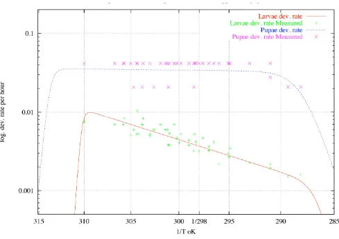
A survey of the literature reveals how very little develop-mental-rate data is available for Anopheles, even for the most important African malaria vectors. The deficit is striking for all of the three major malaria vector species in Africa. We have fit the curve defined by equation 3 to all of the relevant published data. Those data are compiled in tables 1 and 2, for An. gambiae sensus lato.

One reference provided only the total An. gambiae devel-opment time from egg to adult [5], we have then esti-mated the development time for each of the three constituent stages in according with the other data, and also assumed longer development times at low temperatures.

The only gonotrophic cycle data available in relation to temperature was for An. arabiensis, part of the An. gambiae

complex.

All three curves shown in figure 2, for different parameters of equation 2, provide similar fits to the An. gambiae data in tables 1 and 2. These different curves have important implications for vector population dynamics and rein-force the need for more data for these species, particularly at the temperature extremes (low and high), in order to fit an optimal curve. Until there is data for the extreme tem-peratures, any number of curves might fit the data. Three such curves are illustrated in figure 2. For the purposes of this paper the middle of these three curves has been cho-sen, with parameters shown in table 3. The curves for all four stages are shown in figures 3 and 4, with parameters in table 3.

An. gambiae females are one-day old when they take their first blood meal, according to [9]. This greater length of the first gonotrophic cycle has been taken into account [9][10] by defining a coefficient UFirstGon which represents

the time lag before the first blood meal expressed as a percentage of the gonotrophic cycle length. Therefore, the first gonotrophic cycle is considered completed if:

CD(t) >CDf = 1 + UFirstGon + G(0,0.1) (5)

U_FirstGon has been set to 0.5 for An. gambiae. All subsequent gonotrophic cycles follow equation 4.

Thermal mortality

Although the range of variation of water temperature is very wide, it is rarely taken into account in the literature. Some authors have recorded temperatures close to 40°C in small pools [5,11,12]. Such temperatures exceed the thermal death point of many species, including An. funes-tus [5,12]; this may help to explain why these species are

T_t k T_t k r T T exp H R T exp H R T A L ( )= ⋅ ⋅ ∆ ⋅ −            + ∆ ⋅ ° ≠

ρ25 ₂₉₈

1 298 1 1 1 C 1 1 2 1 2

1 1 1

L

H

H

T exp

H

R T T

−                       + ∆ ⋅ −                      

( )2

∆H≠_A

T L 1 2 T H 1 2

CD t_n d_k

Table 1: Published or estimated (*) An. gambiae sensu lato immature stage developmental times (in days). The last point (**) is derived from the Jepson catenary curves.

Temp. °C Egg Larvae Pupae Egg-Adult Species Reference

15.1 2* 25.8* 2* 29.8 SL [27]

16.3 2* 27.2* 2* 31.2 SL [27]

18 1,5* 19.1* 1.5* 22.1 SL [27]

18 1 21.3 1 23.3 ss [28]

20 1 18.4 1 20.4 ss [28]

21.9 1 12 1 14 SL [29]

22 1 15.5 1 17.5 SS [28]

22.1 1 14 1 16 SL [29]

23 1 19 1 21 SL [5]

23.5 1 10 1 12 SL [29]

24 12.9 SS [30]

24 1 11.5 1 12.5 ss [28]

24.6 1 9 1 11 SL [29]

25 1* 13.1* 1* 15.1 SL [27]

25.3 1 10 1 12 SL [5]

25.4 1 8 1 10 SL [29]

25.5 1 13 2 16 SL [5]

25.5 1 8 1 10 SL [29]

26 1 11 1 13 SL [5]

26 1 9.5 1 11.5 SS [28]

26.8 1 8 1 10 SL [29]

27 10.2 SS [30]

27.2 1 9 1 11 SL [29]

27.5 1 6 1 8 SL [29]

Table 2: Published or estimated (*) An. gambiae sensu lato immature stage developmental times (in days). The last point (**) is derived from the Jepson catenary curves (continuing).

Temp. °C Egg Larvae Pupae Egg-Adult Species Reference

28 10.88 SS [31]

28 1 7.8 1 9.8 SS [28]

28.1 1 11 2 14 SL [5]

28.2 1 7 1 9 SL [29]

28.4 1 7 1 9 SL [29]

28.4 1 7 1 9 SL [29]

28.9 1 6 1 8 SL [5]

28.9 1 6 1 8 SL [29]

29.6 1 72 10 SL [5]

30 8.3 SS [30]

30 1 8 1 10 SS [28]

30.7 1 5 1 7 SL [29]

30.8 1 6 2 9 SL [5]

30.8 1* 6.1* 2* 9.1 SL [27]

31.2 7.9 SL [32]

31.3 1 4 1 6 SL [29]

31.4 1 8 1 10 SL [5]

31.7 1 72 10 SL [5]

32 1 8.2 1 10.2 SS [28]

32.7 1 5 1 7 SL [29]

32.8 1 6 1 8 SL [5]

33.7 1 6 1 8 SL [29]

rarely found in small pools. Based on these observations [5,12], a daily mortality in the larval stage of 10%, 50% and 100% for a maximum water temperature of 1, 2 and 3°C above the thermal death point, respectively, has been considered. According to [5] the thermal death point for

An. gambiae is set to 40°C.

Moisture

Anopheles usually develop in natural water bodies, such as puddles, pools or streams [11-14]. The model must take into account two critical parameters in a water body, the temperature and the volume of water. In this stage of the project it was not possible to develop a full water-balance model to estimate those parameters but it should be pos-sible in the future.

Three possible curves fit to An. gambiae larvae development rate data

Figure 2

Three possible curves fit to An. gambiae larvae development rate data.

Table 3: An. gambiae developmental rate parameters.

ρ25°C ∆HL ∆HH

Egg 0.0413 1 -170644 288.8 1000000 313.3

Larvae 0.037 15684 -229902 286.4 822285 310.3

Pupae 0.034 1 -154394 313.8 554707 313.8

Adult 0.02 1000 -75371 293.1 388691 313.4

∆H≠A T1_L 2

T

H

Cloud coverage is likely to be relatively important because of its impact on the water temperature, but this variable is rarely available in climate data. However, it is known that a relative humidity of 100% is usually associated with complete cloud coverage and rain and a relative humidity less than 50% with dryness and almost no clouds. Hence an estimate of cloud coverage as a function of relative humidity RH was made. A clear sky, without clouds (0), for relative humidity below 50%, linearly increases to completely cloudy (1) for relative humidity above 95%, as follows:

The maximum water temperature of a water body depends on the cloud coverage and a user-defined coefficient USunExpo that describes the water body's sun

exposure. This user-defined coefficient represents the coverage or shaded percentage of the particular water body, ranging from 0 for complete shade to 1 for com-plete sunlight exposure. By default it is set to 1.

If the maximum air temperature in degrees Celsius is TM_,

it is estimated that the maximum water temperature in accord with the water volume x (in liters) is

, where:

with C_SE = U_SunExpo·CloudCover(RH). The minimum water temperature is taken as the minimum air temperature. Egg and adult development rates

Figure 3

Egg and adult development rates.

CloudCover RH

RH RH

RH

RH

( )

,

,

,

=

< − _{< <}

< 

 

  

0 50

50

45 50 95

1 95

T_wM

T_wM=TM+ ∆T_xM

∆TxM=

(

)

22 2. ( 1)0 27. 2 (1 ) 0 04. ( 1)0 43. ,10000 ≤≤

− − ⋅ ≥

   

100000

The following formula estimates the daily dynamics of water height W_H in a water body:

where U_IF is the fixed daily water intake in mm·day-1 _(e.g.

from a stream, pipeline, human activity, etc.); its default value is 0. UIV, the variable daily water intake in mm·day

-1_{is set in accord with the precipitation and the}

surround-ing area's topology. Its default value is 1, which would apply to a water body in a flat area, such that only direct rainfall fills the water body. The user can set a particular value: for a water body on a slope, this coefficient should reflect the volume of water intake given 1 ml of precipita-tion in the area. P is the precipitation in mm per day, and

R_H is the relative humidity. U_O, in mm·day-1_{, is the daily}

loss of water due to soil infiltration and evapotranspira-tion. By default, this parameter is set to a mean value of 3

mm·day-1_.

The water bodies are approximated by means of simple geometric objects, such as cubes and cylinders. The default geometric object is a box; its dimensions (length, width, depth) can be entered by the user. Therefore, the volume of water available in the water body is calculated from the particular shape of the water body and the water height calculated above (equation 6).

Larvae and pupae development rates

Figure 4

Larvae and pupae development rates.

WH=WH+UIF+UIV⋅ −P UO−0 1.∗ −(1 ₁₀₀RH)∗USunExpo∗ −(1 CloudCover RH( ))) ( )6

Table 4: Aestivation daily survival.

Daily survival

Egg 0.8

Larvae 0.1

Pupae 0.3

Aestivation and diapause

Unlike the eggs of Aedes aegypti, which, it has been shown, can survive in dry soil for more than two months [6], recent work [15] indicates that Anopheles eggs cannot sur-vive more than 15 days on dry soil. Thus, since some Afri-can regions with endemic malaria experience drought periods longer than two months, the only plausible alter-native seems to be adult aestivation. This is another aspect of Anopheles biology in which much more data is needed. The different survival probability during aestivation has been arbitrarily set as shown in table 4.

Aestivation or diapause is triggered by the non-availability of water (when water bodies are completely dry) for all stages. For the adult stage, aestivation is also triggered by a relative humidity arbitrarily chosen here at less than 40%, though even this may prove to be high in some area.

Nutrient competition

Some combination of regulatory mechanisms limits the size of any population of any species. The most impor-tant, for many species, can be described as density-dependent regulation, or competition for space and/or food, which is assumed to summarize or integrate com-plex, difficult-to-measure mechanisms, such as food mass conversion. For the sake of simplicity and practicality, the basic ecological concept of carrying capacity [16] has been used here. This concept has been applied primarily to the larval stage since it is the longest immature stage and is the only immature stage in which the mosquitoes feed and is, therefore, likely to be the most sensitive to competition. For each water body i a carrying capacity K(i) (in mg) has been defined as:

K(i) = L_Max·S(i)·U_Carrying (7)

where L_Max is the maximum larval biomass density, defined for all species j by:

where N_j is the larval population size per surface unit (m2₎

for species j, and W_j is the approximate mean weight of

species , with and

being the maximum and minimum possible weight in species j, respectively), divided by 2 in equation 8 to cor-rect for the greater size of the low-weight larval popula-tion. LMax = 300 mg·m-2 has been arbitrarily set for larvae.

S(i) is the available water surface in water body i, and U

Car-rying is a positive user-defined coefficient for each water

body, to correct for particular water-body characteristics;

by default it is set to 1. Thus, for each water body at peak season periods, the maximum larval biomass density L_Max

is estimated by measuring the larval population size at its maximum.

Density-dependent mortality

Resource competition is considered as a cause of mos-quito mortality only for the larval stage. For species j [16] the natural increase of the total larval population size, N, (without mortality) can be defined by:

where p is the proportion of larvae that is newly-hatched eggs, estimated by:

where ∆Ne_{(t) is the number of individual eggs entering the}

larval stage.

The carrying capacity K(i) of a particular water body i is defined above (Equation 7). In general, the larval popula-tion increase is given by:

where W(t) is the current larval biomass overall (in con-trast to W_j, the approximate mean weight of species j; see equation 8).

The larval per capita density-dependent mortality rate m

for all species can be approximated by:

Weight

As noted above, the larval stage is the only immature stage with food intake and, therefore, with weight changes. Thus, this stage is the key determinant of the final adult weight.

where

L_Max Nj Wj

j =

∑

( )

Max_j Min_j

( = +

2 WMaxj WMinj

dN t

dt p t N t

( )

( ) ( )

= ⋅

( )

p t N t N t

e

( ) ( )

( )

= ∆

( )

dN t

dt p t N t

K W t K

( )

( ) ( ) ( )

= ⋅ ⋅ −

( )

m t p t W t K

( )= ( )⋅ ( )

( )

C t W W t

K

Food_{i j,} ( ) Max_j

( ) = ⋅ −   

( )

W t W t

j TotalSpecies t

i j i

TotalLarva t j

( ) ( )

# ( )

, # ( , )

and is a coefficient that describes food availa-bility for an individual i of species j, is the maxi-mum possible weight for species j, W(t) is the current larval biomass, K is the carrying capacity of the water body, and W_{i, j}(t) the weight of individual i of species j at time t. For each time step k, for species j, the weight of

individual i increases linearly as

, where d_k is the thermal devel-opment in time period k (equation 2). The weight in the larval stage is then calculated as:

This formula allows the individual larva to have a maxi-mum weight in accord with its species when the larval biomass W << K. At the other extreme the weight increase will be almost zero if W ≈K. Note that this for-mula allows both intra-and inter-species competition for food.

From [5,17-19] the weight parameters for each species have been set as shown in table 5.

For the purpose of stochastic simulation variability has been allowed, again with a default value of 10%, as follows:

W_{i, j} = W_{i, j} + G(0, 0.1) (16)

where G is a normal random variable. The larval stage is regarded as completed, such that the pupa stage begins,

when the thermal development CD is completed (Eq. 4) and Weight >Weight_Min.

The relative weight of an individual within its species is used as an important factor in subsequent subsections on fecundity and number of blood meals, in which the fol-lowing coefficient is used:

Predation and Disease

Predators and pathogens are an important regulating fac-tor and are sometimes reported to be the major cause of mortality [20].

Egg

Little has been reported about An. gambiae egg mortality, from predation or any other cause, beyond an observation (Beier, personal observation) that up to 83% of eggs hatch after one day of drying on sandy loam soil. Without more information, the total egg mortality for each species was arbitrarily set at 5% as a fixed pre-development mortality for the overall batch and a daily survivorship of 0.99. Larvae and Pupae

Service [20] points out that An. gambiae population sizes rise to a peak just after a drought period and then decrease to a roughly stationary level. Life cycles of predators on immature An. gambiae are generally longer than those of their prey, and during the latter phases predators are found in non-predatory stages (i.e. not preying on imma-ture An. gambiae) [20]. Intensity of predation appears to be highly related to the early peak in prey, but there is still a regulatory effect even in the absence of predators. Hence, it is likely that predation is not the only major cause of mosquito mortality [20].

Service [20] evaluated immature An. gambiae sensu lato mortality from predation in two experiments, one in which predator density was high and another in which spraying had reduced predator density. His results are summarized in table 6. With respect to pathogens and parasites, he found that 2.1% to 15.9% of An. gambiae

were infected.

Table 5: Vector weight parameters.

Vector Weight Min (mg) Weight Max (mg)

An. gambiae 0.236 0.383

An. arabiensis 0.33 0.45

An. funestus 0.2 0.33

C_Food t

i j, ( )

W_Max

j

∆W_{i j} t_k =C_Food t_k ⋅d_k

i j

, ( ) _, ( )

W_{i j} t_n W_{i j} t_k

k n

,( )= ∆ , ( ) ( ) =

∑

1

15

W_Max

j

C Weight

Weight

Weight

Max

= ( )17

Table 6: Proportion of death attributable to predation in An. gambiae larvae and pupae.

Stage duration (days) With predators Without predators Attributable to

Predators

Larvae 9.98 90.9 79.58 11.34

Pupae 1.79 73.49 35.63 37.86

Active predation exhibits a lag time around the mean life-cycle length of the prey [20]. During the lag period l, if t =

0 is the start of this period, a curve should show a gradual increase in predation.

The conditions leading to a new predator lag period could occur, for instance, when a dry water body gains water or after a control intervention killing the predators. If (fig. 5):

with and p = 0.001, then the total larval and pupal mortality due to predators and pathogens for spe-cies j, can be expressed as:

Note that ∆mj(t) differs from m(t) in equation 12, which

represents density-dependent mortality. For all species j

the following were arbitrarily set: = 25% for larvae and = 10% for pupae. = 25% is converted to a daily mortality rate as:

where T is the individual's developmental time. Thus at t

= 0, the beginning of the lag period, ∆m_j(t) ≈ 0, and at t ≥ l, for species j.

Predation percentage function of time (lag time)

Figure 5

Predation percentage function of time (lag time).

C t

p

p e p t l

t l

Lag( ) ( ) r t ;

;

= − ⋅ + ≤ ≤ > 

 

 

− ⋅

1 0

1

r l

=11 5.

∆m t_j( )= ∆mmax_j ⋅C_Lag( )t

( )

∆mmax_j

∆mmax_j ∆mmax_j

∆mmax_{j d,} = ∆( mmax T_j )

( )

1

19

On adding to the density-dependent mortality m_j the mor-tality due to predation and pathogens ∆m_j(t), for each spe-cies j, we obtain a new equilibrium K_p <K, given K in equation 11, where

where N_j is the larval population size for species j (N(t) = .

Adult

There are several published studies of adult mortality rates [9,21] for An. gambiae and An. funestus. The causal mechanisms are not clear, but some authors report adult predators preying on adult mosquitoes at oviposition sites [20]. It is assumed that predation-related adult mortality is focused at the water body and that survivorship is greater with fewer predators present.

Oviposition typically occurs every two to three days (see above). Accounting for the low predation during the pre-viously-defined predator lag time, the daily adult survival probability is taken to be 0.911 for a non-ovipositing day and 0.911 - 0.1·C_Lag(t) for An. gambiae sensus lato.

Dispersal

The mechanisms governing mosquito dispersal in general remain unknown. Wind strength and direction are likely to be important factors, for instance, but relevant data are rarely reported. Very little is known about the relative attractiveness of individual humans and individual water bodies to Anopheles, but these cues, along with distance, must be key factors in dispersal.

In most tropical regions, bloodmeals are taken at night, between 6:00 pm and 6:00 am. As the mosquitoes are active during the night, for simplicity bites were modelled only in houses. Bloodmeal source selection is modelled by a two-step process, first a choice of house and second a choice of individual human within the house. Anthro-pophily, the proportion of bites taken on humans, can be set for each Anopheles species overall; the default value of this parameter is 1. Exophily is expressed as the propor-tion of fed mosquitoes that leave the house during the first half of the gonotrophic cycle. For An. gambiae the default value of this parameter is 75%.

The model explicitly, dynamically represents individual locations in space, but at this stage the adult female alter-nately chooses at random among some number of water bodies for an oviposition site, and at random among some number of houses and individuals within the cho-sen house, for a bloodmeal. That is, the choices do not

reflect relative distance, attractiveness, wind or other fea-tures the model is designed to address in future phases of development.

Multiple bloodmeals and multiple bites

In addition to the greater length of the first gonotrophic cycle (Equation 5), Brengues [9] has shown that, to com-plete their first gonotrophic cycle, 42% of female An. gambiae and 63% of female An. funestus require a second bloodmeal one day after the first one. Here the probability of having a second bloodmeal within the first gono-trophic cycle is related to the weight of the individuals: there is a second bloodmeal when the coefficient C_weight is less than 0.4 for An. gambiae.

For multiparous females, there is a second bloodmeal when C_weight is less than 0.1.

According to [22], 14% of female An. funestus and 19% of female An. gambiae that had just fed had taken only a par-tial bloodmeal. These figures are used to represent the proportion of females that take a subsequent bite within what is considered the same bloodmeal.

Fecundity

The number of eggs oviposited by individuals shows a wide range of variation, both within and between experi-ments [17,18,23,24]. The mean number of eggs ovipos-ited is defined by m = 100, with a standard deviation s = 50. In the absence of more precise information these val-ues are assumed. The number of eggs oviposited is simu-lated as:

N = G(m, s)·U_Egg (21)

where U_Egg is a positive user-defined coefficient set to fit local observations, by default set to 1, and G is a normal random variable. Because fecundity is closely tied to body size, a variability of 50% of the number of eggs is allowed as a function of the individual's weight, as follows (see [18][23]):

N' = N·(0.5 + 0.5·C_weight) (22)

The male-female ratio at emergence from the pupa stage is assumed to be 1:1.

Results

A simple example is used to show how the model can help to achieve a better understanding of vector population dynamics and determine key underlying factors. In partic-ular, the influence of temperature, moisture, predation and nutrient competition on adult abundance is investi-gated. The example is taken as a small cluster of six houses, each with five residents, and a total of three

K t K

p t m t N t

p N t

p j j j ( ) ( ( ) ( )) ( ) ( ) ( ) = ⋅ − ∆ ⋅ ⋅

∑

N t_j

j ( ))

oviposition sites (figure 6 and table 7. An attempt has been made to reproduce some important characteristics of a local environment by considering two types of pools: a semi-permanent pool, P1, and two temporary pools, P2 and P3 (see figure 7 and table 7. As noted above, at this stage each mosquito in the model chooses at random among oviposition sites and among houses and residents at the appropriate points in her gonotrophic cycle. Tem-perature and moisture inputs were obtained based on data from Kilifi, on the coast of Kenya. Figures 8 and 9 show daily precipitation, minimum and maximum tem-perature and relative humidity reported there over the 20 months from May 1, 2000 to December 31, 2001. In this region there are two primary rainy seasons: April-June and October-November. Except where noted, the default val-ues were used for parameters, as given above.

Effects of temperature

In the first set of simulations there are 300 eggs and 10 adults, with all six houses but only pool P1 present. Figure 10 shows the variability and mean of twenty replicates realizations of the simulation model, an effect of the sto-chasticity allowed in the cumulative development time (equation 4), length of initial gonotrophic cycle (equa-tion 5) and number of eggs oviposited (equa(equa-tion 21). The abundance curve is predicted from the preceding environ-mental data, with each run started on May 1, 2000. This

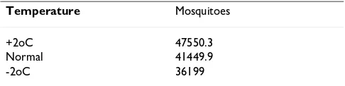
An. gambiae adult mean curve shows similarities to several published curves, at much wider scales [25], in that there are relatively low levels of mosquitoes throughout the year, with fluctuations in abundance that may correspond to the limitations of competition and/or predation and several very high peaks in short time intervals. To analyse the effects of temperature, two additional temperature curves were used, one in which the actual temperatures are increased by two degrees and one in which they are low-ered by two degrees Celsius, the results are shown in figure 11. Table 8 shows the impact of temperature on adult abundance. For An. gambiae (figure 11), with increasing temperature there is a general increase in the level and number of peaks. As detailed above in the section on Temperature (table 1 et seq.), the egg-to-adult develop-ment time is shortened with higher temperature, thus pro-ducing more mosquitoes. The two-degree temperature

rise increases An. gambiae adult abundance over the full 19 months by 15%; the two-degree temperature drop decreases it by 17% overall. Recall that multiple factors interact to determine the adult abundance at each point; however, predation is probably not a critical biotic regu-lating factor by the time of the initial peak, for instance, but nutrient competition/carrying capacity probably can have a strong impact at late stages of this initial peak. In general, although the drought period from March 12, 2001 to March 31, 2001 has the effect of allowing a first big peak in adult abundance for An. gambiae, it also synchronizes the first peak, and might be important for control intervention purposes.

The overall pattern of adult abundance appears well-con-served, and the variability relatively minor.

However, as noted above, the aim here is simply to sug-gest the potential of the model. Figure 10 shows the stand-ard deviation (variability) of the twenty replicate for each date.

Effects of temporary pools

Here An. gambiae is considered and examined for the effect on adult abundance of adding pools P2 and P3 to the semi-permanent pool P1, beginning with 10 adults and 300 eggs in each pool. Pools P2 and P3 may be clas-sified as temporary, since they dry two or three times dur-ing the year (see figure 7). Beside the expected increase in the total number, there is a much more dramatic fluctua-tion in the mosquito abundance curve, with six added major peaks (figure 12).

Effects of interventions

Here An. gambiae is considered, with pool P1 only, and show how the model might be of help in reducing peaks in adult abundance by helping to optimize the control of larval and adult populations. Recall that the goal here is not to allege or prove a particular finding, which can depend on a specific environmental situation, but to show how the model could help address a given question in a specific environmental situation, and help in under-standing the mechanisms involved. The aim is to show

Table 7: Water body characteristics

sun exposure coef water fill water fix intake (mm) water fix lost (mm) max biomass density (mg·m-2₎

Pool 1 1 4 0 0.01 30

Pool 2 1 7 0 0.02 60

examples, with graphical representation, of how such a model can be a powerful tool in research on malaria vector dynamics. For the purpose of the first analysis the predator population is excluded from any effects of the larval control intervention. Therefore, the impact of the predator as described above (in the Predation section) will remain constant.

Although the focus is the first major peak in adult abun-dance, the analysis could be transposed to any period. Interventions that take effect in two periods are compared, the first beginning on May 6, 2000, at the beginning of the first major peak, and the second beginning 15 days later, on May 21, 2000. A successful one-time larval control intervention is simulated by imposing 80% mortality on all larvae present during 10 consecutive days. An adult control intervention that consists of spraying surfaces inside houses with residual insecticide is simulated by imposing 75% mortality on blood feeding adults during a 25-day period.

Figure 13 indicates that the later larval-control interven-tion (5/21/00), though done at the highest adult abundance rates, would have almost no effect on overall adult abundance, since it happens at a period of lower lar-val abundance. Still worse, it could lead to the production of bigger mosquitoes by diminishing the nutrient compe-tition. On the other hand, a larval-control intervention that began only 15 days earlier would nearly eliminate the entire first peak in adult abundance. This emphasizes the need of good forecasting tools.

Similarly, for an adult-control effort (figure 14), the later control intervention would have very little impact, but the first peak in adult abundance could be decreased conse-quently by an effort that began only 15 days earlier. At this stage the model does not take into account such impor-tant factors as insecticide resistance and mosquito avoid-ance behavior, which would tend to diminish the impact of spray programs. A combined control intervention (fig-ure 15) shows similar patterns and suggests that the single most effective intervention approach would be an early focus on larval control.

Effects of interventions on predators

In this analysis the same conditions are considered as the preceding section but the potential impact of the control interventions on predators is also taken into account. In the case of the larval control intervention, 80% mortality in the predator population is assumed, as was observed by [20]. The predator pressure returns to its normal level after a time lag of 21 days (see Predator section).

To the best of our knowledge, no study has focused on predators on adult Anopheles within houses, but spiders in

particular are thought to be very efficient in preying on mosquitoes. Here the impact of the destruction of these predators is investigated under an assumption that they represent an adult mosquito mortality of 5%. It is also assumed that the predator-pressure returns to its normal level after a time lag of 21 days.

Figures 16, 17 and 18 show the impact of predators on the vector population.

Figure 16 shows that the removal of predators has a big impact on the effect of a larval control intervention: the first peak is much less flattened, as it was in the previous section, and is displaced by about seven days.

The lack of predator pressure allows a much quicker reconstruction of the larval population.

For the adult control intervention, the curves in figure 17 show almost no differences. However, the half-life of the adult mosquito population increases by one day (from 4.6 to 5.7 days), which is of great epidemiological interest since this would increase the vectorial capacity by allow-ing more mosquitoes to become infectious.

Figure 18 considers the effects of a combined larval and adult control intervention for 10 and 25 days respectively and makes several points. First, the combined control intervention seems to have a stronger impact in terms of reducing the adult population. However, it was noted that the peak in adult abundance (with the predator simulation) is higher than the one without the predator simulation and also that there is a dramatic three-day increase in adult half-life (from 4.6 to 7.5 days). Further-more, if the larval control intervention is delayed by 20 days, the consequences include not only the persistence of Example schematic

Figure 6

a fairly high first peak but also a higher second one. There-fore, such a model could be very important in helping to assess the optimal timing for vector control interventions.

Discussion

This model integrates important mechanisms underlying

Anopheles population dynamics in an explicit, transparent

way. It focuses on five basic factors, two of them abiotic – temperature and moisture – and three biotic – nutrient competition, predation or death by disease, and dispersal. Little of the published literature takes into account the effects of temperature on vector populations. It may be that temperature shows little fluctuation compared to Water height in pools

Figure 7

Water height in pools.

Rainfall and Temperature

Figure 8

countries with marked seasonality, but most African regions like Kenya exhibit temperature fluctuations

rang-ing from 16°C to 35°C, which can be critical. Futher-more, temperature range is a key determinant for species dispersal and is, therefore, of high epidemiological importance: the species have different vectorial capacities and require different control programs.

Each parameter in equation 2 is individually related to the slopes of the curves for each stage of insect development (see Schoofield et al. [8]), and therefore may reflect a spe-cies' adaptation to different climates. Particularly, , Relative humidity

Figure 9

Relative humidity

Simulated An. gambiae adult abundance at actual temperatures for 20 simulations

Figure 10

Simulated An. gambiae adult abundance at actual temperatures for 20 simulations

Table 8: Impact of temperature on adult abundance.

Temperature Mosquitoes

+2oC 47550.3

Normal 41449.9

-2oC 36199

An. gambiae adult abundance, mean of 20 simulations for each temperature level

Figure 11

An. gambiae adult abundance, mean of 20 simulations for each temperature level

An. gambiae adult abundance with all three pools (P1, P2 and P3) mean of 20 simulations

Figure 12

An. gambiae adult abundance with all three pools (P1, P2 and P3) mean of 20 simulations

An. gambiae adult abundance with larval control intervention

Figure 13

An. gambiae adult abundance with adult control intervention

Figure 14

An. gambiae adult abundance with adult control intervention

An. gambiae adult abundance with larval and adult control intervention

Figure 15

An. gambiae adult abundance with larval and adult control intervention

An. gambiae adult abundance with larval control intervention and predators

Figure 16

∆H_H and ∆H_L, should reflect the sensitivity of each species to temperature changes in temperate, high and low tem-perature areas respectively, and thus could be highly informative. Many studies focus on vector breeding site characteristics, which the model addresses simply in terms of moisture. As yet no particular variables have been

found to be crucial determinants of breeding site selection or success, but when these are determined, the model can implement them relatively easily. The transient patterns of breeding sites are taken into account as key determinants of predator and vector disease dynamics, however. An. gambiae adult abundance with adult control intervention and predators

Figure 17

An. gambiae adult abundance with adult control intervention and predators

An. gambiae adult abundance with larval and adult control intervention and predators

Figure 18

Nutrient competition is considered one of the major reg-ulators of vector populations. Here the carrying capacity concept is used to allow both intra-and inter-species competition. Very few studies of vector predators and pathogens have been undertaken to date, but some litera-ture suggests that this may also be an important determi-nant, so it has been incorporated accordingly. Little is known about Anopheles dispersal, though this is clearly a critical factor. Here simple random dispersal has been used, but it may be possible to implement a more sophis-ticated dispersal algorithm soon.

Thus, a basic tool has been developed for use by field workers and will be vastly improved by their efforts. First, more complete and precise data on Anopheles biology is needed: if nothing else, the model provides an organized view of the huge gaps in the existing information. A framework has been developed by exploiting what is available, but, at this point, far too many parameters and mechanisms involve arbitrary values or estimates. Nonetheless, as an example, a vector population was sim-ulated for a 20-month period, from May 1, 2000 to December 31, 2001, with meteorological data from Kilifi in Kenya and it was possible to roughly assess the sensitiv-ity of vector population dynamics to four of the five basic factors – temperature, moisture, competition, and preda-tion. The focus was on adult abundance curves.

Temperature is very important to the adult abundance curve and, particularly, to the occurrence of the initial peak after a drought period; this may be critical for control purposes. Moisture is a key determinant of particular high peaks that occur not only after a drought period but throughout the year for temporary breeding sites. These peaks were attributed to the lower larval mortality pro-ceeding from lower predation and disease pressure. These peaks may be of great epidemiological importance, in that they could bring malaria prevalence in humans above a threshold at which relatively high transmission could occur despite a low vector density. One concern with such large fluctuations is that the proportion of peo-ple susceptible may be very high at the beginning of the peak period. Furthermore, the earliest emergent adult mosquitoes may have a higher vectorial capacity; with almost no food competition, their weight is greater, which implies a longer life [26]. With different initial conditions, when high density competition induces longer development time, the occurrence of the first peak can be delayed by more than a week.

Preliminary results on species competition suggest the existence of competitive exclusion, i.e. the survival of only one species in a given habitat, which highlights the

neces-sity of niche differentiation for species coexistence. The example also suggests that if insecticides impact popula-tions of predators on Anopheles, the resulting de-regula-tion may backfire, producing a vicious cycle that leads to ever-increasing insecticide use. This further supports the argument that great improvements in our understanding of Anopheles ecology and population dynamics are needed.

The model is based on the data and knowledge currently available, and it can reproduce some broad, diverse pat-terns found in the field; its mechanisms and rules are explicit, and they allow us to provide detailed analyses and explanations of vector population dynamics. How-ever, it requires considerable, continued application in the field to improve the data and our understanding of the underlying mechanisms. This is exactly the plan for subse-quent research, to contribute to improved control of the scourge of malaria.

Table 9 shows the parameters in the most immediate need of field testing and measurement. However, with the default parameter setting, the model can currently be run by users with only:

1. A description of the geographical area with the pools and houses.

2. Climate information (temperature, precipitation, rela-tive humidity) for the period considered.

Conclusions

This model made it possible to structure existing knowl-edge of Anopheles vector population dynamics, and high-light crucial elements that are missing.

The data and other information currently available made it possible to build a model that can reproduce diverse patterns found in the field. It incorporates explicit mecha-nisms and rules that can provide detailed analyses and explanations, and thus is a tool to help the malaria

Table 9: Parameters to define.

Daily survival

Egg aestivation survival Adult aestivation survival

Adult aestivation trigger (relative humidity level/ factors combination) Maximum larval biomass per surface unit

research and intervention community gain a better under-standing of vector dynamics.

The model should be greatly improved as more precise data and hypotheses become available and as it is applied in the field.

Authors contributions

• JMD contributed conceptualisation and design of the model, main literature review and authorship of the paper.

• CM contributed conceptual and data input, review and comments.

• GK, BK, JB and JC contributed conceptual input, review and comments.

• JD, PB, HM, JG and AT contributed review and comments.

• FEM contributed the initial concept and general supervision.

All authors read and approved the manuscript.

Acknowledgements

We wish to thank Lizette Koekemoer of the South African Institute of Medical Research for a advice and provision of unpublished data.

References

1. Sherman IW: Malaria Washington DC: American Society for Microbi-ology (ASM) Press; 1998.

2. Hii J, Smith T, Vounatsou P, Alexander N, Mai A, Ibam E, Alpers M:

Area efects of bednet use in malaria-endemic area in Papua New Guinea.Trans R Soc Trop Med Hyg 2001, 95:7-13.

3. Wernsdorfer WH, McGregor SI: Malaria, Principles and Practice of MalariologyVolume 2. Edinburgh: Churchill Livingstone; 1988. 4. Hay SI, Myers MF, Burke DS, Vaughn DW, Endy T, Ananda N, Shanks

GD, Snow RW, Rogers DJ: Etiology of interepidemic periods of mosquito-borne disease. Proc Natl Acad Sci USA 2000,

97:9335-9339.

5. Jepson WF, Moutia A, Courtois C: The malaria problem in Mau-ritius: The bionomics of Mauritian anophelines.Bull Entomol Res 1947, 38:177-208.

6. Focks DA, Haile DG, Daniels E, Mount GA: Dynamic life table model for Aedes aegypti (Diptera: Culicidae): Analysis of the literature and model development. J Med Entomol 1993,

30:1003-1017.

7. Sharpe P, DW D: Reaction kinetics of poïkilotherm development.J Theor Biol 1977, 64:649-670.

8. Schoolfield R, PJH S, CE M: Non-linear regression of biological temperature-dependant rate models based on absolute reaction-rate theory.J Theor Biol 1981, 88:719-731.

9. Brengues J, Coz J: Quelques aspects fondamentaux de la biolo-gie d'Anopheles Gambiae Giles (Sp An.) et d'Anopheles Funes-tus Giles en zone de savane humide d'Afrique de 1'Ouest.Cah ORSTOM Sér Ent et Parasitol 1973, XI(2):107-126.

10. Gillies MT: The duration of the gonotrophic cycle in Anopheles Gambiae and Anopheles Funestus, with a note on the effi-ciency of hand catching.East Afr Med J 1953, 30:129-135. 11. Minakawa N, Mutero CM, Githure JI, Beier J, Yan G: Spatial

distri-bution and habitat characterization of anopheline mosquito larvae in western Kenya.Am J Trop Med Hyg 1999, 61:1010-1016.

12. De Meillon B: Observations on Anopheles funestus and Anoph-eles gambiae in the Transvaal. Publ S Afr Inst Med Res 1934,

6:195-248.

13. Gimnig JE, Ombok M, Kamau L, Hawley WA: Characteristics of Larval Anopheline (Diptera: Culicidae) Habitats in Western Kenya.J Med Entomol 2001, 38:282-288.

14. Minakawa N, Seda P, Yan G: Influence of host and larval habitat distribution on the abundance of African malaria vectors in western Kenya.Am J Trop Med Hyg 2002, 67:32-38.

15. Koenraadt CJ, Paaijmans KP, Githeko AK, Knols BG, Takken W: Egg hatching, larval movement and larval survival of the malaria vector Anopheles gambiae in dessicating habitats.Malar J 2003,

2:20.

16. Begon M, Harper JL, Townsend CR: Ecology, Individuals, Populations and Communities Oxford: Blacwell Science Ltd; 1996.

17. Takken W, Klowden MJ, Chambers GM: Effect of body size on host seeking and blood meal utilization in Anopheles gambiae sensu stricto (Diptera: Culicidae): the disadvantage of being small.J Med Entomol 1998, 35:639-645.

18. Lyimo EO, Takken W: Effect of body size on fecundity and pre gravid rate of Anopheles gambiae females in Tanzania.Med Vet Entomol 1993, 7:328-332.

19. Koella JC, Lyimo EO: Variability in the relationship between weight and wing length of Anopheles gambiae (Diptera: Culicidae).J Med Entomol 1996, 33:261-264.

20. Service MW: Mortalities of the immature stages of species B of the Anopheles gambiae complex in Kenya: Comparison between rice fields and temporary pools, identification of predators, and effects of insecticidal spraying.J Med Entomd 1977, 13:535-545.

21. Clements A, Paterson GD: The analysis of mortality and survival rates in wild populations of mosquitoes. J Appl Ecol 1981,

18:373-399.

22. Charlwood J, Smith T, Kihonda J, Heiz B, Billingsley P, Takken W:

Density independent feeding success of malaria vectors (Diptera: Culicidae) in Tanzania. Bull Entomol Res 1995,

85:29-35.

23. Hogg JC, Thompson MC, Hurd H: Comparative fecundity and associated factors for two sibling species of the Anopheles gambiae complex occuring sympatrically in the gambia.Med Vet Entomol 1996, 10:385-391.

24. Maharaj R: Effects of temperature and humidity on adults of the Anopheles Gambiae complex (Diptera: Culicidae) in South Africa – implications for malaria transmission and control.PhD thesis. University of Natal 1995.

25. Patz JA, Strzepek K, Lele S, Hedden M, Greene S, Noden B, Hay SI, Kalkstein L, Beier J: Predicting key malaria transmission fac-tors, biting and entomological inoculation rates, using mod-elled soil moisture in Kenya.Trop Med Int Health 1998, 3:818-827. 26. Ameneshewa B, Service MW: The relationship between female body size and survival rate of the malaria vector Anopheles arabiensis in Ethiopia.Med Vet Entomol 1996, 10:170-172. 27. Le Sueur D: The ecology, over-wintering and population

dynamics of the pre-imaginal stages of the Anopheles Gam-biae Giles complex (Diptera culicidae) in northern natal, South Africa.PhD thesis, University of Natal, South Africa 1991. 28. MN B, SW L: Effect of temperature on the development of the

aquatic stages of Anopheles gambiae sensu stricto (Diptera: Culicidae).Bull Entomol Res 2003, 93:375-381.

29. Holstein MH: Biology of Anopheles gambiae : research in French West Africa.Tech rep., World Health Organization, Palais des Nations, Geneva 1954. Monograph Series No9

30. Lyimo EO, Takken W, Koella J: Effect of rearing temperature and larval density on larval survival, age at pupation and adult size of Anopheles gambiae. Entomol Exp Appl 1992,

63:265-271.

31. Schneider P, Takken W, McCall PJ: Interspecific competition between sibling species larvae of Anopheles Arabiensis and An. Gambiae.Med Vet Entomol 2000, 14:165-170.

32. Gimnig JE, Ombok M, Otieno S, Kaufman MG, Vulule JM, Walker ED:

Density-dependent development of Anopheles gambiae (Dip-tera: Culicidae) larvae in artificial habitats.J Med Entomol 2002,