Importance of factors determining the effective lifetime of a mass, long lasting, insecticidal net distribution: a sensitivity analysis

R E S E A R C H

Open Access

Importance of factors determining the effective

lifetime of a mass, long-lasting, insecticidal net

distribution: a sensitivity analysis

Olivier JT Briët

, Diggory Hardy

and Thomas A Smith

Abstract

Background:Long-lasting insecticidal nets (LLINs) reduce malaria transmission by protecting individuals from infectious bites, and by reducing mosquito survival. In recent years, millions of LLINs have been distributed across sub-Saharan Africa (SSA). Over time, LLINs decay physically and chemically and are destroyed, making repeated interventions necessary to prevent a resurgence of malaria. Because its effects on transmission are important (more so than the effects of individual protection), estimates of the lifetime of mass distribution rounds should be based on the effective length of epidemiological protection.

Methods:Simulation models, parameterised using available field data, were used to analyse how the distribution’s effective lifetime depends on the transmission setting and on LLIN characteristics. Factors considered were the pre-intervention transmission level, initial coverage, net attrition, and both physical and chemical decay. An ensemble of 14 stochastic individual-based model variants for malaria in humans was used, combined with a deterministic model for malaria in mosquitoes.

Results:The effective lifetime was most sensitive to the pre-intervention transmission level, with a lifetime of almost 10 years at an entomological inoculation rate of two infectious bites per adult per annum (ibpapa), but of little more than 2 years at 256 ibpapa. The LLIN attrition rate and the insecticide decay rate were the next most important parameters. The lifetime was surprisingly insensitive to physical decay parameters, but this could change as physical integrity gains importance with the emergence and spread of pyrethroid resistance.

Conclusions:The strong dependency of the effective lifetime on the pre-intervention transmission level indicated that the required distribution frequency may vary more with the local entomological situation than with LLIN quality or the characteristics of the distribution system. This highlights the need for malaria monitoring both before and during intervention programmes, particularly since there are likely to be strong variations between years and over short distances. The majority of SSA’s population falls into exposure categories where the lifetime is relatively long, but because exposure estimates are highly uncertain, it is necessary to consider subsequent interventions before the end of the expected effective lifetime based on an imprecise transmission measure.

Keywords:LLIN, Simulation, Life, Mass, Distribution, Lasting, Insecticidal, Net

Background

Over the period 2008-2010, an estimated 290 million long-lasting insecticidal nets (LLINs) were distributed in sub-Saharan Africa [1]. LLINs reduce malaria transmis-sion by protecting individuals from infectious bites, and

by reducing the probability that a mosquito survives the extrinsic incubation period. Whereas continuous distri-bution through antenatal clinics is common, most LLINs are being distributed through mass campaigns, reaching a large proportion of the population at risk of malaria. Over time, after a mass distribution, the pro-portion of the population sleeping under an LLIN decreases. This is partly due to attrition (the loss of nets available for their intended use, e.g. by alternative use), * Correspondence: [email protected]

1

Department of Epidemiology and Public Health, Swiss Tropical and Public Health Institute, Basel, Switzerland

Full list of author information is available at the end of the article

but also due to new births and user fatigue adding to the unprotected population.

The effective protection of LLINs against mosquito bites also wanes as they decay physically (hole forma-tion) and chemically (insecticide loss).

Many LLIN programmes work with the assumptions that there is little variability in the decay among nets and that they last about 3 years, at which time they need replacement. However, variability in net decay appears to be substantial and the average‘lifespan’could be considerably less than 3 years [2]. The number of LLINs remaining in households does not take the physi-cal and chemiphysi-cal state of the nets into account, and a proportion of those nets may have lost considerable functionality [3]. The World Health Organization (WHO) recommends tracking the physical integrity of nets (number, size and location of holes) and the insec-ticidal activity, measured by knock down and killing in standard WHO cone and tunnel tests [2]. Unfortunately, little is known about how these quantities, alone or in interaction, affect personal protection, and how they could be used to define when a net is worn out and at the end of its‘useful life’.

Even if individual nets do not adequately prevent mos-quitoes from inoculating the user, they may still reduce mosquito survival and thus affect transmission at the population level. This community effect is likely to be more important than personal protection in preventing inoculations [4,5]. The timing of repeat LLIN distribu-tions may also depend on the characteristics of the human population, in particular the transmission level and immune status. Whereas knowing the‘useful life’of individual LLINs (for which a cut-off minimum func-tionality would need to be defined, below which an LLIN would be declared‘dead’) might facilitate planning in continuous distribution programmes. For a round of mass distributed LLINs, the ‘effective lifetime’, based on the duration of the malaria preventive effect at popula-tion level capturing all the effects described above, might be more useful for planning the timing of subse-quent rounds.

This paper describes a simulation experiment to pre-dict the duration of epidemiological protection offered by a mass LLIN distribution targeting the general popu-lation and identifies the factors that are important in determining it.

Methods

The OpenMalaria modelling platform [6] is an open source C++ programme and takes scenario specification inputs in eXtensible Markup Language (XML). In this platform, stochastic individual-based models for malaria in humans are combined with a deterministic model for malaria in mosquitoes, which have been fitted to

multiple field data sets [7]. For each five-day time step, data on a human population is updated via components representing new infections, parasite densities, acquired immunity, uncomplicated and severe malaria episodes, direct and indirect mortality, infectiousness to mosqui-toes, and case management. Each simulated malaria infection has a distinct parasite density that varies by time step, while the malaria transmission level varies seasonally. The models can accommodate multiple mos-quito species with varying periodical emergence rates, and non-human hosts [8,9]. An ensemble of 14 model variants [10] is currently available, capturing a range of possibilities for the dynamics of malaria in humans.

For this experiment, the existing insecticide treated net (ITN) intervention model component [8,9] was developed to include capability to model physical and chemical decay of LLINs. The effect of LLINs, depend-ing on their physical and chemical state, on deterrence, pre-prandial and post-prandial killing of malaria vector mosquitoes (see Appendix) was parameterised, using published experimental hut data [11-14].

Outcomes based on the incidence of all-age uncompli-cated and clinical malaria episodes were considered, which is the measure of the malaria burden most easily accessible in control programmes. Full economic analy-sis should weight severe and fatal episodes more heavily and take age into account, but in these models there is considerable uncertainty about predicted morbidity rates in older age groups. The following measure of effective lifetime was used: the length of the period since mass distribution during which the number of prevented epi-sodes was above half the numerical value of the year with maximum impact on malaria episodes (i.e. the year with the minimum number of malaria episodes), as compared to a scenario without any intervention. A sen-sitivity analysis was done on how the effective lifetime of a mass LLIN distribution depended on the pre-interven-tion entomological inoculapre-interven-tion rate (EIR) (which was varied by scaling vector emergence), initial coverage, attrition rate, LLIN effects, and physical and chemical decay rates and other LLIN-related parameters. Each of 14 parameters or parameter groups (listed in Figure 1 and discussed in the Appendix) were varied over three values (low, central and high), while keeping all other parameters and parameter groups at their central values (see Additional file 1 and the link [15] for an interven-tion scenario with all parameters at central value).

Also, selected parameter and parameter group combi-nations that seemed likely to be interdependent or to have multiplicative effects (Figure 1), were varied. For each combination, parameter values were chosen that acted on the outcome in the same direction. This was done both with those parameter values in the combina-tion associated with lower outcomes, and with those

Briëtet al.Malaria Journal2012,11:20 http://www.malariajournal.com/content/11/1/20

values associated with higher outcomes. The parameters outside the combinations were kept at central values.

The relationship between the effective lifetime and pre-intervention EIR was studied in more detail by vary-ing it over a wider range, together with LLIN attrition half-life. The effect of initial coverage was also looked at in more detail. Because the cut-off at half the impact on malaria episodes in the definition of the effective life-time is arbitrary, sensitivity to this was studied. Finally, whether or not the protective epidemiological impact could be sustained in hypothetical situations where cov-erage is sustained throughout and where nets do not decay, depending on the pre-intervention EIR and cov-erage, was explored.

Results

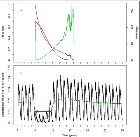
Figure 2 illustrates a simulation run of the central sce-nario with the base model (R0000). At the beginning of the sixth year of the simulation, LLINs were assigned to 70% of the population. Over time, the coverage declined, the insecticide in the remaining LLINs declined, and the hole index in the remaining LLINs increased (Figure 2a). Because of variation in the rates of insecticide loss and hole formation, the curves for the mean hole index and mean insecticide content became erratic as fewer LLINs remained. In the absence of intervention, the

number of episodes per person per five-day time step (Figure 2b) reflects the annual periodicity of the vector emergence. The effect of an LLIN distribution is best illustrated by the de-seasonalised trend. Immediately after LLIN assignment, the number of episodes declined, reaching a minimum after two years. The number then rose with an S-shaped curve, reaching a slightly higher level than pre-intervention, and declined gradually to the pre-intervention level. The red arrow in Figure 2b illustrates the approximate point where the impact of the LLIN distribution round is half of its maximum, and the time from distribution until that point.

The results of the sensitivity analysis are plotted in a ‘skeleton’diagram (Figure 1), which is an adaptation and expansion of a tornado diagram. A skeleton diagram not only displays how strongly the outcome varies with each parameter over its tested range, with all other para-meters at their central values; it also indicates, for selected parameter combinations only, how the sensitiv-ity to a parameter is altered if other parameters on which the parameter in question might be contingent are at their extremes.

Effective lifetime appears to be particularly sensitive to three parameters: pre-intervention EIR (annualEIR), attrition of nets (attritionOfNets half-life) and half-life of insecticide decay (insecticideDecay L).

The skeleton diagram shows that, for example, the bar lengths forcoverage,deterrency,preprandialKillingEffect, andpostprandrialKillingEffectare shorter for the centre-to-low (red) bars connected to the lower extreme for attri-tionOfNets half-life(red cross), than for those connected to the central level ofattritionOfNets half-life(blue cross).

Because the attrition rate determines in part how many nets are left (together with the initial receipt

proportion, defined by the parameter coverage), it strongly interacts with parameters that describe the LLIN effects on the vector population. At the lower extremes of both attritionOfNets half-lifeand prepran-dialKillingEffect, the centre-to-low (red) bar for the insecticideScalingFactor is only slightly shorter than the centre-to-low (red) bar with bothattritionOfNets half-life and preprandialKillingEffect (and all other

Figure 2Central scenario simulation with base model. a) The blue line (on left vertical axis) represents the proportion of the population covered, the red line (on left vertical axis) represents the mean insecticide in the remaining LLINs as a proportion of its initial value. The light green line (on the right vertical axis) represents the mean hole index in the remaining LLINs. b) The black line represents the number of episodes per person per five-day period. The dark green line represents the 1 year moving average of the number of episodes per person per five-day period. The red arrow indicates the approximate length of the effective lifetime of the LLIN distribution.

Briëtet al.Malaria Journal2012,11:20 http://www.malariajournal.com/content/11/1/20

parameters) at central level. Further, one level deeper, at the lower extreme of the insecticideScalingFactor, the length of the centre-to-low (red) bar forinsecticideDecay Lis shorter than that with all other parameters at cen-tral level, yet still important. From Figure 1, it is not possible to establish how much the variation in each of the parameters for attritionOfNets half-life, prepran-dialKillingEffect, andinsecticideScalingFactorcontributes to the shortening of the insecticideDecay L bar. How-ever, it is likely that attritionOfNets half-life has an important role, as insecticide decay only acts on remain-ing nets and is thus strongly contremain-ingent on the attrition rate. At a long attrition half-life, the sensitivity to the mean insecticide decay rate and its‘downstream’ para-meter (the parapara-meter for variation in insecticide decay is contingent on the mean insecticide decay rate) will be much stronger than at a shorter attrition half-life because most nets will disappear in the latter scenario before the decay rate matters much. This is similar for the mean hole formation rate and its‘downstream’ para-meters (the parapara-meters for variation in the hole forma-tion rate and the rip factor are contingent on the mean hole formation rate). TheholeRate meanis more impor-tant at the higher extreme ofattritionOfNets half-life, preprandialKillingEffect, andholeScalingFactorthan with all parameters at central level. Nevertheless, the out-come appears to be insensitive to parameters determin-ing physical decay (hole formation).

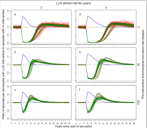
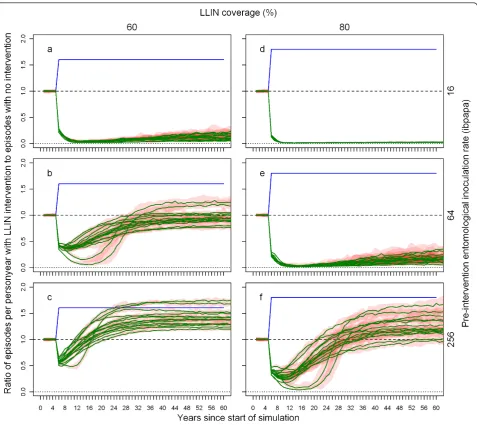
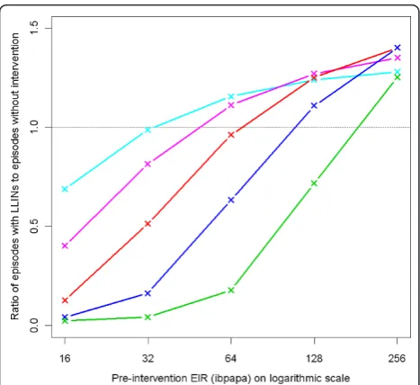
Figure 3 illustrates how, depending on the pre-inter-vention EIR and attrition half-life, the ratio of malaria episodes per year for a situation with LLINs to a situa-tion without LLINs develops over time. In general, the number of episodes reaches a minimum a few years after distribution that is slightly lower than in the first year after distribution, and then increases with an S-shape, becoming larger than one (indicating more epi-sodes in the intervention situation) before gradually dropping to one. With increasing pre-intervention EIR, the minima are not as low, the subsequent rise in epi-sodes less steep, and the maxima are higher. With a lower attrition rate (longer half-life of 5 years) the graphs appear to be horizontally stretched versions of the situation with higher attrition (shorter half-life of 3 years). At a low pre-intervention EIR, the impact on malaria episodes lasts until most LLINs have disap-peared. At a high pre-intervention EIR, there are still a large number of nets (albeit with holes and less insecti-cide) present when the number of episodes surpasses the pre-intervention level. At higher pre-intervention EIRs, the simulation run ranges are very narrow, indicat-ing that there is little stochasticity (and that a popula-tion size of 10,000 is appropriate). Particularly for the lower pre-intervention EIRs, three model variants, R0063, R0065 andR0068, which vary heterogeneity in

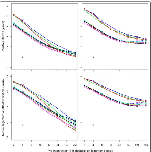
human exposure [10], yield results that are different from the 11 other variants, with longer lasting LLIN effects. This is illustrated by Figure 4, which shows how the effective lifetime outcome depends on pre-interven-tion EIR and model variant, at an attripre-interven-tion half-life of four years. If effective lifetime is defined based on the incidence of infections (Figure 4c &4d) instead of epi-sodes (Figure 4a &4b), then lifetime is consistently higher for these model variants than for the base model. For episodes, however, the effective lifetime with model R0068converged with that of the base modelR0000at high pre-intervention EIR levels, and the lifetime of modelsR0063 andR0065 decreased more sharply with increasing pre-intervention EIR than with the base modelR0000.

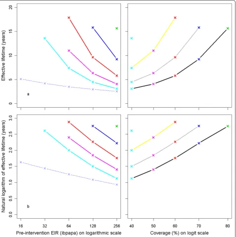
Effective lifetime, averaged over all 14 model variants, is plotted against the pre-intervention EIR in Figure 5a. The relationship follows approximately a straight line if the outcome is logarithmically transformed (Figure 5b). The effective lifetime is linearly related to the logarithm of the attrition half-life (Figures 5c and 5d).

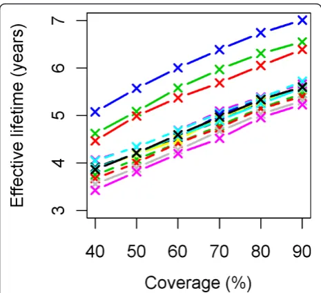
Figure 6 illustrates how effective lifetime depends on initial coverage. This appears to be a linear relationship with the proportion of the population having access to an LLIN. As the lines for model variants are largely par-allel to one another, there is little interaction between model specification and initial coverage over the range studied.

The sensitivity of the result to the definition of effec-tive lifetime is illustrated in Figure 7. The blue line is identical to the blue line in Figure 5a, representing the relationship between effective lifetime and pre-interven-tion EIR at a central value attripre-interven-tion half-life of 4 years. The result appears insensitive (relative to the effect of pre-intervention EIR) to the cut-off impact level in effective lifetime.

a new equilibrium with effectively more clinical episodes than in a situation without LLINs, and the point at which half of the maximum impact level was crossed occurred 5.6 years after distribution. With 80% coverage, the results were somewhat similar, yet shifted by one EIR category (EIR multiplied by four). The plot for 80% coverage at pre-intervention EIR = 256 ibpapa is some-what similar to that for 60% coverage at

pre-intervention EIR = 64 ibpapa. With 80% coverage, only at pre-intervention EIR = 256 ibpapa was the half of maximum impact level crossed, 15.6 years after distribution.

Results in terms of the effective lifetime for all pre-intervention EIRs and coverage level combinations tested are displayed in Figure 9. For some combinations, in one or more simulations, the impact did not fall to

Figure 3Ratio of episodes per year with LLIN mass distribution to episodes with no intervention, depending on pre-intervention EIR, attrition half-life and model variant. Each green line represents the median number of episodes of 10 simulation runs (each with unique random seed) with LLINs distributed to 70% of the people (population size = 10,000) at the beginning of year 6, the number of episodes in each intervention simulation run divided by the number of episodes in a simulation run without LLINs (also with unique random seed). Even though the values are annual totals, they are connected with lines. A column graph would be more appropriate, but less convenient for plotting multiple data series. The red semi transparent polygons represent the range of the 10 runs. Per panel, there are 14 green lines (and 14 red polygons), each representing a malaria model variant. The first column of panels (a-c) shows results for attrition with a three year half-life and the second column (d-f) for attrition with a five year half-life. The panel rows show results for pre-intervention EIRs of two (a & d), 16 (b & e), and 128 (c & f) infectious bites per adult per annum (ibpapa). Blue lines represent the proportion of people using an LLIN, added to one. Horizontal lines: dashed, ratio = 1; dotted, ratio = 0.

Briëtet al.Malaria Journal2012,11:20 http://www.malariajournal.com/content/11/1/20

less than half of the maximum, thus effective lifetime could not be calculated. The effective lifetime for a sin-gle mass distribution at 70% coverage (thin dashed blue line) can be directly compared to the lifetime of sus-tained 70% coverage (blue line).

Figure 10 shows the equilibrium ratio of episodes in situations with sustained LLIN coverage to episodes without intervention, depending on pre-intervention EIR

and coverage. At 80% coverage, only at the highest EIR is the post-intervention equilibrium above one.

Discussion

Effective lifetime

To plan the timing of malaria control interventions after a mass LLIN distribution, it would be useful to under-stand how long the protective effect of the LLIN

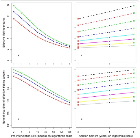
Figure 5Effective lifetime of a mass LLIN distribution, depending on pre-intervention EIR and attrition half-life. Entomological inoculation rate (EIR) is defined as infectious bites per adult per annum (ibpapa). Attrition half-life (years): red lines and crosses = 3, blue lines and crosses = 4, green lines and crosses = 5. Figures c & d EIR: dashed black lines = 2, dashed red lines = 4, dashed green lines = 8, dashed blue lines = 16, light blue lines = 32, magenta lines = 64, yellow lines = 128, grey lines = 256. Figures a & c) Effective lifetime on vertical axis, Figures b & d) Natural logarithm of effective lifetime on vertical axis.

Briëtet al.Malaria Journal2012,11:20 http://www.malariajournal.com/content/11/1/20

distribution will last. Following intervention, the impact on clinical malaria incidence reaches a maximum within a short period and is sustained for some time, after which the number of episodes rises steeply. Clearly, re-intervention (LLIN distributions or other) should take place before case incidence exceeds pre-intervention levels (due to the loss of acquired immunity). The‘ effec-tive lifetime’, defined as the period from intervention until the reduction in incidence falls to a set cut-off pro-portion of the maximum impact, can be used to decide when to re-intervene. Because of the sharp rise in inci-dence it matters little whether the cut-off is set at 40, 50 or 60% of the maximum, and there is little interaction between the cut-off value and the effect of the pre-inter-vention EIR, indicating that the sensitivity analysis would probably give similar results if a cut-off other than 50% had been used. Even though optimal criteria for determining when to re-intervene would include economic factors, the use of the‘effective lifetime’thus provides a reasonably robust alternative.

Pre-intervention EIR level

LLINs have approximatelya the same proportionate effect on vectorial capacity at different pre-intervention EIRs. However, the apparent rate at which malaria transmission resurges from a level lower than its steady state is strongly positively related to vectorial capacity. High resurgence rates appear to be associated with shal-lower minima in the annual number of episodes and in the annual number of (asymptomatic) infections, but this observation results mainly from temporal smoothing.

Depending on the pre-intervention EIR, three model variants showed very different effective lifetimes from the base modelR0000. These are modelsR0063,R0065, and R0068, in which the age-specific susceptibility is independent of exposure (contrasting with the sigmoidal relationships with exposure in the other variants), and that include extra-Poisson variation in the probability of being bitten. Model R0063assigns most of this to inter-host variation; model R0065is intermediate, and model R0068 assigns the variation predominantly to ‘within host variation’, assuming that some individuals are always more likely to get bitten than others [10]. An explanation for why these model variants have different results is outside the scope of this paper. The models R0063 and R0065, both with inter-host variation in exposure, showed a stronger relationship between effec-tive lifetime and pre-intervention EIR than did the base model. Heterogeneity in exposure to infectious bites between individuals is highly likely, as there are differ-ences in mosquito access to houses [16] (depending on house quality and geographical situation) and in indivi-dual attractiveness to mosquitoes [17,18]. The effect of

Figure 6 Effective lifetime of a mass LLIN distribution, depending on initial coverage and model variant. Initial coverage is the percentage of people that received access to an LLIN at the time of distribution. All parameters other than initial coverage are at central values. Model variants are coloured as indicated in Figure 4.

pre-intervention EIR is thus possibly even stronger than shown in the sensitivity analysis, based on averages of 14 model variants, 12 of which ignore inter-host varia-tion in exposure.

For the sake of simplicity, results in the sensitivity analysis were averaged over 14 model variants. This can be problematic if there is strong interaction between the effect and the model over the range studied, as was the case with the pre-intervention EIR. Sensitivity to cover-age, however, was similar for all model variants.

Although the 14 model variants reflect a plausible range of models, they are not necessarily evenly spread out over this range. In order to calculate a mean effect, models should ideally be weighted based on their overall fit, and on correlations between both structure and parameter values with other variants in the ensemble. Model variants with a poor fit, and/or similar to other variants included in the analysis, should receive a low weight. To perform such a weighting is a challenging task and there is a need for more methodological

Figure 8Ratio of annual episodes in a situation with LLIN sustained coverage without attrition or decay to a situation without LLINs, depending on pre-intervention EIR and coverage. Each green line represents the median number of episodes of 10 simulation runs (each with unique random seed) with LLINs distributed to the people (population size = 10,000) at the beginning of year 6, the number of episodes in each intervention simulation run divided by the number of episodes in a simulation run without LLINs (also with unique random seed). The red semi transparent polygons represent the range of the 10 runs. Per panel, there are 14 green lines (and 14 red polygons), each representing a malaria model variant. The first column of panels (a-c) shows results for 60% coverage and the second column (d-f) for 80% coverage. The panel rows show results for pre-intervention EIRs of 16 (a & d), 32 (b & e), and 256 (c & f) ibpapa. Blue lines represent the proportion of people using an LLIN, added to one. Horizontal lines: dashed, ratio = 1; dotted, ratio = 0.

Briëtet al.Malaria Journal2012,11:20 http://www.malariajournal.com/content/11/1/20

development in this area to address the problem appropriately.

In all the model variants, pre-intervention EIR was varied by scaling vector emergence rates. The pre-inter-vention EIR could possibly also be varied by changing other variables influencing vectorial capacity, such as intervention survival rate, and such a

pre-intervention EIR may have a somewhat different rela-tionship with the LLIN effective lifetime.

Vector emergence was modelled as a fixed repeating seasonal pattern, independent of the adult vector popu-lation size. If the models were to include feedback from the reduced vector population due to interventions, leading to fewer emerging mosquitoes, then longer

effective lifetimes would be expected, especially at loca-tions with lower emergence rates (where local extinction of vectors might occur). Therefore, these models give a conservative estimate of effective lifetime and its depen-dency on emergence rates.

LLIN decay

Effective lifetime is highly sensitive to the attrition rate. With a short attrition half-life, nets disappear before net decay can have much impact. Hole formation and insec-ticidal content decay are therefore of more importance with slower attrition rates. In turn, variability in hole rate and insecticide decay rate, hole size (rip factor) and the effects of decayed nets on mosquito biting and sur-vival, are only important when hole formation and insecticidal content decay are themselves important. Thus, the shorter the attrition half-life, the more impor-tant is its accuracy relative to that of the other net decay parameters.

Insecticide decay rate is conditional on slow attrition and one of the most important factors determining the effective lifetime of an LLIN distribution. Lifetime varies strongly between the lower half-life estimate (0.5 years, characteristic for first generation LLINs) and the central value (1.5 years, characteristic for second generation LLINs). Insecticide half-life is strongly product-depen-dent and the values for specific products are relatively well-defined, so, despite its importance, insecticide decay is not a major contributor to uncertainty in effec-tive lifetime, provided that mosquitoes remain sensieffec-tive

to the active compound. It remains to be studied how sensitive the effective lifetime of LLINs will be to this parameter in the presence of pyrethroid resistance [19].

Effective lifetime of an LLIN distribution was surpris-ingly insensitive to parameters specifying the hole for-mation process in the nets. It is possible that the guessed values for theholeScalingFactor, not based on any data, were unreasonable, and that the effect of LLINs on mosquitoes wanes much faster than presumed as the hole index increases. Even though insensitive to hole parameters, it would still be useful to have evi-dence-based estimates as, with the emergence and spread of pyrethroid resistance [20-22], tear resistance is expected to gain in relative importance.

Coverage

Coverage targets can be varied relatively easily in mass distribution campaigns, thus the effects of coverage were examined in more detail. But, effective lifetime was found to be insensitive to the initial coverage, expressed as the percentage of people that had access to an LLIN at the time of distribution. Since simulated people were not grouped into households, where they could share commonly owned nets, each covered person was simu-lated independently with a distinct net, used every night. This precluded explicit modelling of the distinction between household ownership of nets and personal net use, net transfer patterns within families, or local pro-tective effects shared between net users and non-users [23]. Thus the simulated coverage is equivalent to the percentage of people that used an LLIN. However, the insensitivity of effective lifetime to coverage implies that it would also be insensitive to measures of usage or familial correlations in ownership or usage.

The simulation experiment with sustained net cover-age sheds some light onto what might happen if mass LLIN distributions are repeated at regular intervals, or supplemented by LLIN distribution through continuous delivery channels, such as the Expanded Program on Immunization (EPI). Although the assumption of no net attrition or decay is unrealistic, this experiment allows to distinguish the effects of attrition and decay from the transient dynamics induced by reducing exposure.

In settings with a medium to high pre-intervention EIR, after initial reduction the episode incidence will increase over time even in the absence of decay in num-ber and state of LLINs, and reach a new equilibrium that is higher than its minimum. This is due to a reduc-tion in the equilibrium level of acquired immunity caused by the reduction in exposure. The rate of decline in prevented episodes with sustained coverage is rela-tively slower than with a mass distribution with a four-year attrition half-life and central values for decay of both net coverage and physical and chemical states of

Figure 10Equilibrium ratio of episodes with LLIN sustained coverage to episodes without intervention, depending on pre-intervention EIR and coverage. Coverage (%): light blue (40), magenta (50), red (60), blue (70), green (80). The dotted horizontal line indicates a ratio of 1.

Briëtet al.Malaria Journal2012,11:20 http://www.malariajournal.com/content/11/1/20

the nets. For instance, at pre-intervention EIR of 128 ibpapa, with 70% coverage, for sustained coverage and for a mass distribution, the effective lifetimes were 15.8 and 3.0 years, respectively. This suggests that a decline in natural immunity has little impact on the effective lifetime of a single mass LLIN distribution.

Over a long period, lower acquired immunity levels will reduce the number of clinical episodes prevented by LLINs and will be accompanied by a shift in the age dis-tribution of the clinical episodes. Some of the simulations suggest that prolonged low coverage levels in areas with a high pre-intervention EIR could lead to an increase in incidence that exceeds pre-intervention levels. However, many of the episodes in these simulations occur in older children or adults, and may well be milder than had they occurred at younger ages, resulting in overall lower case fatality. Nevertheless, these results suggest that a sus-tained high level of coverage of 80% could continue to suppress episodes at medium pre-intervention EIRs of 128 ibpapa and below, despite (complete) loss of acquired immunity. This supports high coverage targets for long-term sustained intervention planning. However, a sepa-rate simulation study involving multiple distribution mechanisms, such as antenatal care and EPI continuous distribution and repeated mass distributions, would be required before answering the question“what target cov-erage is most cost effective?”.

Conclusions

The strong dependency of the effective lifetime of an LLIN mass distribution on pre-intervention transmission indicates that the required distribution frequency may vary more with the local entomological situation than with LLIN quality or the characteristics of the distribu-tion system. This highlights the need for monitoring malaria before and during intervention programmes, par-ticularly since there are likely to be strong variations between years and over short distances. The majority of sub-Saharan Africa’s population probably falls into expo-sure categories where the effective lifetime is relatively long [24], but because exposure estimates are highly uncertain, it is necessary to consider subsequent control measures sooner than at the end of the expected effective lifetime based on an imprecise measure of transmission.

Endnotes

a

Only different death rates might influence LLIN owner-ship, and thus LLIN effect on the vectorial capacity.

Appendix

Experiment parameterisation of ITN effects in OpenMalaria and experiment parameter values

In this Appendix, for selected parameters (italicised) and parameter groups (italicised) important for this study,

detailed information is given on the choice of the para-meter values.

The discussion of the parameters and parameter groups is organised according to the hierarchical organi-sation of a scenario script. The experiment’s ‘central’ scenario specification in the machine readable language XML is given as Additional file 1, and also on the OpenMalaria site [15]. This XML scenario is richly annotated to explain what function the parameters have. Additional information on the function of the para-meters is documented in the wiki section of the project webpage [6]

demography

The ‘Ifakara’demography [25] was used. The population is stationary and approximately stable: individuals move up in age group with time, and because this structure is monotonically decreasing with age, surplus individuals are out-migrated (also abovemaximumAgeYrs).

popSize

A population size (popSize) of 10,000 was used. This is a balance between computational effort (which increases with larger population size) and the level of stochasticity (which decreases with larger population size). At a size of 10,000, the effect of rounding integers in the popula-tion demography (which is noticeable below a size of 5,000) is minimal.

monitoring

For this study, the following output variables are rele-vant:nets owned: the total number of nets (irrespective of physical and chemical state) present in the popula-tion; nUncomp: the number of uncomplicated malaria episodes; nSevere: the number of complicated, severe malaria episodes; nNewInfections: the number of new infections.

interventions > ITN > usage value

Usage represents the proportion of time during the night that a net is used by a simulated individual. It is not the proportion of people that use a net conditional on ownership. Because, in the current model, mosquito species bite homogenously throughout the night, the usage value can also be interpreted as the probability that host searching occurs during the time that people who own a net are using the net. In literature, this is called the ‘πi value’ [26]. Govella and colleagues [27]

define it as “the proportion of normal exposure of unprotected humans lacking nets that occurs at times and places when net users would be protected by sleep-ing under them”. The current model version (schema 29) allows only oneusage value to be set, thus it is not possible to vary theπivalue for different species within

the same scenario through theusage value, nor can the usage valuebe varied over net users.

probability to search in places during times when people are protected by a net (if they own one). This, as opposed to situations where the mosquito population might be, to a degree, divided into sub-populations which either always or never search only during times and in places when people are protected by a net. Such separate behaviour could be caused by genetics, and by learning; repeating the behaviour of whatever happened in the first feeding cycle.

Comparisons of indoorversusoutdoor human landing catches throughout the night, combined with studies of human behaviour and the source of blood meals, give insights into the proportion of host searching mosqui-toes that would encounter an ITN protected host (given ownership). However, the degree to which sub-popula-tions exist that display different behaviours is unknown.

This parameter was varied for the sensitivity analysis. A usage valueof 0.75 was used as the central value, assum-ing high endophagy (the propensity to bite indoors) and biting peaks after average bed-time of the population. The extreme low parameter value was taken as 0.5 and the extreme high value was taken as 1.0. These values are based on theπivalues reported by Govella and colleagues

[27] and Russell and colleagues [28]. interventions > ITN > holeRate mean

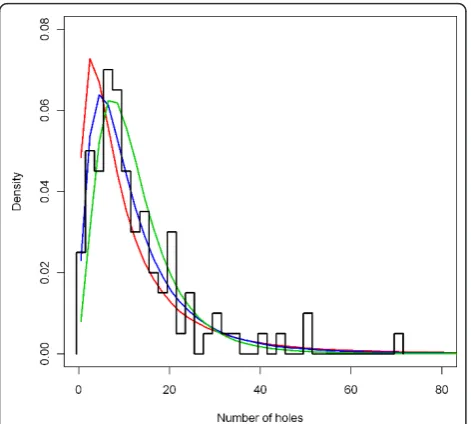
The level of the annual hole formation rate of nets, the holeRate mean, was set at 1.8 holes per net per year. This value was based on re-analysis of the data on dis-tribution of the total number of holes in Olyset nets after seven years of use [29], provided by Christian Len-geler. An outline normalised histogram of this distribu-tion is shown in Figure 11. This parameter was varied for the sensitivity analysis. The extreme low parameter value was taken as 0.9 (half of the central value) and the extreme high value was taken as 3.6 (double of the cen-tral value). The effects of these parameters are also shown in Figure 11.

interventions > ITN > holeRate sigma

The value of the hole formation rate is varied among nets by multiplying with a distribution factor which is log nor-mally distributed with mean one and the standard devia-tion of the log transformed variable sigma). The distribution factor is generated by taking one sample per net from a Gaussian distribution with mean zero and standard deviation one. For each parameter (holeRate, ripRate,insecticideDecayrate), the same sample is multi-plied by the respectivesigmaand a constant (mu) added such that, once exponentiated, the mean of the variable over nets is one. ForinsecticideDecayrate, this constant can be chosen freely. The transformed sample is then exponentiated to obtain the respective distribution factor. This procedure implies that the distribution ofholeRate, ripRateand insecticide decay rate are supposed to be covariant: nets that are heavily used decay fast both

chemically and physically, whereas nets that are gently used decay slowly both chemically and physically. There is some evidence that these are indeed associated [30].

The central level of the sigmaparameter of the distri-bution factor for hole formation rates was set to 0.8. This value was also based on re-analysis of the raw data on distribution of the total number of holes in Olyset nets after seven years of use [29], provided by Christian Lengeler. The holeRate sigmaparameter was varied for the sensitivity analysis (Figure 12). The extreme low parameter value was taken as 0.60 and the extreme high value was taken as 1.00.

interventions > ITN > ripRate mean

The ripRate meanvalue was set equal to the value of theholeRate mean. (The ripping process was assumed to be similar to the hole formation process). This para-meter was thus varied for the sensitivity analysis, but not independently.

interventions > ITN > ripRate sigma

Theriprate sigmavalue was set equal to the value of the holeRate sigma. (The ripping process was assumed to be similar to the hole formation process). This parameter was thus varied for the sensitivity analysis, but not independently.

interventions > ITN > ripFactor value

TheripFactor valueexpresses how important rips are in increasing the (proportionate) hole index. A net’s hole

Figure 11Distribution of the number of holes after seven years, depending onholeRate mean. The black line represents a normalised outline histogram showing the density function of the number of holes as counted by Tami and colleagues [29] in 100 nets. The coloured lines represent the normalised histogram mid-points of the number of holes in simulated nets depending on the

holeRate mean, which is varied over 0.9 (green), 1.8 (blue) and 3.8

(red), with a constantholeRate sigma(see below) of 0.80. Briëtet al.Malaria Journal2012,11:20

http://www.malariajournal.com/content/11/1/20

index is the hole count plus the ripFactor value multi-plied with the cumulative number of rips. With the cen-tral values for holeRate mean, ripRate mean, holeRate sigma and ripRate sigma, a ripFactor value of 0.30 allowed to approximate the upward curve in the mean hole index shown by Kilian and colleagues [31] (See Fig-ure 13). Based on this, the central level of theripFactor value was set to 0.30. Extreme low and extreme high values were chosen of 0.15 and 0.60, respectively. interventions > ITN > initialInsecticide mu

The mean insecticide content of new nets ( initialInsecti-cide mu) is set to 68.4 corresponding to the declared deltamethrin content of 68.4 mg.m-2 for long-lasting (incorporated into filaments) insecticidal nets according to WHO interim specification 333/LN/3 [32].

interventions > ITN > initialInsecticide sigma

The insecticide concentration of new nets is Gaussian distributed. The standard deviation (sigma) was set to 14, based on the interquartile range observed by Kilian and colleagues [31], for Permanet 2nd generation. interventions > ITN > insecticideDecay L and function The insecticideDecay functionchosen was“exponential”,

φt=exp

−tln(2)

L

with t the proportion of the

initial insecticide concentration remaining at time t(in years). The insecticideDecay Lparameter then directly translates into the insecticide half-life in years. However,

if the decay ratel= ln(2)/Lis heterogeneous, the mean half-life is longer (Figure 14). The insecticideDecay L parameter was varied for the sensitivity analysis. The central level of theinsecticideDecay L for the decay rate of the insecticide in the nets was taken as 1.5, which, if combined with a central distribution factor insecticide-Decay sigmaof 0.8, yields a mean half-life of about two years. This roughly corresponds to the decay of second generation LLINs [30,31], The extreme low parameter value was taken as 0.5, roughly corresponding to first generation LLINs. The extreme high value was taken as 2.5.

interventions > ITN > insecticideDecay sigma (and mu) The parametersinsecticideDecay mu and insecticideDe-cay sigmaare for the distribution factor (same samples as for theholeRatedistribution factor). Figure 15 shows how the variation in the insecticide increases over time due to the heterogeneity in the insecticide decay rate l. Such behaviour is also apparent from data presented by Killian and colleagues [31]. TheinsecticideDecay sigma was varied for the sensitivity analysis. The central level ofinsecticideDecay sigma was chosen at 0.8 and insecti-cideDecay muwas chosen such that the mean was equal to one (insecticideDecay mu = -0.32 for the central value). The extreme low parameter value was taken as 0.60 and the extreme high value was taken as 1.00. Fig-ure 16 shows the distribution of the percentage insecti-cide remaining at 38 months. Figure 16a looks similar to Figure 6 presented by Smith and colleagues [33] for first generation LLINs. Figure 17 shows the density of

Figure 12Distribution of the number of holes after seven years, depending onholeRate sigma. The black line represents a normalised outline histogram showing the density function of the number of holes as counted by Tami and colleagues [29] in 100 nets. The coloured lines represent the normalised histogram mid-points of the number of holes in simulated nets depending on the

holeRate sigma, which is varied over 0.6 (green), 0.8 (blue) and 1.0

(red), with a constantholeRate mean(see above) of 1.8.

Figure 13 Mean hole index over time as a function of the

ripFactor value. Coloured lines plotted on the right hand vertical axis represent the mean hole index depending on theripFactor

value, which was varied over 0.6 (green), 0.3 (blue) and 0.15 (red),

insecticide concentration in nets over time, with all parameters at central values.

interventions > ITN > attritionOfNets L and function and k The attrition function used is “smooth-compact”,

ψt=exp

k− k

1−tL2

with t the proportion of

the initial net coverage remaining at timet(in years). A kvalue of 18 was used. The smooth-compact function with this kvalue was applied by Nakul Chitnis to data on net ownership provided by Albert Kilian (Chitnis and Kilian, personal communications). TheLparameter was varied for the sensitivity analysis and chosen such that 50% of nets initially distributed had disappeared after 3 (low extreme), 4 (central level) or 5 (high extreme) years. This was at L values of 15.579, 20.773 and 25.966, respectively. It should be noted that from the simulated population, which is kept at a stationary size, people are out-migrated (with their nets) due to population growth. Therefore, the attrition rate of nets per person in the simulated population is slightly higher than the attrition of nets (Figure 18); if the half-life of the attrition of nets would be infinity, with a population growth of 3.47%, the half-life of nets per person in the simulated popula-tion would be about 20 years. Populapopula-tion growth may thus explain part of the observed difference in attrition rates between prospective studies (cohort based) and population wide surveys.

interventions > ITN > anophelesParams

For this experiment, effects of ITNs on anopheline mosquitoes were assumed to be equal for all vector species. The mosquito gonotrophic cycle as modelled in the OpenMalaria vector component [8,9] is illu-strated in Figure 19. Female mosquitoes enter the hun-gry state either after emergence or after successfully ovipositing. Then they start host tracking, where they either do not encounter a host (and will continue host

Figure 14Mean percentage insecticide remaining over time as a function ofinsecticideDecay L. The coloured lines represent the insecticide remaining over time, as a percentage of the initial concentration, depending on theinsecticideDecay L, which is varied over 0.5 (red), 1.5 (blue) and 2.5 (green), with ainsecticideDecay

sigmaat the central value of 0.8 (solid lines), or at 0 (dotted lines).

Figure 15Percentage insecticide remaining over time with all parameters at central values. The grey polygon represents the interquartile range, the solid blue line represents the median and the dashed blue line represents the mean.

Briëtet al.Malaria Journal2012,11:20 http://www.malariajournal.com/content/11/1/20

tracking the next night) with probability PA, die in the process with probability PA μ, or encounter a host of typei (PAi).

After encountering a host of type i, they determine whether to attack or not (in which case they continue host tracking). These terms are not separately modelled, and included inPAiandPA, respectively. In this model,

once a mosquito is determined to attack, it will either successfully feed, or die in the process. Unfed alive (UA) mosquitoes found in experimental huts are thus regarded as those that encountered a host and entered the hut but decided not to attack. This is a simplifica-tion of reality, where a mosquito may survive after unsuccessfully trying an attack. Deterrency acts on the determining phase. Deterrency is defined as one minus the relative number of affected mosquitoes (RA1 vs 2) of

a host of type 1, as compared to another host of type 2. The number of affected mosquitoes is calculated as the sum of fed alive (FA), fed dead (FD) and unfed dead (UD) mosquitoes. A host type that is protected by an ITN will likely have a ratio below one, relative to a simi-lar host type without ITN protection.

A mosquito determined to attack host i will either succeed in inserting its proboscis with probability PBi,

or die during the process without inserting its proboscis, with probability PBμi. For transmission from mosquito

to human, it is important that the proboscis is inserted, and not if blood feeding was successful. However, in OpenMalaria, for simplicity, only blood-fed mosquitoes are assumed to have potentially inoculated hosts with sporozoites. ITNs will have an effect on the pre-prandial killing probability PBμi, which can be approximated by

the proportion of UD mosquitoes out of the total of determined (unfed dead, and fed dead or alive) mosquitoes.

After proboscis insertion, feeding takes place and the mosquito tries to escape from the host’s vicinity, which is successful with probability PCi, or unsuccessful and

the mosquito dies in the process. ITNs will have an effect on the probability of successfully escaping the host after a blood meal, called the post-prandial killing effect. This can be approximated by the proportion of FD mosquitoes out of the total of fed (dead or alive) mosquitoes.

Having escaped the host’s vicinity, the mosquito will search for an appropriate resting spot. An ITN might interfere with this (through an excito-repellent effect), but this was not modelled specifically.

After a mosquito finds a resting spot it rests, and sur-vives with probability PDi. Whereas indoor residual Figure 16Distribution of the percentage insecticide remaining

of the initial concentration, after 38 months, depending on

insecticideDecay LandinsecticideDecay sigma. The coloured lines represent the normalised outline histogram of insecticide remaining as a percentage of the initial concentration in simulated nets depending on theinsecticideDecay sigma, which is varied over 1.0 (green), 0.8 (blue) and 0.6 (red), and oninsecticideDecay L, which is varied over 0.5 (a), 1.5 (b) and 2.5 (c).

Figure 17Density of insecticide concentration over time, with all parameters at central values. Three dimensional plot with the proportional distribution (density) of nets over categories of insecticide concentration in 10 mg.m-2_{intervals, with lines at}

category mid-points. At time zero, the insecticide concentration is Gaussian distributed over the nets with mean 68.4 and standard deviation 14, but as the insecticide decays over time, the distribution is no longer Gaussian due to heterogeneity in the

insecticideDecayrate. After 20 years, 77% of the nets has a

spraying acts during this phase, ITNs were assumed to have no influence here. Experimental hut study proce-dures will typically collect mosquitoes in the morning (before the resting is complete), and observe alive mos-quitoes for an extended period to account for deaths during the resting phase. This is because contact with insecticide picked up during earlier phases may have a delayed effect on mortality.

Rested mosquitoes will search for an oviposition site, ovi-posit and start another gonotrophic cycle by host tracking.

ITNs give both personal protection by reducing the number of (infectious) bites, and reduce transmission by reducing the mosquito survival per gonotrophic cycle through increased mortality during attack and escape phases, and more time spent host tracking (with asso-ciated mortality) due to deterrency.

In the ITN model, new ITNs can decay both physi-cally (formation of holes) and chemiphysi-cally (loss of sur-face-active ingredient). Published experimental hut studies testing ITNs have typically several (non stan-dard) trial arms, sometimes including no-net control host types (NN), intact untreated net host types (IU), intact insecticide treated net host types (IT), deliberately holed insecticide treated net host types (HT), and holed untreated net host types (HU). These trial arms (Table 1) are of interest as they allow estimating parameter

values for the effects of ITNs depending on their (extreme) physical and chemical states. Four references [11-14] were selected, containing six hut experiments with a no-net control and two or more of the other trial arms of interest, and for which the relative proportions of mosquitoes in the UA, UD, FA and FD categories could be retrieved, either from data tables or figures. Note that different authors use different hole numbers and sizes,e.g.: 8 holes of 10 × 20 cm [12]; 6 holes of 10 × 5 cm [11]; 6 holes of 10 × 10 cm [14].

interventions > ITN > anophelesParams > deterrency The relative number of affected mosquitoes in trial arms with a mosquito net as compared to no net, from sources in literature, are displayed in Table 2.

Gokool and colleagues [14] and Curtis and colleagues [11] (in their second experiment) found more fed and/or deadAnopheles gambiaes.l. in huts with untreated, holed mosquito nets than without nets. Clearly this is an artefact caused by imperfect hut traps, with more mosquitoes escaping from huts without nets, than from huts with nets, where mosquitoes got trapped under the net. It is extre-mely unlikely that a holed untreated net makes a person more attractive to mosquitoes than when without a net.

The geometric mean data suggest that 0.5 might be a reasonable central value for the RA of IU and IT host typesversus NN, and 0.67 a good central value for an HT host type. As explained above, if the HU host type is considered not to increase the number of affected mosquitoes, a central value of 1 seems reasonable. These values were used to compute the‘medium’ deter-rencyparameter group setting values.

The highest RA values were 0.78, 0.79 and 0.77 for IU, HT, and IT host types, respectively. These values were used to compute the ‘low’deterrency parameter group setting values.

The lowest RA values were 0.41, 0.55 and 0.35 for IU, HT, and IT host types, respectively. These values were used to compute the ‘high’deterrencyparameter group setting values.

If linear relationships are assumed between the loga-rithm of the RA and the active insecticide concentration (p) and hole index (h), where pis scaled from zero (no insecticide) to one (maximum active surface concentra-tion for a new ITN) and h(which could be expressed as the number of holes, a composite hole index based on number and size of holes, or holed surface in cm2or as a percentage) is scaled from zero (intact) to one (badly torn net), these could be written as follows:

RAivs NN= exp ⎛ ⎜ ⎝

log(holeFactor) (1−h)+ log(insecticideFactor)p+ log(interactionFactor) (1−h)p

⎞ ⎟

⎠, where:holeFactor= RAIU vs NN,

insecticideFactor= RAHT vs NN, andinteractionFactor= RAIT vs NN

RAIU vs NN×RAHT vs NN

.

Figure 18 Percentage of LLINs remaining over time. The coloured lines represent the LLINs remaining over time after a mass distribution, as a percentage of the initial number, depending on

theattritionOfNets L, which is varied over 15.579, 20.773 and 25.966,

with half-lives of 3 (red), 4 (blue) and 5 (green) years, respectively. Solid lines are for the percentage of nets with as denominator the number of people remaining in the population cohort that initially received LLINs. Dashed lines are for the percentage of nets with as denominator the total (growing) population, presuming an initial coverage of 100%.

Briëtet al.Malaria Journal2012,11:20 http://www.malariajournal.com/content/11/1/20

However, it was assumed that the relationships between the log of the RA and insecticide and holes are not linear, but increases asymptotically as the number of holes increase, and the insecticide concen-tration decreases. Thus the following relationship was used:

RAivs NN= exp

⎛ ⎜ ⎝

log(holeFactor)exp−h×holeScalingFactor+

log(insecticideFactor)1−exp−p×insecticideScalingFactor+

log(interactionFactor)exp−h×holeScalingFactor 1−exp−p×insecticideScalingFactor

⎞ ⎟ ⎠

,whereholeScalingFactor andinsecticideScalingFactor are scaling factors for the number of holes, and the insecticide concentration, respectively. The

holeScalingFactor andinsecticideScalingFactordescribe how fast the effect of the hole index, and insecticide concentration, respectively, plateaus. For the ‘medium’ deterrencylevel this is:

RAivs NN= exp

⎛ ⎜ ⎝

log(0.5)exp−h×holeScalingFactor+ log(0.67)1−exp−p×insecticideScalingFactor+ log 0.5

0.5×0.67

exp−h×holeScalingFactor 1−exp−p×insecticideScalingFactor

⎞ ⎟ ⎠

This relationship is illustrated in Figure 20.

Figure 21 illustrates the ITN effects ondeterrencyfor all three modelled levels (low, medium, and high).

Although theholeScalingFactorand the insecticideSca-lingFactor can be specified for each ITN effect (

deter-rency, preprandialKillingEffect and

postprandialKillingEffect) separately and for each mos-quito (sub) population or species separately, the same holeScalingFactorandinsecticideScalingFactor were used for ITN effects and species in these simulations.

There is little information available in literature to inform the choice for a reasonable value for the holeSca-lingFactor and the insecticideScalingFactor. For the insecticideScalingFactor, the dose-response curve of insecticide on killing in WHO cone tests [31,34] was used. Figure 22 shows such a relationship for deltame-thrin (adapted from [34], Figure 4A, page 40), with the deltamethrin concentration expressed in mg.m-2 (by

multiplying the g.kg-1scale with 85/2.8). Based on the shape of the relationship between the proportion of dead mosquitoes after contact with insecticide in the WHO cone tests, depending on deltamethrin concentra-tion, the value of 0.1 was chosen as the central value, 0.2 was chosen as the high extreme value, and 0.05 was chosen as the low extreme value. This is largely in agreement with experimental hut data presented by Lindsay and colleagues [35] for killing and deterrency. However, the solvent proved to be highly deterrent in that study, making it difficult to use the results to pre-dict the deterrency of aged netsversusnew nets.

For holes, very little information was available. Carne-vale and colleagues [36] published data over a range of physical damage to nets (0.5, 1 and 2% of the net sur-face) and number of bites, but the relationships varied over the experiments. For this work, the same range of values for theholeScalingFactoras used for the insectici-deScalingFactorwas chosen: 0.05, 0.1 and 0.2.

Figure 23 illustrates the ITN deterrent effects for the mediumdeterrency level, with the three modeled para-meter values for theholeScalingFactorand the insectici-deScalingFactorvaried simultaneously.

interventions > ITN > anophelesParams > preprandialKillingEffect

The pre-prandial killing in trial arms from sources in lit-erature are displayed in Table 3.

Table 1 Host types used

Abbreviation Host type

NN Person without a net

IT Person with an intact treated net

IU Person with an intact untreated net

HT Person with a holed treated net

HU Person with a holed untreated net

HsatT Person with a treated net, holed to saturation

HsatU Person with an untreated net, holed to saturation

θT Person with a treated net, with undefined hole index

θU Person with an untreated net, with undefined hole index

Table 2 Relative number of affected mosquitoes by host type

Reference NN IT IU HT HU Holes

[11] EXP 1 1 0.446 0.779

[11] EXP 2 1 0.682 1.258 6 h, 10 × 5 cm

[11] EXP 3 1 0.549 6 h, 10 × 5 cm

[12] 1 0.552 0.465 0.682 1.025 8 h, 10 × 20 cm

[14] 1 0.769 0.790 1.325 6 h, 10 × 10 cm

[23] 1 0.345 0.410

geometric mean 1 0.506 0.530 0.670 1.195

Relative number of affected mosquitoes by host type compared to no net.h

= holes;EXP= experiment; other abbreviations as in Table 1.

Figure 20Modelled relationship between relative number of affected mosquitoes and insecticide concentration and hole index for the‘medium’deterrencylevel. In this figure, insecticide concentration is varied between 0 and 100 mg.m-2, and the hole index is varied between 0 and 50. The scaling factor for holes and insecticide (holeScalingFactorandinsecticideScalingFactor, respectively), are both set to 0.10.

Briëtet al.Malaria Journal2012,11:20 http://www.malariajournal.com/content/11/1/20

In order to calculate a standardised effect, corrected for different mortality in the NN host type arm, prob-ably due to varying environmental and experimental conditions, the following process was adopted:

All proportions were logit transformed and the aver-age value for NN host types was calculated. For each experiment, the difference between the logit NN value and the average logit NN value was subtracted from the logit value of all other treatments. Then, the average for each treatment over all experiments was taken and back transformed into a proportion (Table 4).

The mean proportion killed for NN host types was lowest (0.09), and the mean proportion for HU host types was somewhat higher (0.23). IU host types had a much larger proportion killed (0.66), followed by HT host types (0.73) and IT host types (0.84).

The fact that the average proportion killed for HU host types (0.23) was higher than that of NN host types (0.09) indicates that holed untreated nets do have a small effect on pre-prandial killing, despite the (severe) damage done to the nets. If the nets were damaged even more, the effect would presumably be smaller and even-tually, at a saturation point, such a net (host type HsatU), would no longer impede flight of mosquitoes and the pre-prandial mortality would be the same as for NN. It is of interest to estimate the effect of the

Figure 21Modelled relationship between relative number of affected mosquitoes and insecticide concentration and hole index, depending ondeterrencylevel. In this figure, insecticide concentration is varied between 0 and 100 mg.m-2_{, and the hole}

index is varied between 0 and 50. The scaling factor for holes and insecticide (holeScalingFactorandinsecticideScalingFactor,

respectively), are both set to 0.10. Top layer: lowdeterrency; middle layer: medium leveldeterrency, bottom layer: highdeterrency.

Figure 22Relationship ofAnophelesmortality in WHO cone tests with deltamethrin concentration, and modelled

relationship. Black circles represent observations adapted from Figure 4A, page 40, in the report of the twelfth WHOPES working group meeting [34]. The coloured lines represent modelled relationship mortality = 1 - exp(-p×insecticideScalingFactor) withp

the insecticide concentration and with values for

insecticideScalingFactorof 0.05 (red), 0.1 (blue) and 0.2 (green).

Figure 23Modelled relationship between relative number of affected mosquitoes and insecticide concentration and hole index for the‘medium’deterrencylevel, depending on

insecticide at this saturation point, thus for treated nets holed to saturation (HsatT). Presumably, the effect of an HsatT net would be similar to sleeping next to, not under an HT net. If the effect decays with the same shape function (linear or exponential) for both untreated nets and treated nets, this can be calculated.

Let hdenote the hole index in a net in arbitrary units. The host typei can be described by the following letter combinations: NN, HU, IU, IT, HT, HsatT, HsatU, θT or θU (Table 1), depending on the net type the host uses. The letterθindicates here an undefined hole state. For example, if a linear decay in effect is presumed, if

hHsatU= 1 andhIU= 0, then PBμθU=PBμIU- (PBμIU

- PB μNN)hθU = 0.66 - (0.66 - 0.09)hθU. Thus, if PB

μHsatU = 0.23, then hHU= −(

0.23−0.66)

0.66−0.09 = 0.7544.

Then, if hHsaT = 1, hIT = 0, andhHT = hHU = 0.7544,

PBμHsatU=PBμIT−

PBμIT−PBμHT

0.7544 = 0.694. Thus the

values are 0.66, 0.69, 0.84, and 0.09 for IU, HsatT, IT, and HsatU host types, respectively. These values were used to compute the ‘medium’pre-prandial killing para-meter group values.

Similarly, the highest values are 0.83, 0.89, 0.93, and 0.09 for IU, HsatT, IT, and HsatU host types, respec-tively. These values were used to compute the ‘high’ pre-prandial killing parameter group values.

The lowest values are 0.44, 0.46, 0.72, and 0.09 for IU, HsatT, IT, and HsatU host types, respectively. These values were used to compute the‘low’pre-prandial kill-ing parameter group values.

WithPBμithe probability of dying before feeding as a

result of being committed to biting a host of typei, and pthe active insecticide concentration, with p= 1 the maximum active surface concentration for a new ITN, and p= 0 for an untreated net, if linear relationships between PB μi and pand hare assumed, these can be

written as follows:

PBμi=baseFactor+holeFactor(1−h)+insecticideFactor×p+interactionFactor(1−h)p,

wherebaseFactor=PBμHsatU;holeFactor=PBμIU−PBμHsatU, insecticideFactor=PBμHsatT−PBμHsatU,

interactionFactor=PBμIT−PBμIU−PBμHsatT−PBμHsatU.

For the medium preprandialKillingEffectlevel, this is thus: PBμi= 0.09 + 0.57(1−h)+ 0.60p−0.42(1−h)p. Note that for NN, PBμNN = 0.09, and that the

pre-prandial killing due to a net is the difference between PB μ1 (where the subscript 1 indicates a host type with

a net) andPBμNN.

Similar to the RA, it was assumed that the relation-ships between the preprandialKillingEffectand insecti-cide and holes are not linear, but decrease asymptotically as the number of holes increase, and increase asymptotically as the insecticide concentration increases. Thus, for the preprandialKillingEffect, the fol-lowing relationship was used:

PBμi=

baseFactor+holeFactor×exp−h×holeScalingFactor+ insecticideFactor1−exp−p×insecticideScalingFactor+

interactionFactor×exp−h×holeScalingFactor 1−exp−p×insecticideScalingFactor

For the mediumpreprandialKillingEffectlevel this is:

PBμi=

0.09 + 0.57×exp−h×holeScalingFactor+ 0.601−exp−p×insecticideScalingFactor−

0.42×exp−h×holeScalingFactor 1−exp−p×insecticideScalingFactor

This is illustrated in Figure 24.

Figure 25 illustrates the ITN effects on pre-prandial killing for all three modelled levels (low, medium, and high).

Figure 26 illustrates the ITN effects on pre-prandial killing for the medium level, with the three modelled parameter values for theholeScalingFactorand the insec-ticideScalingFactor, here both varied simultaneously. interventions > ITN > anophelesParams >

postprandialKillingEffect

The post-prandial killing in trial arms from sources in literature are displayed in Table 5, and the standardised values (see pre-prandial killing) are displayed in Table 6.

Table 3 Pre-prandial killing

Reference NN IT IU HT HU Holes

[11] EXP 1 0.170 0.89 0.79

[11] EXP 2 0.042 0.79 0.145 6 h, 10 × 5 cm

[11] EXP 3 0.156 0.65 6 h, 10 × 5 cm

[12] 0.033 0.62 0.63 0.49 0.120 8 h, 10 × 20 cm

[14] 0.100 0.94 0.71 0.150 6 h, 10 × 10 cm

[23] 0.140 0.81 0.56

Proportion of unfed dead mosquitoes out of the total of unfed dead, fed

dead and fed alive mosquitoes (pre-prandial killing).h= holes;EXP=

experiment; other abbreviations as in Table 1.

Table 4 Standardised pre-prandial killing

Reference NN IT IU HT HU Holes

[11] EXP 1 0.09 0.80 0.65

[11] EXP 2 0.09 0.90 0.28 6 h, 10 × 5

cm

[11] EXP 3 0.09 0.50 6 h, 10 × 5

cm

[12] 0.09 0.83 0.83 0.74 0.29 8 h, 10 × 20

cm

[14] 0.09 0.93 0.69 0.14 6 h, 10 × 10

cm

[23] 0.09 0.72 0.44

“back transformed mean of logits”

0.09 0.84 0.66 0.73 0.23

Standardised proportion of unfed dead mosquitoes out of the total of unfed

dead, fed dead and fed alive mosquitoes (pre-prandial killing).h= holes;EXP

= experiment; other abbreviations as in Table 1. Briëtet al.Malaria Journal2012,11:20 http://www.malariajournal.com/content/11/1/20