functional theory: Consequences of the approximations
.
White Rose Research Online URL for this paper:
http://eprints.whiterose.ac.uk/149472/
Version: Accepted Version
Article:
Archer, AJ, Ratliff, DJ, Rucklidge, AM orcid.org/0000-0003-2985-0976 et al. (1 more
author) (2019) Deriving phase field crystal theory from dynamical density functional theory:
Consequences of the approximations. Physical Review E - Statistical, Nonlinear, and Soft
Matter Physics, 100 (2). 022140. ISSN 1539-3755
https://doi.org/10.1103/PhysRevE.100.022140
©2019 American Physical Society . This is an author produced version of a paper
published in Physical Review E - Statistical, Nonlinear, and Soft Matter Physics. Uploaded
in accordance with the publisher's self-archiving policy.
[email protected] https://eprints.whiterose.ac.uk/
Reuse
Items deposited in White Rose Research Online are protected by copyright, with all rights reserved unless indicated otherwise. They may be downloaded and/or printed for private study, or other acts as permitted by national copyright laws. The publisher or other rights holders may allow further reproduction and re-use of the full text version. This is indicated by the licence information on the White Rose Research Online record for the item.
Takedown
If you consider content in White Rose Research Online to be in breach of UK law, please notify us by
consequences of the approximations
Andrew J. Archer,1,∗ Daniel J. Ratliff,1,† Alastair M. Rucklidge,2,‡ and Priya Subramanian2,§ 1
Department of Mathematical Sciences, Loughborough University, Loughborough LE11 3TU, U.K.
2
School of Mathematics, University of Leeds, Leeds LS2 9JT, U.K.
Phase field crystal (PFC) theory is extensively used for modelling the phase behaviour, structure, thermodynamics and other related properties of solids. PFC theory can be derived from dynamical density functional theory (DDFT) via a sequence of approximations. Here, we carefully identify all of these approximations and explain the consequences of each. One approximation that is made in standard derivations is to neglect a term of form∇ ·[n∇Ln], wheren is the scaled density profile andLis a linear operator. We show that this term makes a significant contribution to the stability of the crystal, and that dropping this term from the theory forces another approximation, that of replacing the logarithmic term from the ideal gas contribution to the free energy with its truncated Taylor expansion, to yield a polynomial inn. However, the consequences of doing this are: (i) the presence of an additional spinodal in the phase diagram, so the liquid is predicted first to freeze and then to melt again as the density is increased; and (ii) other periodic structures, such as stripes, are erroneously predicted to be thermodynamic equilibrium structures. In general,Lconsists of a non-local convolution involving the pair direct correlation function. A second approximation sometimes made in deriving PFC theory is to replace Lby a gradient expansion involving derivatives. We show that this leads to the possibility of the density going to zero, with its logarithm going to−∞ whilst being balanced by the fourth derivative of the density going to +∞. This subtle singularity leads to solutions failing to exist above a certain value of the average density. We illustrate all of these conclusions with results for a particularly simple model two-dimensional fluid, the generalised exponential model of index 4 (GEM-4), chosen because a DDFT is known to be accurate for this model. The consequences of the subsequent PFC approximations can then be examined. These include the phase diagram being both qualitatively incorrect, in that it has a stripe phase, and quantitatively incorrect (by orders of magnitude) regarding the properties of the crystal phase. Thus, although PFC models are very successful as phenomenological models of crystallisation, we find it impossible to derive the PFC as a theory for the (scaled) density distribution when starting from an accurate DDFT, without introducing spurious artefacts. However, we find that making a simple one-mode approximation for thelogarithm of the density distribution logρ(x) (rather than forρ(x)), is surprisingly accurate. This approach gives a tantalising hint that accurate PFC-type theories may instead be derived as theories for the field logρ(x), rather than for the density profile itself.
I. INTRODUCTION
The phase field crystal (PFC) theory for matter is widely used and has been successfully applied to de-scribe a broad range of phenomena, including, for exam-ple, grain boundary dynamics [1, 2], crystal nucleation [3, 4], crystal growth [5], glass formation [6], crack prop-agation [2] and many other properties of condensed mat-ter. For more background and examples of situations to which the PFC theory has been applied, see the excel-lent review [7]. The PFC theory was originally proposed, in the spirit of ‘regular’ phase field theory (PFT), as a diffuse-interface theory for the time evolution of an order parameter field [1]. The equations of PFT are obtained via symmetry, thermodynamic and other arguments and the result is a theory that is widely used in materials
∗Electronic address: [email protected] †Electronic address: [email protected] ‡Electronic address: [email protected] §Electronic address: [email protected]
science and other disciplines to model the structure of materials. For more background on PFT see for example Ref. [8] and references therein.
The central and original idea in extending PFT to ar-rive at PFC theory is to incorporate aspects of the micro-scopic structure of the material into the model [1]. The result is a theory that operates on atomic length scales and diffusive time scales [7]. By this we mean that PFC theory is a theory for a field that exhibits numerous max-ima, each of which is identified as the average location of the atoms (or more generally ‘particles’) in the sys-tem. This idea is powerful because, by building into the theory more information about the underlying material structure, it enables the inclusion of much more of the physics coming from particle correlations to be incorpo-rated. Over the years several variants of PFC theory have been developed that are able to describe a range different crystalline (and even quasicrystalline) structures [9–16].
dimen-sionless order parametern:
Fα[n] =
Z 1
2n (k 2
s+∇2)2−r
n+1 4n
4dx, (1)
wheren(x, t) is a field that depends on position in space x and on time t, and ks is an inverse length scale that
determines the lattice spacing of the crystal. The param-eter r defines how near the system is to freezing. The time evolution of the conserved field n is given by the dynamics
∂n ∂t =∇
2
δFα
δn
=−∇2 rn−(ks2+∇2)2n−n3
,
(2) where δFα
δn is the functional derivative ofFαwith respect
ton(x).
Given the ingredients in the model, it is therefore no surprise that PFC theory is closely related to the Swift– Hohenberg equation [17]:
∂n ∂t =−
δFα
δn =rn−(k 2
s+∇2)2n−n3, (3)
which is one of the archetypal equations in pattern for-mation theory. As one can see above, both the Swift– Hohenberg equation and PFC theory can be expressed as a different type of dynamics based on the same free energy functional [7]. The Swift–Hohenberg equation (3) is based on an underlying dynamics that seeks to min-imise the free energy over time, whilst the PFC dynam-ics (2), which also decreases the free energy over time, in addition enforces a conservation of the average value of the order parameter in the system. Thus, the PFC equation (2) is sometimes referred to as the conserved Swift–Hohenberg equation [7, 18–21].
In the years after PFC theory was originally proposed it was realised that it could be derived from classical dynamical density functional theory (DDFT) [5, 7, 22– 24], via a sequence of several different approximations. Below, we say much more on what these approxima-tions are. DDFT is a theory for the time evolution of the ensemble average one-body (number) density profile ρ(x, t), for a non-equilibrium system of interacting
clas-sical particles. DDFT is based on equilibrium density functional theory (DFT) [25–27] and for an equilibrium system, DDFT is equivalent to DFT. DDFT was origi-nally developed as a theory for Brownian particles with over-damped stochastic equations of motion [28–31], but it has also been extended to describe the dynamics of under-damped systems and atomic or molecular systems where the particle dynamics is governed by Newton’s equations of motion [32–37]. This body of work shows that when such systems are not too far from equilibrium, then the dynamics predicted by the original DDFT is still often correct in the long-time limit where the parti-cle dynamics is dominated by diffusive processes. This is because DDFT corresponds to a dynamics given by the continuity equation
∂ρ
∂t =−∇ ·j, (4)
where the current j ∝ −∇µ(x, t), with µ(x, t) a local
(non-equilibrium) chemical potential [28–31]. Eq. (4) is of course expected since the total number of particles in the systemN =R
ρ(x, t)dxis a conserved quantity.
Refs. [5, 7, 22–24] give various different derivations of the PFC model, starting from DFT and/or DDFT. Here, starting from DDFT, we systematically show how all the various different theories are related and we identify and highlight the significance of each of the approximations that are made in the derivation of PFC theory. We show that there is a particular term of the form∇ ·[n∇Ln], whereLis a linear operator, that is almost universally ne-glected because it is ‘of higher order’ [24], but this term is actually important for stabilizing crystalline structures: its contribution is of the same order as some of the terms that are retained. As we explain in detail, neglecting this term essentially forces one to make the Taylor expansion of the ideal gas logarithmic term in the free energy in or-der to recover something physically reasonable. We show that neglecting this term, as is done in PFC theory, and the subsequent replacement of the logarithm by its Tay-lor series, leads to the spurious appearance in the phase diagram of an extra spinodal and also alters the relative stabilities of the crystal state compared to a stripe phase and also other phases, leading in two dimensions (2D) to the stripe phase becoming the global free energy mini-mum state for certain parameter values. Essentially, all this behaviour originates because the function log(1 +n) has one root, but when it is replaced by a truncated Tay-lor expansion, the resulting polynomial generally has two roots. Our arguments also directly apply in three di-mensions to explain why lamellar phases occur as equi-librium phases in PFC theory. Recall that most PFC theories predict that as one moves in the phase diagram away from the region where there is coexistence between the liquid and the crystal, moving deeper into the crys-talline portion of the phase diagram, such stripe/lamellar phases appear as equilibrium structures and are global minima of the free energy [7]. Of course, particles with isotropic pair interactions generally never ‘freeze’ to form striped phases, unless they have an unusual and special form for the pair potential between the particles [38–40]. DDFT, taken together with a reliable approximation for the Helmholtz free energy functional of course does not predict such stripe phases for crystallisation from simple liquids.
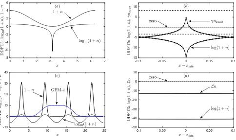
at the points in spacexbetween the density peaks, where
the density is a minimum. On increasing the average den-sity beyond this point in the phase diagram, there is no solution to the theory. We analyse in detail this singu-lar behaviour. Asρ(x)→0 we have logρ(x)→ −∞, of
course. In the equation for the equilibrium density profile this divergence is initially balanced by the term involving the fourth derivative, ∂4ρ/∂x4 → +∞. However, when the average density in the system is increased beyond the value at which this divergence occurs, we find there is no solution.
We illustrate these conclusions by finding the pre-dicted structures and phase diagram for the 2D version of the GEM-4 (Generalised Exponential Model of index 4) [41, 42], chosen because DDFT based on a simple ap-proximation (the so-called random phase apap-proximation (RPA) [43]) for the Helmholtz free energy functional can be very accurate for predicting the equilibrium struc-tures formed in this model and also the thermodynam-ics [42, 44, 45]. At higher temperatures, the 2D GEM-4 system exhibits just a single fluid phase and at higher densities a single crystal phase. At lower temperatures, where the RPA DDFT is no longer accurate, there is a hexatic phase and multiple crystalline phases as the density is increased [42]. Here we do not consider this regime, restricting ourselves to the regime where there is just one fluid and one crystal phase, which are predicted accurately by the RPA DDFT. This enables us to inves-tigate the effect of making subsequent approximations to the DDFT, including those made to derive PFC theory. We find that the PFC type theories spuriously predict three additional phases that are in reality not present in the phase diagram (i.e., are not thermodynamically stable). These are (i) a stripe phase, (ii) what we refer to as ‘down hexagons’ (in contrast to the true crystal structure, which we refer to as ‘up hexagons’) and then at even higher densities a melting to form (iii) another uniform liquid phase. We show how the approximations made in deriving the PFC result in these structures being predicted.
The final contribution of this paper is to show that there is a very simple and accurate ansatz one can make for the form of the equilibrium crystal density profile in DDFT (and so also for DFT, of course). The ansatz is ρ(x) =ρ0eφ(x), where ρ0 is a constant and the field
φ(x) is approximated by a sinusoid of the formφ(x)≈
φ0+φ1eik·x+complex conjugate (in one dimension), plus other similar terms (in higher dimensions), whereφ0and φ1 are constants. The results presented here are for the GEM-4 model and show why this approximation is un-expectedly accurate: the approximation is able to repli-cate almost exactly the numerical solution to the DDFT problem, from small to arbitrarily large amplitude den-sity variations. We expect this ansatz also to be reliable for other systems. This form of one-mode theory gives a hint for future directions to develop accurate PFC-type theories, since using a one-mode approximation in PFC is often fairly accurate.
This paper is structured as follows: In Sec. II we present our systematic step-by-step derivation of PFC, starting from DDFT. After each approximation, we care-fully state the model, i.e., we give the corresponding free energy functional and also the expression for the chemi-cal potential, which is a quantity that is a constant at all points in space for equilibrium states. In order to keep track of the different orders in which the approximations can be made, we give each model a name, starting with PFC-αfor the original PFC model in Eq. (2) above, and with DDFT-0 for the original formulation of DDFT be-low. The different DDFT approximations result in five different versions, DDFT-1 to DDFT-5. Similarly, we explain the various different approximations that can be made to each of these, leading to a corresponding PFC theory, which we name PFC-αto PFC-ǫ. Note that the criterion we use here for distinguishing between whether we refer to a theory as a DDFT or a PFC is based on whether the free energy which is minimised by the dy-namical equations (i.e., the Lyapunov functional) has the logarithmic ideal gas term or not: if it does not have the logarithm, we refer to it as a PFC. Table I below is there to help the reader navigate the various models and the approximations made in each one. Sec. II concludes with a summarising discussion. In Sec. III we present results for the GEM-4 system comparing predictions for the density profiles and thermodynamics of equilibria for two of the different DDFT theories and also two of the PFC theories. In this section we also present the phase diagrams for the GEM-4 system predicted by these dif-ferent DDFT and PFC theories. By comparing all of these we are able to assess the accuracy of the different theories and the validity of the various approximations. In Sec. IV we discuss the implications of the main two approximations and analyse the singular behaviour dis-played by some models. In Sec. V we introduce the ansatz ρ(x) =ρ0eφ(x)and derive the new one-mode approxima-tion for DDFT. We draw our conclusions in Sec. VI. The paper includes two appendices in which we describe the numerical (continuation) methods we use to calculate the density profiles.
II. DERIVATION OF THE PHASE FIELD CRYSTAL MODEL FROM DDFT
re-sults in PFC-β, from DDFT-3 results in PFC-γ, and so on up to PFC-ǫ. The PFC-ǫmodel can be rescaled to recover the original version of PFC, PFC-α, see Eqs. (1) and (2). The various models are summarised in Table I. Amongst the models we present below, DDFT-5 is equivalent to the model derived by Huanget al.[24] and advocated by van Teeffelenet al.[23] (named PFC1 in that paper), and DDFT-3 and PFC-ǫare equivalent to the models named DDFT and PFC2 by van Teeffelenet al.[23].
A. Dynamic Density Functional Theory: DDFT-0
The starting point for all of our derivations is the key DDFT equation [28–31]:
∂ρ ∂t =∇ ·
βM(ρ)∇δδρF
, (5)
where β = (kBT)−1 (with kB being Boltzmann’s
con-stant andT being temperature),M(ρ) is the positiveρ -dependent mobility. The Helmholtz free energyF[ρ] de-pends on the density profileρ(x, t) integrated over space;
henceF[ρ] depends on time but not on position [30]. The expression δF/δρis the functional derivative of F with respect toρ(x, t), which therefore depends on both time
and on position. DDFT usually takes M(ρ) =Dρ, i.e., the mobility is proportional to density [28–31], whereDis the diffusion coefficient. We henceforth scale time so that D= 1. With boundary conditions that do not allow ma-terial to enter or leave the system, N = R
ρ(x)dx (or
equivalently, the mean density) is a constant of the mo-tion and is the total number of particles in the system.
With suitable boundary conditions, one can readily show that the Helmholtz free energy decreases monoton-ically with time:
dF
dt =−
Z
βM(ρ)
∇
δF
δρ
2
dx≤0, (6)
so (assuming that F[ρ] is bounded below) the system typically evolves to a (local) minimum of F, which is a dynamically stable equilibrium of (5). Here, ‘dy-namically stable’ means that small perturbations away from the equilibrium decay, and ‘equilibrium’ means that ∂ρ/∂t= 0 and dF/dt = 0. Owing to the dynamics be-ing governed by a continuity equation (4), such pertur-bations cannot change the mean density. Local minima of F that are not the global minimum are thermody-namically metastable. The system can also have dynam-ically unstable equilibria, for whichFis a saddle or max-imum. From (6), we see that all equilibria of (5) satisfy
∇(δF/δρ) = 0, so
δF
δρ = constant =µ, (7)
whereµis the chemical potential of the equilibrium. This is of course the Euler–Lagrange equation for the problem
of finding stationary points of the functionalF[ρ], subject to the constraint of fixed mean density. Note however that when evolving (5) forward in time from an arbitrary initial condition,µis not necessarily known a priori.
The theory can also be cast in terms of the grand potential (also called the Landau free energy) func-tional [25–27]:
Ω[ρ] =F[ρ]−µN =F[ρ]−µ
Z
ρ(x)dx. (8)
From this it follows that the functional derivative of Ω is δΩ
δρ = δF
δρ −µ, (9) and that this is zero at equilibrium: equilibria are ex-treme values of Ω. Like the Helmholtz free energy, the grand potential decreases monotonically with time, since Eq. (6) is also true if one replacesFby Ω. Therefore, for two phases to coexist, they must have the same specific grand potential (i.e., the same pressure) and the same chemical potential. Thus, the global minimum of Ω for a givenµandT is the thermodynamic equilibrium state of the system [25–27].
Following the usual approach in DFT, we separate the Helmholtz free energy into three parts: the ‘ideal gas’ contribution, which is proportional to the temperature but takes no account of particle interactions, an excess (Fex) over the ideal gas contribution arising from the par-ticle interactions, and the contribution due to an external potentialUext(x), as follows [25–27]:
F[ρ] =kBT Z
ρ log(Λdρ)−1
dx+Fex[ρ] + Z
ρUextdx,
(10) where the integral is taken over the volume V in three dimensions (d= 3) (or the area in 2D,d= 2) and where Λ is the thermal de Broglie wavelength. Since for our purposes here the value of Λ is irrelevant (changing Λ will shift the values ofF andµby constants), we henceforth set Λ = 1. We also consider bulk systems and so we assume thatUext = 0. With the separation in Eq. (10), we have
βδF
δρ = logρ+β δFex
δρ , (11) which gives
β∇δδρF =1
ρ∇ρ+. . . , (12) where on the right hand side we only explicitly write the contribution from the ideal gas part of the free energy. Inserting this into Eq. (5) withM =Dρwe obtain
∂ρ ∂t =∇
2ρ+. . . , (13)
in which the coefficient in front of the term∇2ρisD, but our choice of time scaling hasD= 1. Note that this term islinear in ρ, in spite of it originating from a nonlinear
logarithmic contribution to the free energy.
Name Truncate atO(c(4))
LDA (31) for
c(3) andc(4)
RY/RPA:
c(3)=c(4)= 0
Gradient expansion
ofL(44)
Constant mobility,
expand log(1 +n) Dynamics Free energy
Chemical
potential Q,C,R
PFC-α Yes N/A Yes Yes Yes (2) (1) — Q= 0
C=−1
DDFT-0 (5) (10) (7) —
DDFT-1 Yes (24), (26) (25) (28), (30) —
DDFT-2 Yes Yes (34) (32) (36) (35)
DDFT-3 Yes N/A Yes (41) (40) (42)
Q=12
C= 0
R= 0
DDFT-4 Yes N/A Yes (46) as (32) as (36) (35)
DDFT-5 Yes N/A Yes Yes (48) (47) (49)
Q=1 2
C= 0
R= 0
PFC-β Yes Yes Yes (53), (54) (52) (55) (56)
PFC-γ Yes N/A Yes Yes (58) (57) (59) Q=
1 2
C=−13
PFC-δ Yes N/A Yes Yes as (54) as (52) as (55) (56)
PFC-ǫ Yes N/A Yes Yes Yes (60) as (57) as (59) Q=
1 2
[image:6.595.57.560.56.355.2]C=−13
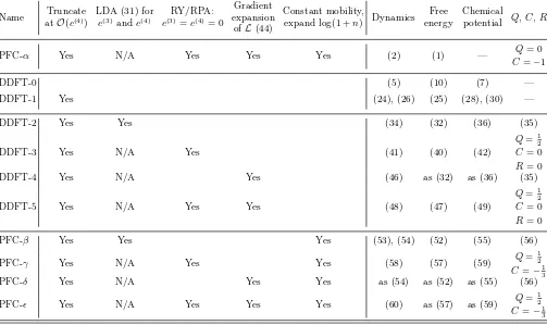
Table I: Various versions of DDFT and PFC, in order of appearance, along with references to the equations defining the dynamics, the free energy and the chemical potential. We also give the quadratic (Q), cubic (C) and quartic (R) coefficients. PFC-αis the phenomenological model, also known as the conserved Swift–Hohenberg equation; PFC-ǫis equivalent to PFC-α.
B. Expansion of Fex: DDFT-1
To proceed, we must have an expression for the excess Helmholtz free energy functionalFex[ρ]. We use a func-tional Taylor expansion, which is also that used in all derivations of PFC theory. This gives the free energy functional of the system of interest in terms of prop-erties of a reference system, which are assumed to be known. The reference system that is chosen is a uniform liquid, with constant density ρ0. The density profile of the system of interest may be varying in space and with an average density that may be different from ρ0. The functional Taylor series expansion of the excess free en-ergy can be written in terms of the density difference ∆ρ(x, t) =ρ(x, t)−ρ0 as follows [26, 27]:
Fex[ρ] =Fex[ρ0]−kBT Z
c(1)(x1)∆ρ(x1)dx1
−kBT
2!
Z
c(2)(x
1,x2)∆ρ(x1)∆ρ(x2)dx1dx2
−kB3!T Z
c(3)(x1,x2,x3)×
∆ρ(x1)∆ρ(x2)∆ρ(x3)dx1dx2dx3
+ similar fourth order term +. . . .
(14)
The expressions c(n) in the equation above are propor-tional to the first and higher funcpropor-tional derivatives ofFex with respect to density, all evaluated atρ=ρ0:
c(n)(x1, . . . ,xn) =−β δ nF
ex
δρ(x1). . . δρ(xn)[ρ0]. (15)
These functionsc(n)are known asdirect correlation
func-tions[25–27], and are related ton-point density correla-tion funccorrela-tions. In the two-point case, c(2) is the pair direct correlation function and is related to the pair cor-relation function (i.e., the radial distribution function) through the Ornstein–Zernike equation [25–27]. These direct correlation functions depend on our choice of ρ0 and depend directly on temperature through the linear factor ofβ in the definition (15) and also indirectly via the fact that the correlations in a liquid change with tem-perature. Note also thatc(1)[ρ
0] is a constant whenρ0is a constant.
For a homogeneous liquid with distant (or periodic) boundaries, these functions depend on displacements but not on absolute position, so (through a slight abuse of notation) we also write
c(n)(x1, . . . ,xn) =c(n)(∆x2,∆x3. . . ,∆xn), (16)
where ∆xj=xj−x1[27]. We also take the liquid to be
We are considering density perturbations away from the liquid state, so it is convenient to write
ρ(x, t) =ρ0(1 +n(x, t)). (17)
We do not assume thatnis small, but it is often the case that the average ofn(x, t) over the whole system is small.
Note also thatρ(x, t) =ρ0is a stationary solution of (5).
Substituting Eq. (14) into Eq. (5) and writing only the terms up toc(1), we get:
∂n ∂t =∇
2n
− ∇2c(1)− ∇ ·hn∇c(1)i+. . . (18)
That the uniform liquid state is an equilibrium of (5) implies that n = 0 is a solution of equation (18): all terms not written down involve ∆ρ and so are zero for the uniform liquid with density ρ0. Recall that c(1)[ρ0] is a constant, which means terms involving gradients of this can be dropped. Whilst this constant term does not influence the structure (density profile) both in and out of equilibrium, it does affect the thermodynamics (i.e., free energy value) and so also mechanical properties [46]. With this, we can write the equation for the time evolu-tion ofn(x, t) (up to O(c(4))) as:
∂n ∂t =∇
2n
−ρ0∇2
Z
c(2)(x,x2)n(x2)dx2
−ρ0∇ ·
n∇ Z
c(2)(x,x2)n(x2)dx2
−ρ
2 0 2 ∇
2Z c(3)(x,x
2,x3)n(x2)n(x3)dx2dx3
−ρ
2 0 2 ∇ ·
n∇ Z
c(3)(x,x2,x3)n(x2)n(x3)dx2dx3
−ρ
3 0 6 ∇
2Z c(4)(x,x
2,x3,x4)×
n(x2)n(x3)n(x4)dx2dx3dx4
−ρ
3 0 6 ∇ ·
n∇ Z
c(4)(x,x2,x3,x4)×
n(x2)n(x3)n(x4)dx2dx3dx4
+. . .
(19)
where we have suppressed writing the time dependence of n throughout and the x dependence of n when it is
not inside an integral. We have written this equation so that the first line is linear in n, the next two lines are quadratic inn, the fourth and fifth lines are cubic in n, and the last line is quartic inn.
Since the first line is linear inn, and both terms involve a Laplacian, we can write the linearised version of (19) in terms of the negative Laplacian of a linear operatorL:
∂n ∂t =−∇
2
Ln, (20)
where
Ln(x) =−n(x) +ρ0 Z
c(2)(x,x2)n(x2)dx2. (21)
k k2σ(k)
[image:7.595.334.545.54.148.2]k= 1
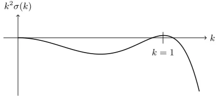
Figure 1: Illustrative example of the growth rate k2σ(k) as a function of wavenumber k. Small amplitude modes with
k2σ(k) < 0 decay exponentially in time, while those with
k2σ(k)>0 grow exponentially. Throughout we scale lengths so that the maximum growth rate occurs atk= 1.
The non-local operatorLis most conveniently considered in terms of its Fourier transform, or equivalently, in terms of how it acts on modes of the form exp(ik·x). If
Leik·x
=σ(k)eik·x, (22)
then σ(k) is the eigenvalue of L with eigenfunction
exp(ik·x). With this, the linear equation (20) can
read-ily be solved in terms of linear combinations of functions like exp k2σ(k)t+ik·x
, where k2σ(k) is the growth rate for a mode with wavevectork, and k=|k|. Ifσ(k)
is negative for allk, all small amplitude density
modu-lations decay to zero, and the liquid state is dynamically stable.
Recall that for a bulk liquid, c(2)(x,x
2) =c(2)(∆x2), with ∆x2 = x2 − x, and for spherically symmetric
(isotropic) particles, c(2)(x,x
2) = c(2)(|∆x2|). There-fore, in this case σ(k) = σ(k), i.e., σ depends only on
the wavenumber k = |k|. The eigenvalue σ(k) can be
expressed as:
σ(k) =−1 +ρ0
Z
c(2)(|x2−x|)eik·(x2−x)
dx2
=−1 +ρ0ˆc(2)(k),
(23)
function [27]. So, for the stable uniform liquid, we have σ(k) =−1/S(k).
We refer to the state point at which the uniform liquid becomes linearly unstable to density modulations with wavenumber k 6= 0 as the spinodal point, in keeping with the terminology of [48]. The more common usage of the term ‘spinodal’ relates to the onset of the zero-wavenumber phase separation instability of liquid–liquid or gas–liquid phase separation [27, 30]. At the spinodal point, the density and temperature are such that the liq-uid is dynamically marginally stable, that is, the max-imum of k2σ(k) is zero. Therefore, at higher tempera-tures, small amplitude density modulations decay, and at lower temperatures, small amplitude density modula-tions grow. For a given fixed value of ρ0, the spinodal temperature isTs, with a correspondingβs= (kBTs)−1.
Similarly, either increasing the density ρ0 of the liquid or increasing the chemical potential µ can also lead to crossing the spinodal.
With (21), we can eliminatec(2)in favour ofLin (19), and obtain (truncating atO(c(4))):
∂n ∂t =− ∇
2
Ln+12n2
− ∇ ·[n∇Ln]
−ρ
2 0 2 ∇
2Z c(3)(x,x
2,x3)n(x2)n(x3)dx2dx3
−ρ
2 0 2 ∇ ·
n∇ Z
c(3)(x,x2,x3)n(x2)n(x3)dx2dx3
−ρ
3 0 6 ∇
2Z c(4)(x,x
2,x3,x4)×
n(x2)n(x3)n(x4)dx2dx3dx4
−ρ
3 0 6 ∇ ·
n∇ Z
c(4)(x,x2,x3,x4)×
n(x2)n(x3)n(x4)dx2dx3dx4
(24)
where we have used the result∇·[n∇n] = 12∇2n2. For an ideal gas, withLn=−nand c(2) =c(3) =c(4) = 0, the first line of the equation above reduces to the diffusion equation, ∂n∂t =∇2n, similar to (13).
At this point, we have made no approximations be-yond expanding the free energy in Eq. (14) and trun-cating at O(c(4)). We refer to the model at this stage, truncated in this way, as DDFT-1. In the new variables, and incorporatingc(2) intoL, the Helmholtz free energy
F can be expressed (up to fourth order) in terms of a
scaled free energyF1=F/ρ0, where
βF1[n] =
Z
[1 +n(x1)] log[1 +n(x1)]−n(x1)dx1
−12 Z
n2(x1) +n(x1)Ln(x1)
dx1
−ρ
2 0 6
Z
c(3)(x1,x2,x3)×
n(x1)n(x2)n(x3)dx1dx2dx3
−ρ
3 0 24
Z
c(4)(x1,x2,x3,x4)×
n(x1)n(x2)n(x3)n(x4)dx1dx2dx3dx4,
(25)
and where we have also dropped terms that do not con-tribute to (24). In these variables, the DDFT that leads to the dynamics (24) is
∂n ∂t =∇ ·
β(1 +n)∇δF1
δn
. (26)
Note that, because of the log(1 +n) term in (25), n is constrained so that 1 +n is always non-negative. Also, because of Eq. (17), we have
δF
δρ = δF1
δn . (27)
Moreover, states that satisfy
δF1
δn = ∆µ, (28)
where ∆µ=µ−µ0 and where [see (7), (10) and (14)]
µ0=kBTlog Λdρ0−kBT c(1)[ρ0], (29)
are equilibrium solutions of (24), or equivalently, extrema of F1. Henceforth, we redefine µ to be β∆µ/ρ0, which is a shifted and rescaled chemical potential. For the free energy in (25), we have
βδF1
δn = log (1 +n(x))−n(x)− Ln(x)
−ρ
2 0 2
Z
c(3)(x,x2,x3)n(x2)n(x3)dx2dx3
−ρ
3 0 6
Z
c(4)(x,x2,x3,x4)×
n(x2)n(x3)n(x4)dx2dx3dx4.
(30)
C. Simplification of c(3) and c(4): DDFT-2
As the next step, Huanget al.[24] kept only the zero-wavenumber components ofc(3) andc(4), or equivalently, they took
c(3)(x,x2,x3) =c(3)
0 δ(x−x2)δ(x−x3),
c(4)(x,x2,x3,x4) =c(4)
0 δ(x−x2)δ(x−x3)δ(x−x4), (31)
wherec(3)0 andc (4)
0 are constants (our sign convention is opposite to that of [24]). This is equivalent to making a local density approximation (LDA) [26] for these terms in the free energy. We could in principle include terms involvingc(5)and higher as well, treated in the same way: these would contribute a more general function ofnin the free energy, treated with the LDA. However, since we are investigating the effect of approximations that have not yet been discussed, we keep as simple a free energy as pos-sible at this point, consistent with truncating atO(c(4)). With this, the free energy in (25) becomes
βF2[n] =
Z
[1 +n(x)] log[1 +n(x)]−n(x)
dx
+
Z
−12 n2(x) +nLn(x)
−ρ
2 0 6 c
(3)
0 n3(x)− ρ3
0 24c
(4) 0 n4(x)
dx,
(32)
and the four terms involvingc(3) andc(4)in (24) become
−ρ
2 0 2 c
(3)
0 ∇2n2, − ρ2
0 2c
(3) 0 ∇ ·
n∇n2
, −ρ 3 0 6 c (4)
0 ∇2n3 and − ρ3
0 6c
(4) 0 ∇ ·
n∇n3
.
(33)
Using ∇ ·
n∇n2
= 23∇2n3 and ∇ ·
n∇n3
= 34∇2n4, Huanget al.[24] combined (33) and (24) to get
∂n ∂t =−∇
2
Ln+Qn2+Cn3+Rn4
−∇·[n∇Ln] (34)
where
Q= 1 2+
ρ2 0 2c
(3) 0 , C=
ρ2 0 3 c (3) 0 + ρ3 0 6c (4)
0 and R=
ρ3 0 8c (4) 0 . (35) We also have a chemical potential
µ=βδF2
δn = log (1 +n(x))−n(x)− Ln(x)
−ρ
2 0 2 c
(3)
0 n2(x)− ρ3
0 6c
(4) 0 n3(x),
(36)
which does not vary in space at equilibrium. Up to this point, we refer to the model as DDFT-2.
Here, we retain then4term (as did Huang et al.[24]), because otherwise the dynamics in (34) would not be
consistent with the free energy (32) and the DDFT dy-namics (26) (withF2instead ofF1).
The next three models involve making (or not mak-ing) two approximations: (i) assuming the Ramakrishan– Yussouff or random phase approximation, which leads to a quadratic excess Helmholtz free energy functional, and (ii) making a gradient expansion of the linear operatorL.
D. Quadratic excess free energy: DDFT-3
Often, the free energy functional in (14) is truncated atO(∆ρ2). This is known as the Ramakrishan–Yussouff (RY) approximation [7, 23, 49], which effectively sets c(3) = c(4) = 0. A mathematically equivalent approx-imation arises in the treatment of soft purely repulsive particles modelling soft matter, namely the RPA [43]. Here, two soft isotropic particles atx1 andx2 separated
by a distancex12=|x1−x2|interact through a potential energyu(x12), which depends only on the magnitude of the distance and is finite for all values ofx12. The excess free energy [c.f. Eq. (14)] is then
Fex[ρ] = 1 2
Z
u(|x1−x2|)ρ(x1)ρ(x2)dx1dx2. (37)
This amounts to settingc(3)=c(4)= 0 and
c(2)(x1,x2) =−βu(|x1−x2|) (38)
in DDFT-2. The eigenvaluesσ(k) can thus be related to the Fourier transform ofuthrough (23) [5, 43]:
σ(k) =−1−ρ0β
Z
u(|x−x2|)eik·(x2−x)dx
2
=−1−ρ0βuˆ(k).
(39)
Setting c(3) = c(4) = 0 implies from (35) that Q = 1 2, C= 0 and R= 0, and results in a free energy
βF3[n] =
Z
(1 +n(x1)) log(1 +n(x1))−n(x1)
dx1
−12 Z
n2(x1) +n(x1)Ln(x1)dx1.
(40)
With this choice of free energy, the dynamics in (34) be-comes:
∂n ∂t =−∇
2
Ln+12n2
− ∇ ·[n∇Ln], (41)
along with an analogous version of (36), for the chemical potential:
µ=βδF3
δn = log (1 +n(x))−n(x)− Ln(x) (42)
Before moving on to make further approximations, it is worth noting a useful property that DDFT-3 and the subsequent theories derived from it possess. If the pair potential u(x12) in Eq. (38) can be written asu(x12) = ǫψ(x12), where ǫ is a parameter that controls the over-all strength of the potential, then from Eqs. (21), (38) and (42) we obtain:
µ= log (1 +n(x)) +ρ0βǫ Z
ψ(|x−x2|)n(x2)dx2. (43)
The consequence of this is that for a given ψ, the be-haviour of the model depends only on the combination of parameters ρ0βǫ and the value of µ. If one changes the value of the reference densityρ0to some other value, then this is entirely equivalent to solving the system with the original reference densityρ0at a different value ofβǫ. We should emphasize that this is only true ifψ does not change with density, which in general is not true, but is approximately the case for some systems.
E. Gradient expansion of the linear term: DDFT-4
Returning to DDFT-2, Huanget al.[24] (following [2]) expanded L in powers of the gradient operator ∇, re-placing L by the simplest linear operator that allows a positive growth rate for modes with a wavenumber ks.
Scaling lengths so thatks= 1 results in:
Lgradn=rn−γ(1 +∇2)2n, (44)
soσ(k) =r−γ(1−k2)2from (22). This approximation is equivalent (within scaling) to a local gradient expansion of (21), expanding the Fourier transform ofc(2) about its maximum:
ρ0cˆ(2)(k) = 1 +r−γ(1−k2)2, (45)
where the function ρ0ˆc(2)(k) and its second derivative evaluated at k = 1 are 1 +r and −8γ, respectively. Here,ris a parameter, notionally increasing withβ (and with ρ0) and equal to zero at the spinodal point, when β=βs. This parameter controls the growth rate of waves
with wavenumber 1: effectively, r is the height of the maximum at k = 1 in the growth rate curve in Fig. 1. The second parameterγ can be used to fit the curvature of ˆc(2)(k) atk= 1.
With this gradient expansion, the dynamics is
∂n ∂t =−∇
2 L
gradn+Qn2+Cn3+Rn4
− ∇ ·[n∇Lgradn].
(46)
We refer to this model as DDFT-4: Lgradis now a (local) partial differential operator and (46) is a partial differ-ential equation. The free energy and chemical potdiffer-ential can be found from (32) and (36), settingL=Lgrad. The lower bound n ≥ −1 is still respected. This model is equivalent to that written down by [24].
Higher powers (or other functions) of the Laplacian can be retained inLgrad, to improve the accuracy of the match between the eigenvalues of L and Lgrad, as done for example by [9, 10], or to introduce additional unstable length scales, as done for example by [11–14] and others. See also Eq. (76) below and the associated discussion.
F. RY and gradient expansion: DDFT-5
Finally, we can make both the RY/RPA approxima-tion (c(3)0 =c(4) = 0) and replace the linear operator L by Lgrad to get the model advocated in Ref. [23]. The free energy and evolution equation are
βF5[n] =
Z
(1 +n(x1)) log(1 +n(x1))−n(x1)
dx1
−1
2
Z
n2(x1) +n(x1)Lgradn(x1)
dx1,
(47)
and
∂n ∂t =−∇
2
Lgradn+12n2− ∇ ·[n∇Lgradn], (48)
along with an analogous version of Eq. (42) for the chem-ical potential:
µ=βδF5
δn = log (1 +n(x))−n(x)− Lgradn(x) (49)
This model is named PFC1 in [23], but here we call it DDFT-5 for consistency.
G. PFC models
The final simplification that can be made (or not made) is to discard the ∇ ·[n∇Ln] (or ∇ ·[n∇Lgradn]) term from the dynamical equations for the four DDFT els DDFT-2, . . . , DDFT-5, resulting in four PFC mod-els PFC-β, . . . , PFC-ǫ. Huang et al.[24] justify making this simplification on the grounds that this term is not truly quadratic inn: the presence ofLnin the expression means that it is effectively of higher order. However, we show below that this term does in fact make an important contribution to the free energy: at least as important as thec(3) term.
cancels the ρ−1, leading to a diffusion equation in (13). If the ∇ ·[n∇Ln] term is dropped from (34), the equa-tion for n becomes of the form ∂n
∂t = ∇
2δG
δn for some
functional G[n]. We can see the implications of this by returning to (5) and taking the steps needed to get to this modified version of (34). Clearly the mobility in (5) has been taken to be constant. If we now think of the ideal gas part of the free energy in (10) and (11), but with a constant mobility in the dynamical equation, we end up with the ideal gas term contribution to the equation forρ being the form
∂ρ ∂t =
1 ρ∇
2ρ− 1 ρ2|∇ρ|
2
(50)
instead of the diffusion equation (13). This unlikely equa-tion can be avoided, and the diffusion equaequa-tion recovered at leading order, by expanding the logarithm in (32) in a Taylor series. Thus, dropping the ∇ ·[n∇Ln] term is equivalent to taking constant mobility and expanding the logarithm.
It is because of these substantial changes that we opt to use the term ‘DDFT’ for all models based on free energies that have the logarithmic ideal gas term, the non-constant mobility and the∇ ·[n∇Ln] term retained. In contrast, we use the term ‘PFC’ for models based on expanding the logarithm, having a constant mobil-ity and the∇ ·[n∇Ln] term dropped. One consequence of expanding the logarithm up to O(n4), as is done in most PFC derivations [7], is that the ideal gas part of the free energy contributes cubic and quartic (as well as quadratic) terms to the free energy, so going from DDFT-2 to PFC-β turns out not to be just a matter of dropping the∇ ·[n∇Ln] term.
So, a consistent free energy–dynamics derivation [2, 23] involves going back to DDFT-2 and replacing the logarithm in (32) by:
(1 +n) log(1 +n) =n+12n2−16n 3+ 1
12n
4, (51)
resulting in a free energy
βFβ[n] =
Z
−1 2nLn−
1 6n
3+ 1 12n 4 −ρ 2 0 6 c (3) 0 n3−
ρ3 0 24c
(4) 0 n4
dx1,
(52)
where we have suppressed writing the x1 dependency
of n(x1). Taking the mobility M(ρ) in (5) to be a
con-stant (M =Dρ0) implies (after scaling)
∂n ∂t =∇
2βδFβ δn
, (53)
similar to (2). This leads to the PFC dynamical equation:
∂n ∂t =−∇
2
Ln+Qn2+Cn3
(54)
and to a chemical potential
µ=βδFβ
δn =−Ln−Qn 2
−Cn3, (55)
whereQis as in (35) butC is different:
Q=1 2 +
ρ20 2 c
(3)
0 and C=−
1 3 +
ρ30 6 c
(4)
0 . (56)
We refer to this model as PFC-β, and recall that the factor ofβ in front ofFβ is the inverse temperature.
The end result here is that PFC-β (54) is not the same as DDFT-2 (34) with the∇ ·[n∇Ln] term removed: the cubic coefficientC is different and the quartic contribu-tionRn4 in (34) is absent. For the cubic coefficient, the contribution proportional toc(3)0 in (35) comes from the non-constant mobility, while the−1
3 term in (56) comes from expanding the logarithm. The contribution to C proportional to c(4)0 is the same. Moreover, the 1
2 in Q in (35) and (56), while having the same numerical value, arises for two different reasons: non-constant mobility versus expanding the logarithm. An additional differ-ence between the DDFT and PFC models is that in the PFC models, the constraint thatn≥ −1 (i.e.,ρ≥0) is not enforced.
As in the DDFT derivations, we can now make (or not make) the RY/RPA approximation and the gradient ex-pansion. We consider first the RY/RPA approximation, settingc(3)=c(4) = 0 in PFC-β. The free energy is
βFγ[n] =
Z −1
2nLn− 1 6n
3+ 1 12n
4
dx1, (57)
the dynamics is
∂n ∂t =−∇
2 Ln+1
2n 2−1
3n 3
(58)
and the chemical potential is
µ=βδFγ
δn =−Ln− 1 2n
2+1 3n
3. (59)
We refer to this model as PFC-γ, and it is effectively the same as PFC-β but withQ= 12 andC=−13.
Finally, the gradient expansion can be made, re-placing L by Lgrad in all expressions in this subsec-tion, resulting in PFC-δ (without RY/RPA) and PFC-ǫ (with RY/RPA).
We refer to these models collectively as the PFC mod-els, and have chosen the names PFC-αetc. to distinguish these from the PFC1 and PFC2 models of Ref. [23]. The quadratic term in the dynamics (Qn2) can be removed (providedC 6= 0) by adding a constant ton(x), but we
choose not to do this as it implies a change to what was meant byρ0 in the reference liquid. In addition, a nega-tiveC can be scaled to−1. With these changes, PFC-ǫ is equivalent to the original PFC-αmodel (2) of [1, 2]:
∂n ∂t =−∇
2 rn
−γ(1 +∇2)2n+Qn2+Cn3
, (60)
where we have written outLgrad explicitly, and Q = 12 and C = −1
and adding a constant ton– returning to the conserved Swift–Hohenberg equation).
The implication of dropping the∇·[n∇Ln] term in the dynamics (41) for DDFT-3 is now apparent: without this term, Eq. (41) reduces to (58) but with the cubic term removed. The absence of the cubic term here implies a free energy as in (57) that is not bounded below, i.e., a free energy that is non-physical, and so the ∇ ·[n∇Ln] term can have the effect of stabilizing patterns. In ad-dition, dropping the ∇ ·[n∇Ln] term is consistent only with a theory with a constant mobility.
H. Summary
To summarise, we have carefully laid out the vari-ous approximations made in the progression from the DDFT-0 starting point (5) to the final PFC (2,58) writ-ten down in [1, 2]. We have largely followed earlier deriva-tions [7, 23, 24], seeking to clarify the approximaderiva-tions that are made. Along the way, we have identified four intermediate versions of DDFT, listed for clarity in Ta-ble I. The change in name from DDFT to PFC could be made at any point in this progression, but we prefer to make the name change at the point where the∇·[n∇Ln] term is dropped (along with all the other changes that are implied by this), since removing this term marks a considerable alteration to the free energy expression and to the dynamics.
The PFC model (54) is appealing in its simplicity, and it gives insight into a variety of crystallisation phenom-ena, but the derivations of the model from DDFT pre-sented here, as well as the derivation from Ref. [24], are both problematic. Just dropping the∇ ·[n∇Ln] term, as done by Huanget al.[24], means that the dynamics is not equivalent to a DDFT with mobility proportional to ρ. On the other hand, the alternative is to expand the loga-rithm up toO(n4) in (51) in order to provide anonlinear stabilizing term (121n4) in the free energy (57). However, in the original formulation, the logarithm comes from the ideal gas term in (10), and leads to alinear diffusive term in the dynamics. The stabilizing nonlinear terms in (34) are provided byc(3)0 ,c
(4)
0 (in DDFT-2) and by the
∇ ·[n∇Ln] term – these are all absent in PFC-γ. Indeed, all these models only make physical sense if their free energies are bounded below. The free ener-gies for DDFT-0 and DDFT-1 are too general to make any comment, but that for DDFT-2 (32) etc. can be dis-cussed. The (1 +n) log(1 +n)−nterm is bounded below by zero, and the−1
2
R
nLndxterm is bounded below
be-cause the eigenvalues ofLare bounded above:
− Z
n(x)Ln(x)dx≥ −σmax Z
n2(x)dx, (61)
where σmax is the maximum over k ofσ(k) (we have in mind aσ(k) as in Fig. 1). In any case, this term, along with the other quadratic and cubic terms, is dominated by the quartic in n, which is bounded below provided
c(4)0 <0. Ifc (4)
0 = 0, then c (3)
0 <0 will do, recalling that n≥ −1. For DDFT-3, with the RY/RPA approximation c(3)0 =c(4) = 0, the boundedness of the free energy (40) depends on the n2+nLn combination. From (21), the relevant term is
− Z
n2(x1) +n(x1)Ln(x1)dx1=
−ρ0
Z
n(x1)c(2)(x1,x2)n(x2)dx1dx2.
(62)
In general, this is not bounded below, but it is in certain circumstances. For example, it is ifσmax<−1, and it is ifc(2)(x
1,x2)≤0 (or u(|x1−x2|)≥0 for RPA) for all
x1 andx2, which is the case in the numerical examples
below. The PFC models are not constrained to have n≥ −1, butFβ (52) is bounded by then4 term as long as its coefficient is positive; Fγ (57) is always bounded below, because the expansion of the logarithm in (51) was truncated after an even powered term.
Throughout we have made the simplest choices in the approximations, but other authors have made many other choices. For example, the original PFC paper [1], as well as later papers [22, 24, 50–52], included a two-component (binary) version of the PFC model. Recently, Wanget al.[53] took a much closer look atc(3) andc(4), expressing these in terms of isotropic tensors and so al-lowing these functions to introduce bond angle depen-dence into the free energy. Some choices ofc(3) and c(4) lead to nonlinear terms that include gradients, which can affect the selection of the final stable crystal [54]. The gradient expansion approach has been generalised in two ways: (i) higher order terms or rational functions were considered by [9, 10] in order to improve the fit between the functional form and the Fourier transform of c(2), and (ii) PFC models with two unstable length scales have been put forward by several authors [10–15], since these allow more complex crystals (face-centered cubic, icosa-hedral quasicrystals, . . . ) to be stabilized. We discuss the model of [9] in more detail below. Alternative approaches involving weighted densities are also possible [55].
III. COMPARISON OF DDFT AND PFC
We are interested in the effects of the approximations made in going from DDFT to PFC. A full assessment of the validity of the RY/RPA approximation forFex, which in itself constitutes a major simplification, is beyond the scope of the present study. The general conclusion on the validity of the RY/RPA approximation is that it depends on the nature of the interactions between the particles; there are examples in the literature where this approxi-mation is reliable and others where it works badly – see for example the discussion in Refs [56, 57] and references therein.
approximating L by Lgrad and of making the suite of other approximations inherent in going from DDFT to PFC: expanding the logarithm, assuming constant mo-bility and dropping the∇ ·[n∇Ln] term. To this end, we start with DDFT-3 and solve (42), rewritten here as:
DDFT-3: log (1 +n(x))−n(x)− Ln(x) =µ. (63)
The system that we consider is particles interacting via the GEM-4 [41, 42] potential: this is a model for soft-matter particles and in particular for dendrimers and other polymers in suspension, treating the polymers via an effective pair potential between their centers of mass. This potential is soft, i.e., finite for all values ofx12[41– 43, 58, 59], and is
u(x12) =ǫe−(x12/R)
4
, (64)
where the parameter ǫ controls the strength of the po-tential andRcontrols its spatial range. We consider here the system in 2D [42, 45]. As long as the temperature and density are high enough that the particle cores reg-ularly overlap (the regime in which the system freezes), the RPA approximation (37) is known to be rather ac-curate for the GEM-4 system and gives a good account of the phase diagram and the structure of the liquid and solid phases [42, 44, 45].
From Eqs. (21), (38) and (64) we obtain the linear operatorL:
Ln(x) =−n(x)−ρ0βǫ Z
e−|x−x2| 4
/R4
n(x2)dx2. (65)
Recall from (22) thatLhas eigenvaluesσ(k) with eigen-functions eik·x
. We can choose the combined parameter ρ0βǫ and soft-particle radiusRso that the maximum in σ(k) occurs atk= 1 when the system is at the linear sta-bility threshold, i.e., this is a maximum with σ(1) = 0, similar to Fig. 1. In 2D, to satisfy this condition we must have ρ0βǫ = 0.2455 and R = 5.0962 – see Appendix A for details.
With this choice of parameters, the eigenvalueσ(k) is shown as a solid line in Fig. 2. The figure also shows (dashed line) the eigenvalue for the gradient expansion ofLaroundk= 1:
Lgradn(x) =−γ(1 +∇2)2n(x), (66)
whereγ= 4.37 is chosen to match the second derivative d2
σ
dk2 at k = 1, as done for example in Refs. [2, 9, 60].
The dotted line in Fig. 2 is the eigenvalue for (76), the eighth-order fitting model proposed in [9] and discussed in more detail below.
In what follows we compare solutions of (63) for DDFT-3 with solutions of the analogous equations for DDFT-5, PFC-γ and PFC-ǫ:
DDFT-5: log (1 +n)−n− Lgradn=µ, (67) PFC-γ: −12n
2+1 3n
3
− Ln=µ, (68) PFC-ǫ: −12n
2+1 3n
3
− Lgradn=µ. (69)
0 0.5 1 1.5 2
[image:13.595.325.545.56.192.2]-20 -15 -10 -5 0
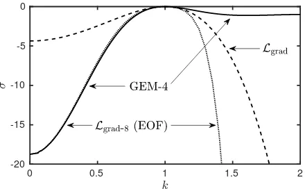
Figure 2: The eigenvalueσ(k) ofLplotted as a function of wavenumberk for the GEM-4 potential (solid line) forR= 5.0962 andρ0βǫ= 0.2455, which is at the threshold where the system becomes linearly unstable. This hasσ(0) =−18.75. We also displayσ(k) from the gradient expansion ofL(dashed line), i.e., a Taylor expansion in Fourier space aroundk= 1, which is the PFC relation forLgrad,σ(k) =−γ(1−k2)2, with
γ= 4.37. Recall that the growth rate of Fourier modes with wavenumberk is isk2σ(k). The dotted line labelledL
grad-8 (EOF) is the curve for (76), the eighth-order fitting proposed in [9]: it nearly coincides with the GEM-4 curve fork≤1.
See Appendix B for details of the pseudo-arclength con-tinuation numerical method we use for solving these equations. Also, in the supplementary material we in-clude a Matlab code for solving DDFT-3. Note that throughout what follows, we refer to the quantity 1+n(x)
as the ‘density’.
Since the DDFT-5, PFC-γand PFC-ǫrepresent differ-ent forms of Taylor expansion around the reference state with densityρ0, there are a variety of ways comparison between solutions can be made. Here, we opt to fix L
and Lgrad as in (65) and (66) with the specified values of ρ0βǫ, R and γ. This implies that at µ = 0 the ref-erence state with n = 0 is at the spinodal point and is marginally unstable to modes with wavenumberk = 1. We then vary µstarting from µ= 0 and follow the liq-uid, stripe and hexagonal solutions of (63) and (67)–(69) in appropriately sized two-dimensional domains. For a given value ofµthe different solutions have different val-ues for the mean density 1 + ¯n= 1 +A1R
n(x)dx, where
Ais the area of the domain. For each state we calculate the specific grand potential:
Ω[n] A =
F[n]
A −µ(1 + ¯n), (70)
where F is F3, F5, Fγ or Fǫ, as appropriate. We also
-5 0 5 10 0
1 2 3
-5 0 5 10
-20 -15 -10 -5 0 5
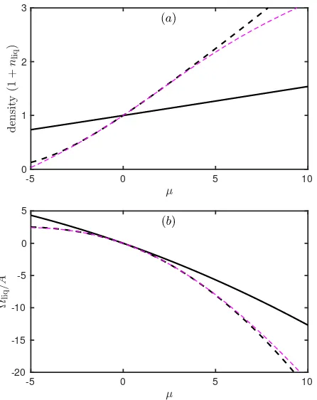
Figure 3: (a) Liquid density (1 +nliq) and (b) specific grand potential Ωliq/Aas a function of the scaled chemical potential
µ, for DDFT-3 (solid black line), DDFT-5 (dashed black line), PFC-γ(indistinguishable from DDFT-3) and PFC-ǫ(dashed magenta line).
equilibria might result from initial conditions via the dy-namics.
The solution corresponding to the uniform density liq-uid state with n(x) =nliq can readily be found. In this
case we haveLnliq=σ(0)nliq, and so we must solve the following algebraic equations fornliq:
DDFT-3,5: log (1 +nliq)−nliq−σ(0)nliq=µ, (71) PFC-γ,ǫ: −1
2n 2 liq+13n
3
liq−σ(0)nliq=µ, (72)
recalling that the value of σ(0) depends on whether or not the gradient expansion is carried out (see Fig. 2). Finding nliq for a given value of µ is done easily using Newton’s method, and the resultingnliq and specific Ωliq are shown in Fig. 3. In all cases, we see that nliq is an increasing function of µ, while Ωliq/A is a decreas-ing function of µ. The figure shows that the specific grand potential for the liquid state predicted by all four models are similar close toµ= 0, but the predicted liq-uid state densities are rather different away fromµ= 0. This difference originates from the different values ofσ(0) (−18.75 for DDFT-3 and PFC-γ, in contrast to −4.37 for DDFT-5 and PFC-ǫ). We see from Fig. 3 that the density of the liquid is erroneously predicted to increase too rapidly asµ is increased by the gradient expansion
theories (DDFT-5 and PFC-ǫ). This is because these get the value of the isothermal compressibilityχT to be
too large [9]. This compressibility is related toσ(0) via χT =−β/[σ(0)ρ0(1 +nliq)] [27]: see Eq. (23) and follow-ing discussion. Expandfollow-ing the logarithm makes relatively little difference over this range of densities.
Since crystallisation occurs at higher densities, we ex-pect a transition from the liquid to the crystal to occur as µ increases. At the spinodal the uniform liquid be-comes linearly unstable and the patterned state solution branches bifurcate from the liquid at this point. To find these states, we seek a solution of the form
n(x) =nliq+δn(x), (73)
where near the bifurcation pointδn≪1, andδnis of the formeik·x
, so thatLδn=σ(k)δn. Expanding Eqs. (63) and (67–69) in powers ofδnwe find that theO(1) equa-tions to solve are just those for finding the liquid state density, Eqs. (71)–(72). TheO(δn) equations are
DDFT-3,5:
1
1 +nliq −
1−σ(k)
δn= 0, (74)
PFC-γ,ǫ: −nliq+n2liq−σ(k)
δn= 0. (75)
The spinodal point for DDFT-3,5 or for PFC-γ,ǫis where there are solutions of the equation withδn6= 0.
Since we are looking for a change in stability, we take the extreme value of σ(k), i.e., σ(k) = 0 (see Fig. 2). Then, Eq. (74) is solved (withδn6= 0) only fornliq= 0, which leads toµ= 0 from (71). In contrast, Eq. (75) with σ(k) = 0 has two solutions,nliq= 0 andnliq= 1, leading toµ= 0 and µ=−1
6−σ(0) from (72). The implication of this is that the PFC has two spinodal points: the liq-uid loses stability at nliq = 0 as µ increases through 0, but it regains stability atnliq= 1, which givesµ= 18.58 for PFC-γandµ= 4.20 for PFC-ǫ. This prediction that the liquid regains stability for higherµis a consequence of expanding the logarithm, or equivalently of Taylor ex-panding the 1/(1 +nliq) term in (74) and is confirmed by direct computation of the crystal solutions below. Of course, this prediction is erroneous, since the simulation results for the GEM-4 system [41, 42] show no sign of a second spinodal point or the associated stable second liquid in the equilibrium system phase diagram.
[image:14.595.62.285.55.336.2]10 20 30 40 50
0.5 1 1.5 2 2.5 3
1 2 3 4 5
-4 -3 -2 -1 0 1
-0.5 0 0.5
[image:15.595.67.559.54.261.2]-1 -0.5 0 0.5
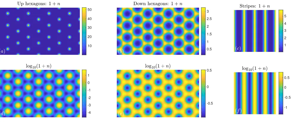
Figure 4: Examples of solutions of DDFT-3 (63) withµ = 10. (a,d) Up hexagons (isolated density maxima surrounded by density that is small but positive) in a 8π×√8
3 wavelength domain, with 2.3×10
−5 <1 +n < 52.3. (b,e) Down hexagons
(isolated density minima) in a 8×√8
3 wavelength domain, with 0.12<1 +n <3.3. (c,f) Stripes in a 4×4 wavelength domain, with 0.045<1 +n <5.9. The top row (a–c) shows the density 1 +nand the bottom row (d–f) shows log10(1 +n).
it is possible to go a bit higher in µ, but with increas-ing µ (i.e., increasing average density) the peaks in the density profile get narrower and higher and so more and more grid points are required to resolve these peaks cor-rectly. However, as we show below for some of the other models and for different reasons, it is not possible to con-tinue the solutions this far inµ. The domains on which the profiles are calculated have periodic boundary condi-tions, with 4 wavelengths in each direction (for stripes), or 8×√8
3 wavelengths (for hexagons). The wavelength is initially equal to 2πforµ= 0 and is then adjusted by up to about 2% in order to minimise the specific grand po-tential asµis varied; i.e., we minimise Ω/Awith respect to variations in the size of the crystal unit cell or, for the stripe phase, we minimise with respect to variations in the spacing between the stripes – see Appendix B for details.
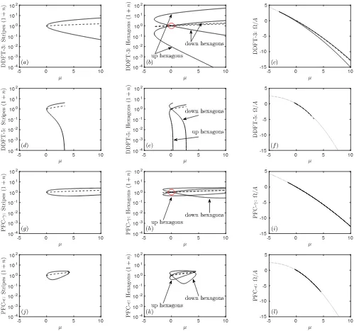
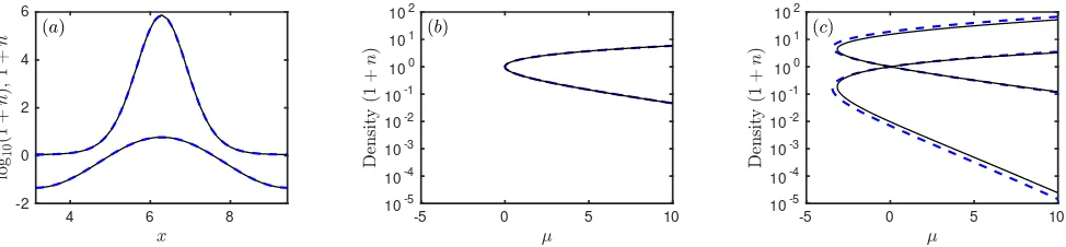
In Fig. 5 we display a series of plots showing the maxi-mum, minimum and average values of the density profiles 1+nfor the stripe and hexagonal structures as a function ofµ. We also plot the specific grand potential Ω/Afor the different structures. Recall that for a given µthe ther-modynamic equilibrium phase corresponds to the global minimum of Ω/A. The results for DDFT-3 are shown in Fig. 5(a–c). The (a) stripes originate in a supercrit-ical pitchfork bifurcation at µ = 0, and (b) hexagons originate in a transcritical bifurcation at the same value ofµ. The density of the up hexagons ranges from about 2×10⁻⁵up to about 50, forµ= 10. All of these branches can be continued to larger values ofµ.
DDFT-5, in Fig. 5(d–f), initially behaves in the same
way, but all three branches have their minimum density heading to zero before µ gets to 10: this happens at µ≈3.37 for (d) stripes, and forµ≈0.28 andµ≈2.73 for (e) the up and down branches of hexagons, respectively. The numerical method cannot continue the branches be-yond these points. We argue in Sec. IV that this is not an artefact of the numerical method, rather it is a genuine feature of solutions of Eq. (67) that the density 1 +n can go to zero. In this limit, log(1 +n)→ −∞, but this is balanced by a lack of smoothness inn(x): the fourth
derivative in Lgradn can go to +∞ and so balance the singularity in log(1 +n). Therefore,µ≈0.28 is the limit of validity of the DDFT-5 model.
The two PFC examples are similar to each other, and it is easier to discuss PFC-ǫ, in Fig. 5(j–l), first. Here, (j) stripes and (k) hexagons bifurcate from the liquid at µ= 0, but they rejoin the liquid atµ= 4.20 as explained in the discussion following Eqs. (74–75). The maximum and minimum densities for the up and down hexagon cross between the two bifurcations. The behaviour of PFC-γ, in Fig. 5(g–i), is similar, though the second bi-furcation is atµ= 18.58, off the scale of the figure.
-5 0 5 10 10-4
10-3 10-2 10-1 100 101 102
-5 0 5 10
10-4 10-3 10-2 10-1 100 101 102
-5 0 5 10
-15 -10 -5 0 5
-5 0 5 10
10-4 10-3 10-2 10-1 100 101 102
-5 0 5 10
10-4 10-3 10-2 10-1 100 101 102
-5 0 5 10
-15 -10 -5 0 5
-5 0 5 10
10-4 10-3 10-2 10-1 100 101 102
-5 0 5 10
10-4 10-3 10-2 10-1 100 101 102
-5 0 5 10
-15 -10 -5 0 5
-5 0 5 10
10-4 10-3 10-2 10-1 100 101 102
-5 0 5 10
10-4 10-3 10-2 10-1 100 101 102
-5 0 5 10
[image:16.595.54.553.85.552.2]-15 -10 -5 0 5