Integrated comparative validation tests as an aid for building simulation tool users and developers

Integrated Comparative Validation

Tests as an Aid for Building

Simulation Tool Users and

Developers

5

6

ABSTRACT 7

Published validation tests developed within major research projects have been an invaluable aid to 8

program developers to check on their programs. This paper sets out how selected ASHRAE Standard 140-9

2004 and European CEN Standards validation tests have been incorporated into the ESP-r simulation 10

program so that they can be easily run by users, and discusses some of the issues associated with 11

compliance checking. Embedding the tests within a simulation program allows program developers to 12

check routinely whether updates to the simulation program have led to significant changes in predictions 13

and to run sensitivity tests to check on the impact of alternative algorithms. Importantly, it also allows 14

other users to undertake the tests to check that their installation is correct and to give them, and their 15

clients, confidence in results. This paper also argues that validation tests should characterize some of the 16

significant heat transfer processes (particularly internal surface convection) in a greater level of detail in 17

order to reduce the acceptance bands for program predictions. This approach is preferred to one in which 18

validation tests are overly prescriptive (e.g. specifying fixed internal convection coefficients) as these do 19

not reflect how programs are used in practice. 20

INTRODUCTION 21

Validation has been a part of program development from the beginning of the development of thermal 22

simulation programs and thus there is a long history of its application. Through experience, a consensus 23

has been reached on the various elements of the validation process (for example, Judkoff et al 1983, Jensen 24

1993, and Bloomfield 1999). These comprise the following: 25

• Review of theory 26

• Code checking 27

• Analytical verification 28

• Inter-program comparison 29

• Empirical validation 30

The first two of these are necessary for any technical software development. To permit future 31

developments and re-use, high quality comprehensive documentation of the theory and its implementation 32

is an essential element for state-of-the-art programs which are too complex for individuals to develop. The 33

advantages and disadvantages of the other three techniques are well understood, as is the fact that all 34

techniques need to be applied on a regular basis during program development. 35

The ESP-r program (ESRU 2005) has been the subject of numerous validation studies over a period of 36

almost three decades. A summary of all the main validation studies is given by Strachan et al (2005). They 37

comprise studies included as part of European projects, within several IEA Annexes/Tasks, within national 38

studies and as part of PhD theses. It was observed that the early exercises were mostly focussed on 39

empirical validation as this is the most obvious method to test program validity. However, these early 40

studies indicated the difficulties with experimental studies – the need for high levels of instrumentation, 41

consideration of all heat and mass flow paths/processes, accurate control and minimisation of uncertainty. 42

Following this, a more balanced view was taken which emphasised the complementary nature of the 43

various validation techniques. 44

IEA Annex 21/Task 12 Co-operative Project. This comprehensive study (Judkoff and Neymark 1

1995, Lomas et al 1994) was concerned with analytical verification (testing for steady state and dynamic 2

conduction, the incidence of direct solar radiation on external surfaces of arbitrary orientation, and the 3

transmission of direct radiation through simple glazing systems), inter-program comparisons (development 4

of BESTEST, focussed on passive solar spaces involving a diagnostic method – this was based on 5

incremental changes to a base case model with comparisons between predictions from a number of detailed 6

public domain programs) and empirical validation based on data from test rooms (using detailed monitored 7

data from two small outdoor test cells). The work extended from 1988 to 1993 and involved many person-8

years of effort: for example, predictions from 17 programs were included in the empirical validation 9

exercise. 10

PASSYS. This European project was concerned with the establishment of outdoor test cells. Part of the 11

work was conducted by a model validation group (Jensen 1993), who undertook detailed analysis of the 12

ESP-r program including a review of algorithms, inter-program comparison, analytical verification and 13

sensitivity studies. A number of detailed empirical validation studies were also conducted. Again, this was 14

a large project, extending from 1986 to 1993 and involving a number of research groups throughout 15

Europe. 16

IEA Annex 43/Task 34 Co-operative Project. This project, started in 2004, intends to extend the 17

work of IEA Annex 21/Task 12. It will focus on more complex tests involving, amongst others, multi-zone 18

heat and mass transfer, double facades and the interactions between shading, lighting and loads. Teams 19

from countries in Europe, North America and Japan are involved. 20

Although only a few of the larger studies are highlighted above, it is clear that significant resources are 21

required to undertake thorough validation. And in spite of such multi-year, multi-team projects, there are 22

numerous areas of program functionality that have not yet been fully tested. 23

A key observation from this large range of studies is that the validation tests are not persistent. By this 24

it is meant that, although the program may have achieved reasonable agreement with measured data in 25

empirical studies, or other programs in comparative studies, there is no certainty that this level of 26

agreement is achieved several years later. For example, the original ranges obtained in the IEA Annex 27

21/Task 12 BESTEST qualification tests which have been adopted in ASHRAE Standard 140 28

(ANSI/ASHRAE 2004) were all obtained from simulations run with a number of programs about 12 years 29

ago. There have been innumerable program developments and bug fixes in the intervening period, and as 30

shown in a later section in this paper, program predictions have changed. This is the underlying reason why 31

it is considered necessary to embed the tests and regularly monitor them to check if there have been 32

significant changes in predictions. There is also a clear need for regular review of published ranges. 33

Embedding the tests to enable their easy application, particularly those tests in approved Standards, is 34

also of benefit to program users concerned with validation and accreditation. Program developers are often 35

asked by those who directly use the simulation program or those who commission simulation-based design 36

appraisals regarding the confidence that can be placed in results and whether the program has been 37

validated. Including the tests with the program allows users to check compliance with Standards for 38

themselves, as well as confirming that the program has been properly installed. It is becoming increasingly 39

important that programs are shown to comply with national and international Standards, and embedding the 40

tests in the simulation program allows the check to be made easily by users, and possibly, in the future, by 41

those in charge of program accreditation. 42

This paper sets out the facility developed within ESP-r and discusses the ASHRAE and CEN 43

validation tests that have been incorporated into the structure. Results from the ASHRAE fabric and 44

envelope tests and the CEN summer overheating tests are presented, highlighting some modelling issues. 45

Two sensitivity studies are then described, involving changing the solar algorithm and the internal 46

convection algorithm, to demonstrate how the embedded tests can be used to investigate the impact of code 47

changes and to show how significant these choices are. Finally, conclusions are drawn and 48

recommendations made for future work. 49

FRAMEWORK FOR EMBEDDED VALIDATION 50

Ben-Nakhi and Aasem (2002) developed a set of solutions for dynamic heat transfer through opaque 51

multi-layer constructions involving a step change in internal or external temperatures. Constructional 52

thermophysical properties can be defined by the user, together with the inside and outside boundary 53

simulation period and simulation timesteps can be specified. Predictions from a thermal simulation 1

program can be compared to the analytical solution. 2

What was novel about the work was that it was implemented within a simulation program (ESP-r). 3

After the user specifies the input data listed above, a thermal zone is automatically created, a simulation 4

performed and results extracted for comparison with the analytical solution. It is therefore straightforward 5

to undertake the tests at regular intervals during program development, or to check on numerical accuracy 6

and stability for any particular construction. Ben-Nakhi and Aasem set out the structure for embedding 7

other validation checks and it is this structure which has been extended in the work reported here. 8

A significant recent development in energy simulation has been the inclusion of validation tests within 9

standards, reflecting the increasing move towards performance-based standards instead of prescriptive 10

standards. Of note are the adoption of the BESTEST comparative tests within ASHRAE Standard 140, 11

mentioned in the previous section, and the inclusion of validation tests in proposed CEN European 12

Standards (at present, those concerned with summer overheating and cooling load calculations). There are 13

some differences in approach between the ASHRAE and CEN Standards. The ASHRAE Standard 140 is 14

less prescriptive in specifying simulation parameters. The specified ranges of predictions for particular tests 15

are sometimes large, reflecting the different assumptions and algorithms used by the various programs 16

involved in the range setting. On the other hand, the CEN Standards are more prescriptive, for example by 17

specifying the surface coefficients that should be used, and for this reason narrower tolerance bands are 18

specified. 19

To demonstrate the usefulness of embedding validation tests, comparative tests from the ASHRAE 20

Standard 140 that focus on the building thermal envelope and fabric loads, and from the CEN Standard 21

13791 (CEN 2004) that focus on summer overheating risk, have been included in the ESP-r program. It was 22

intended that they were implemented so that they can be easily run by program developers and users. 23

ASHRAE Standard 140 Building Thermal Envelope and Fabric Load Tests 24

The ASHRAE tests are grouped into high mass and low mass cases, and classed as either basic 25

sensitivity tests or in-depth sensitivity tests. The tests are designed so that it is primarily the differences 26

between pairs of tests that are of interest: for example, the difference in prediction between two models 27

which are identical apart from a change in the external surface absorptivity. There is also a group with four 28

free float tests and one test which has a second free float zone. Results are also presented in the Standard 29

from all the individual models. 30

The basic sensitivity tests analyse the ability of software to model building envelope loads by varying 31

the window orientation, shading devices, set-back thermostat and night ventilation. The in-depth sensitivity 32

tests 195 through 320 analyse the ability of software to model building envelope loads for a non-deadband 33

on/off thermostat control configuration with the following variations among the cases: no windows, opaque 34

windows, exterior infra-red emittance, infiltration, internal gains, exterior shortwave absorptance, south 35

solar gains, interior shortwave absorptance, window orientation, shading devices, and thermostat setpoints. 36

In-depth cases 395 through 440, 800 and 810 analyse the ability of software to model building envelope 37

loads in a deadband thermostat control configuration with the following variations: no windows, opaque 38

windows, infiltration, internal gains, exterior shortwave absorptance, south solar gains, interior shortwave 39

absorptance, and thermal mass. 40

Using ESP-r, the user can access the tests where they have the choice to run a specific group of tests, 41

run individual tests or run all the tests. After selecting the models to be run, simulation is automatically 42

invoked with pre-defined parameters without the need for user intervention. For every simulation, results 43

analysis is also automatically invoked and the specific results for every test are recovered and saved in a 44

file. In order to know what kind of results need to be recovered for each case, a recovery data file which is 45

provided with each of the models is read in. 46

Apart from the free float tests, for every case selected in the groups, the files with the recovered results 47

are scanned and the differences in the peak and annual heating and cooling loads are extracted. The results 48

can be displayed or sent to an external file. 49

In addition to the simulation results, the minimum and maximum limits listed in the ASHRAE 50

Standard 140 informative annexes are displayed to the user. A check is made whether or not the recovered 51

results are within the specified range and an "outside" or "inside" message is given to notify the user. (It is 52

worth noting that ASHRAE Standard 140 is a standard method of test and not a pass/fail standard.) 53

Another set of predictions is also displayed. This could be from the previous released version of the 54

As the tests are designed to separately stress most of the fundamental heat transfer processes, this is a 1

useful diagnostic tool. Alternatively, it is possible to display the ESP-r predictions originally obtained in the 2

IEA Annex 21 project which are published in the ASHRAE Standard 140, so that the magnitude of changes 3

over the last 12 years can be quantified. These are the values presented in this paper. 4

The same approach applies to the free float and the individual tests. For the free float tests, the files 5

with the recovered results are scanned for the minimum and maximum temperatures together with the time 6

of occurrence and the annual average temperature. For all the other individual tests, the results are scanned 7

for the peak heating and cooling loads, their time of occurrence and also for the annual heating and cooling 8

loads. Some tests require more specific data to be extracted (either annual or hourly for a specific date). 9

This additional data requirement is also specified in the results recovery data files, so that it can be 10

extracted and presented to the user. 11

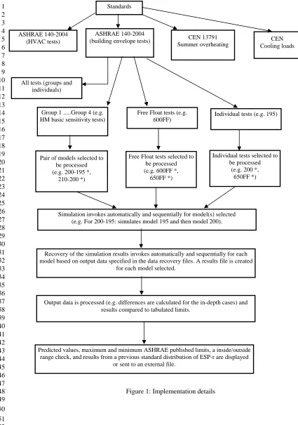
Figure 1 sets out the overall structure of the implemented approach. 12

CEN Standard 13791: Calculation of room temperatures in summer without mechanical 13

cooling 14

The CEN (European Standards Organisation) is currently producing a series of standards on 15

calculation methods for the design and the evaluation of the thermal performance of buildings and building 16

components. In this area, proposed Standard 13791:2004 (CEN 2004) is at the formal vote stage, whereby 17

its implementation is imminent. The process of certification in Europe is based on defining a standard 18

method to solve the problem and a performance based approach to certification. This process allows 19

developers to either adopt the standard equations and solution process for compliance, or using their own 20

equations prove that they are within the acceptable range of the published data. In the case of CEN 21

Standard 13791:2004 the recommended approach is that of solving the governing equations using an 22

implicit finite difference approach. 23

The CEN standard tests are implemented in a similar manner to the ASHRAE tests described above. 24

Within proposed Standard 13791, four areas of the simulation tool’s performance are examined in separate 25

tests. These tests are: 26

1. Transient response in a solid opaque construction to a 10˚C change in external temperature. This test 27

examines the transient conduction algorithm in isolation as all other aspects of the model are fixed 28

(radiation and convection coefficients). 29

2. Internal long-wave radiation under steady state conditions, given boundary temperatures and a solar 30

gain to a surface. 31

3. Solar shading to examine the ability of a program to calculate the degree of shading of direct solar 32

radiation for six shading device configurations, over a period of several hours. 33

4. An overall whole model test to examine the combined modelling of solar, conduction and internal 34

radiation modelling for two single zone geometries. There are no shading devices in these tests, but 35

there are heat gains from casual sources and ventilation air flows. 36

The proposed CEN Standard 13791 is specific in its application – a single zone model without 37

mechanical heating or cooling for a warm period. It does not apply to spaces where solar can pass through, 38

or which are adjacent to a sunspace or atrium, for which a more robust model would be required. The tests 39

examine the software's ability to model the main thermal flow paths in buildings where there is no 40

mechanical system. 41

The proposed Standard is prescriptive in specifying many aspects of the heat transfer processes. In 42

some cases, these differ from how the processes are modelled in existing simulation programs. In the case 43

of ESP-r, differences in modelling approaches were found in the handling of solar distribution, convective 44

heat transfer coefficients, boundary condition specification and room air thermal capacity. Thus changes 45

needed to be made at source code level to conform with the requirements of the proposed Standard (for 46

example, allowing a new adiabatic boundary condition with exactly the same specification as that in the 47

Standard). This type of intervention can be done only by program developers or other experienced users. 48

Also, some of the required outputs were not available directly from the results module (which is needed for 49

automatic recovery of results without user intervention for embedded tests): it was necessary to undertake 50

The specific validation tests, described below in more detail with results obtained, have been placed in 1

the same structure as described above for the ASHRAE Standard 140 fabric and envelope tests. Again there 2

are tolerance bands given in the Standard against which predictions can be compared, and it is possible to 3

detect whether there have been changes in prediction from a previous application of the tests. 4

RESULTS FROM IMPLEMENTATION OF ASHRAE STANDARD 140 5

It is not intended to give a complete set of results in this paper due to space constraints, so just one 6

typical example from each category is given in Table 1. The table shows the results obtained from using the 7

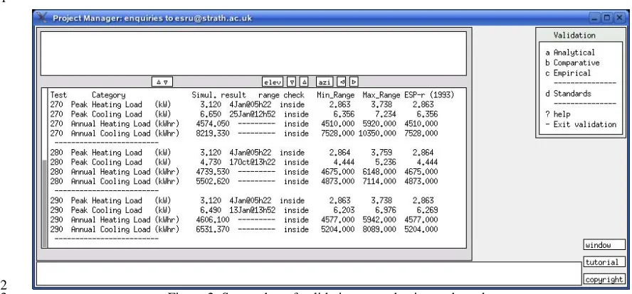
new embedded models. Figure 2 is a screenshot to show how results are presented to the user, which can 8

also be redirected to a file. The table shows the test number, the output parameter, the predicted result, the 9

inside/outside range check against the range given in the informative annexes of the ASHRAE Standard, 10

the range limits, and finally the results from the runs carried out in IEA Annex 21 by De Montfort 11

University using ESP-r in 1993. The internal convection algorithm is known to cause significant 12

uncertainty in predictions (see later section in this paper). Therefore, these runs were done with the same 13

internal convection algorithm as used in the IEA Annex 21 BESTEST simulations. This enables an 14

evaluation to be made of the impact of other program changes over the last 12 years. 15

In Table 1: 16

• 910-900 is a "High mass basic sensitivity test" which tests south overhang/mass interaction (the 17

difference between models 910 and 900). 18

• 610-600 is a "Low mass basic sensitivity test" which tests the effect of a south overhang (the 19

difference between models 610 and 600). 20

• 900-810 is a "High mass basic and in-depth sensitivity test" which tests interior solar absorptance 21

and mass interaction (the difference between models 900 and 810). 22

• 270-220 is a "Low mass in-depth sensitivity test" which tests south solar transmittance/incidence 23

solar radiation (the difference between models 270 and 200). 24

• 650FF is a "Free float test" which tests venting of a free floating room. 25

• 410 is an "Individual test" which tests infiltration. 26

27

TABLE 1 28

Results from selected ASHRAE 140 fabric and envelope tests 29

Test Category

ESP-r

(2005) CHECK

Min Range

Max

Range ESP-r (1993)

910-900 Peak Heating Load (kW) 0.010 inside 0.003 0.019 0.008

910-900 Peak Cooling Load (kW) -0.590 inside -1.122 -0.310 -0.992

910-900 Annual Heating Load (kWh) 207 inside 179 442 405

910-900 Annual Cooling Load (kWh) -1142 inside -1561 -832 -1311

610-600 Peak Heating Load (kW) 0.000 inside -0.011 0.001 0.000

610-600 Peak Cooling Load (kW) -0.590 inside -0.811 -0.116 -0.525

610-600 Annual Heating Load (kWh) 33 inside 21 98 59

610-600 Annual Cooling Load (kWh) -1702 inside -2227 -1272 -2222

900-810 Peak Heating Load (kW) -0.130 inside -0.166 -0.089 -0.129

900-810 Peak Cooling Load (kW) 1.060 inside 0.595 1.223 1.036

900-810 Annual Heating Load (kWh) -658 outside -1107 -669 -669

900-810 Annual Cooling Load (kWh) 1209 inside 975 1707 1080

270-220 Peak Heating Load (kW) -0.010 inside -0.034 0.218 -0.004

270-220 Peak Cooling Load (kW) 5.870 inside 5.475 5.894 5.796

270-220 Annual Heating Load (kWh) -2418 inside -2761 -1948 -2434

270-220 Annual Cooling Load (kWh) 7951 inside 7342 9515 7342

650FF Annual Hourly Max Temp (˚C) 66.4 inside 63.2 68.2 63.2

650FF Annual Hourly Aver Temp (˚C) 18.9 inside 18.0 19.6 18.2

410 Peak Heating Load (kW) 3.880 inside 3.625 4.487 3.625

410 Peak Cooling Load (kW) 0.310 inside 0.035 0.814 0.035

410 Annual Heating Load (kWh) 8620 inside 8596 10506 8596

410 Annual Cooling Load (kWh) 11 inside 0 84 0

1

The following points were noticed in the results obtained. 2

a) There are, in some cases, significant differences in the current results from predictions obtained in the 3

IEA Annex 21 work and those from the current version of ESP-r. There have been many code 4

developments and bug fixes in the intervening years. Of particular note are updates in the solar 5

algorithms (e.g. updates to some of the solar equations, including a change of algorithm for the 6

anisotropic diffuse sky to use of the Perez (1990) model). This is investigated in a later Section of this 7

paper. 8

b) There is now an occasional “outside” recorded, with one example given in Table 1. In some cases in 9

the range setting in the IEA Annex 21 work, ESP-r predictions formed either the lower or higher limits 10

of the identified range. Due to changes in the code, sometimes the predictions have changed to be 11

outside the specified range. It is usually by a small amount, but nevertheless, may be of interest 12

because it indicates that there may be a greater degree of variability between programs for this test than 13

currently indicated in the informative annex to the ASHRAE Standard 140. It also underlines the need 14

for the regular updating of the informative annex. 15

RESULTS FROM IMPLEMENTATION OF CEN STANDARD 13791 16

Tables 2 to 6 show how simulation results for prediction of air temperatures, sunlit factors and 17

operative temperatures compare against the test limits in the forthcoming Standard. 18

19

TABLE 2 20

Results of CEN13791 conduction tests (air temperatures, ˚C) 21

Time (hrs)

Test 1 Test 2 Test 3 Test 4

Low High ESP-r Low High ESP-r Low High ESP-r Low High ESP-r

2 19.56 20.56 20.04 24.59 25.59 24.67 19.50 20.50 20.00 19.50 20.50 19.98

6 20.76 21.76 21.29 29.13 30.13 29.50 19.76 20.76 20.25 19.56 20.56 20.04

12 22.98 23.98 23.46 29.50 30.50 29.98 21.17 22.17 21.64 19.75 20.75 20.23

24 25.87 26.87 26.36 29.50 30.50 30.00 24.40 25.40 24.85 20.13 21.13 20.61

120 29.50 30.50 29.96 29.50 30.50 30.00 29.45 30.45 29.94 22.67 23.67 23.15 22

Table 2 shows a comparison between predictions and Standard 13791 results for the opaque 23

conduction test. The test comprises four separate constructions subjected to a 10˚C change in external 24

temperature. For each test the lower and upper acceptable air temperatures are given for the required times 25

after the step change in external temperature. To implement the test no source code changes were 26

necessary and the convective heat transfer coefficients had to be specified (overriding the system default). 27

As can be seen, predictions lie within the limits prescribed for this test. 28

29

TABLE 3 30

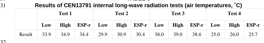
Results of CEN13791 internal long-wave radiation tests (air temperatures, ˚C) 31

Test 1 Test 2 Test 3 Test 4

Low High ESP-r Low High ESP-r Low High ESP-r Low High ESP-r

Table 3 shows the internal air temperature in each of the four zone configurations for the long-wave 1

radiation test. Again, no source code modifications were necessary and for these tests only the convection 2

coefficients were changed from the default approach adopted by ESP-r, with the solar gain to the single 3

surface modelled as a controlled flux to that surface (it is not possible to have a solar gain in a zone 4

comprising only opaque surfaces). As can be seen, predictions are within the required limits for this long-5

wave radiation test. 6

7

TABLE 4 8

Results of CEN13791 direct solar shading tests (sunlit factor, -) 9

Time (hrs)

Test 1 Test 2 Test 3 Test 4 Test 5 Test 6

Low High ESP-r

Low High ESP-r

Low High ESP-r

Low High ESP-r

Low High ESP-r

Low High ESP-r

7 0.00 0.05 0.00 0.00 0.05 0.00 0.00 0.05 0.00 0.00 0.05 0.00 0.95 1.00 1.00 0.00 0.05 0.00

8 0.48 0.58 0.50 0.42 0.52 0.49 0.00 0.05 0.00 0.95 1.00 1.00 0.84 0.94 0.87 0.00 0.05 0.00

9 0.19 0.29 0.23 0.71 0.81 0.77 0.00 0.50 0.00 0.95 1.00 1.00 0.66 0.76 0.73 0.02 0.12 0.07

10 0.16 0.26 0.21 0.92 1.00 0.98 0.13 0.23 0.19 0.95 1.00 1.00 0.34 0.44 0.40 0.67 0.77 0.73

11 0.25 0.35 0.30 0.95 1.00 1.00 0.25 0.35 0.33 0.85 0.95 0.87 0.00 0.05 0.03 0.95 1.00 1.00

12 0.28 0.38 0.35 0.95 1.00 1.00 0.28 0.38 0.33 0.79 0.89 0.80 0.00 0.05 0.00 0.95 1.00 1.00 10

Table 4 shows the sunlit factor for the test surface for each of the six configurations of shading device. 11

The test specifies the solar location for each of the calculation times. It is not possible to explicitly set the 12

solar position in ESP-r (it is a function of the site location and time). It was discovered by an iterative 13

approach that the site location was 52˚N and 0.5˚W of the local time meridian for the 15th of June (the 14

latitude and date were set in an earlier draft of the standard). The result for test 6 at 12 noon requires the 15

solar shading to be calculated for a solar azimuth of 180˚ (due south) – this is parallel to the east-facing test 16

surface, so it could be argued that the surface is neither in shade nor direct sunlight (although the test 17

assumes that this is fully sunlit). As can be seen, the results are within the published ranges and thus 18

comply with the solar shading test. 19

20

TABLE 5 21

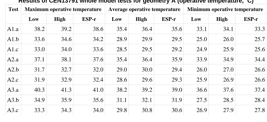
Results of CEN13791 whole model tests for geometry A (operative temperature, ˚C) 22

Test Maximum operative temperature Average operative temperature Minimum operative temperature

Low High ESP-r Low High ESP-r Low High ESP-r

A1.a 38.2 39.2 38.6 35.4 36.4 35.6 33.1 34.1 33.3

A1.b 33.6 34.6 34.2 28.9 29.9 29.5 25.0 26.0 25.7

A1.c 33.0 34.0 33.6 28.5 29.5 29.2 24.9 25.9 25.6

A2.a 37.1 38.1 37.6 35.4 36.4 35.9 33.9 34.9 34.4

A2.b 31.7 32.7 32.0 29.0 30.0 29.4 26.0 27.0 26.6

A2.c 31.9 32.9 32.4 28.6 29.6 29.3 25.9 26.9 26.6

A3.a 40.3 41.3 41.0 38.2 39.2 39.0 36.6 37.6 37.4

A3.b 34.9 35.9 35.6 31.1 32.1 31.9 27.5 28.5 28.4

A3.c 33.3 34.3 34.0 29.8 30.8 30.6 26.9 27.9 27.8

1

TABLE 6 2

Results of CEN13791 whole model tests for geometry B (operative temperature, ˚C) 3

Test Maximum operative temperature Average operative temperature Minimum operative temperature

Low High ESP-r Low High ESP-r Low High ESP-r

B1.a 35.4 36.4 35.9 30.0 31.0 30.8 26.7 27.7 27.3

B1.b 29.4 30.4 30.2 20.8 21.8 22.4 15.9 16.9 16.7

B1.c 27.6 28.6 28.4 21.0 22.0 21.8 15.7 16.7 16.5

B2.a 33.2 34.2 33.6 30.3 31.3 30.8 28.0 29.0 28.7

B2.b 26.2 27.2 26.5 21.7 22.7 22.2 17.4 18.4 18.2

B2.c 25.9 26.9 26.4 21.2 22.2 21.8 17.2 18.2 18.1

B3.a 35.5 36.5 36.3 32.2 33.2 33.2 29.8 30.8 30.9

B3.b 29.1 30.1 30.0 23.7 24.7 24.7 18.7 19.7 19.9

B3.c 27.2 28.2 28.0 22.2 23.2 23.2 18.1 19.1 19.2

4

The final set of tests requires a single zone model to be created and simulated for two geometries, three 5

configurations of construction/boundary conditions and three ventilation schedules. In the “Test” column 6

of Tables 5 and 6, the upper case character refers to the geometry (where A has a small window and B a 7

large window), the number to the construction/boundary conditions and the lower case character to the 8

ventilation schedule. Some modifications were needed to ESP-r source code and the input data, including: 9

1. A new boundary type was included to match the CEN definition of an adiabatic boundary – one which 10

has equal solar gains on both sides. 11

2. External heat transfer coefficients were updated to account for radiation to the external air temperature 12

(discussed below). 13

As can be seen all possible combinations are tested and predictions lie within the prescribed limits in 14

all but four cases (shown in italics). This is probably due to several ambiguous definitions in the test 15

specification: 16

1. External long-wave radiation should be considered in respect of exchanges with the sky and ambient 17

air. The proposed Standard does not impose an algorithm for calculating sky temperature and the test 18

does not specify the view factor of the sky. 19

2. Hourly-averaged solar radiation is provided for both horizontal and vertical surfaces, but the test does 20

not state whether the averages are centred on the hour or half-hour. 21

3. There are numerous assumptions that are not physically realistic (e.g. time invariant solar distribution 22

factors, a solar-to-air factor, no solar radiation lost from the zone although the internal surface 23

absorptivity is only 0.6). It is therefore necessary to create models that are as close to possible to the 24

intended situation, but in principle it is possible for a detailed simulation program to fail the tests 25

because it is modelling the reality more accurately than required by the Standard. 26

Overall, the ambiguities will affect the predictions made for geometry B more than for geometry A as 27

the window is twice the area in B compared to A; also the definition for the ceiling in construction type 3 is 28

a roof connected to an unspecified boundary (ambient conditions were assumed). 29

There are two approaches to resolving some of the issues highlighted in the above discussion: either 30

increase the acceptable temperature ranges, or improve the specification of the test. Both approaches have 31

difficulties. In the former case, models with genuine mistakes could pass the tests and in the latter case it 32

may make it more difficult to coerce simulation codes to conform with the requirements. 33

RESULTS FROM IMPLEMENTATION OF OTHER BENCHMARKS 1

It is not possible for all aspects of simulation tool functionality to be covered by internationally agreed 2

standards due to the time taken to reach agreement compared to the time taken to develop new functionality 3

within simulation software. For this reason, a set of models aimed at testing ESP-r's full functionality is 4

being developed. The tests are implemented in the same structure as described above, but can be used to 5

check performance between versions of the system. The onus is on individual researchers to add models 6

which test their developments, thus ensuring that a benchmark is created for their development. 7

Initially the available exemplar models were selected as the minimum set of models for comparison 8

purposes. Furthermore a full set of performance indicators was used for each simulation. This enables the 9

checking of parameters not included in current tests within Standards (e.g. prediction of relative humidity, 10

advection loads between zones and flow patterns from CFD simulations). The possibilities in these tests 11

are only limited by tool functionality. However, it must be remembered that the tests are for use as an inter-12

version check and no guarantee is made as to the validity of specific outputs, only their consistency. 13

It is intended to put these tests in the same structure as described for the ASHRAE and CEN tests 14

described above, to allow developers to routinely check the effect of program changes. It is anticipated that 15

the model types within this section will evolve over time. Some will be removed due to the creation of 16

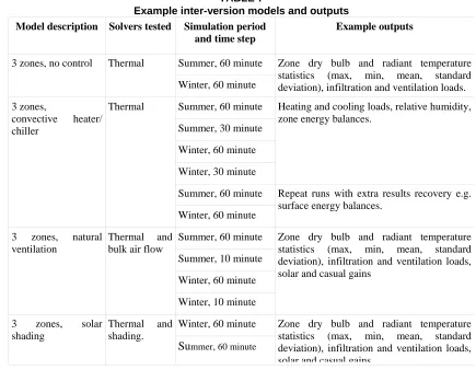
accepted Standards in that area – e.g. expanded ASHRAE 140 tests and new CEN standards. Table 7 shows 17

a subset of these benchmark models currently run after each program update. 18

19

TABLE 7 20

Example inter-version models and outputs 21

Model description Solvers tested Simulation period and time step

Example outputs

3 zones, no control Thermal Summer, 60 minute Zone dry bulb and radiant temperature statistics (max, min, mean, standard deviation), infiltration and ventilation loads. Winter, 60 minute

3 zones,

convective heater/ chiller

Thermal Summer, 60 minute Heating and cooling loads, relative humidity, zone energy balances.

Summer, 30 minute

Winter, 60 minute

Winter, 30 minute

Summer, 60 minute Repeat runs with extra results recovery e.g. surface energy balances.

Winter, 60 minute

3 zones, natural ventilation

Thermal and bulk air flow

Summer, 60 minute Zone dry bulb and radiant temperature statistics (max, min, mean, standard deviation), infiltration and ventilation loads, solar and casual gains

Summer, 10 minute

Winter, 60 minute

Winter, 10 minute

3 zones, solar shading

Thermal and shading.

Winter, 60 minute Zone dry bulb and radiant temperature statistics (max, min, mean, standard deviation), infiltration and ventilation loads, solar and casual gains

Su

22 23

SENSITIVITY STUDY – ANISOTROPIC DIFFUSE SKY MODELS 24

One benefit from including the tests so that they are easily available in the program is that it enables 25

has resulted in significant changes to predictions. In both cases, it is possible to use diagnostic tests to 1

check the impact on specific program areas for which the diagnostic tests are designed or on the impact 2

with respect to Standards compliance. The fact that a large number of tests are involved increases the 3

chances of detecting the impact of a change. 4

To demonstrate the use of the new facility, a study was undertaken of alternative anisotropic diffuse 5

sky models. There have been numerous studies of such models but there is no definitive answer at present 6

as to which is the most appropriate model to use. A good review of the current state of the art is given by 7

Muneer (1997). 8

It was decided to run alternative algorithms for two cases: 9

1. Using low-level diagnostic cases focussing on accentuating the differences in solar algorithms. The 10

low mass in-depth sensitivity test case 250-220 was chosen as it involved altering the external surface 11

absorptance in the test building from 0.1 to 0.9, with no other changes. 12

2. Using Case 960 - a more realistic case with a sunspace – two zones (back zone and sun zone) separated 13

by a common wall. The back zone is of lightweight construction and the sun room of heavyweight 14

construction. 15

Running the tests was straightforward. ESP-r was sequentially configured with the alternative 16

algorithms enabled. The identified test cases were selected and the automated simulation and results 17

recovery initiated. The algorithms invoked in this test were Perez (1990), Perez (1987), Klucher (1979) and 18

an isotropic model. 19

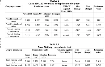
Tables 8 and 9 set out the results directly obtained from the program for the two cases selected. The 20

ranges quoted are given in informative annex to the ASHRAE 140 Standard based on the results from 21

programs in the original BESTEST simulations published in 1995. The column headed “CHECK” shows 22

whether the current results (for the Perez 1990 model) are inside or outside the corresponding range. The 23

values given as “reference values” are those obtained by ESP-r in the original IEA Annex 21 BESTEST 24

study and also published in the ASHRAE Standard 140 annex. All the ranges and reference values are 25

stored in a file, together with the model, so they can be easily updated should new ranges be obtained. Of 26

more practical use, the reference values can be updated with the results obtained in the previous program 27

release, so that it is easy to detect whether predictions have changed. 28

29

TABLE 8 30

Case 250-220 low mass in-depth sensitivity test 31

Output parameter Simulation result CHECK (against Perez 1990)

Min (Range)

Max (Range)

Reference value

Perez 1990 Perez 1987 Klucher 1979

Isotropic

Peak Heating Load

(kW) 0.000 0.000 0.000 0.000 inside -0.007 0.005 -0.001

Peak Cooling Load

(kW) 2.720 2.780 2.560 2.570 inside 1.043 3.699 2.800

Annual Heating

Load (kWh) -2113 -2120 -2085 -2081 inside -2193 -1448 -2193

Annual Cooling

Load (kWh) 3195 3287 3024 3026 outside 1752 3027 3027

32 33

TABLE 9 34

Case 960 high mass basic test 35

Output parameter Simulation result CHECK (against Perez 1990)

Min (Range)

Max (Range)

Reference value Perez

1990

Perez 1987

Klucher 1979

Isotropic

Peak Heating Load

(kW) 2.540 2.530 2.560 2.570 inside 2.410 2.863 2.410

Output parameter Simulation result CHECK (against Perez 1990)

Min (Range)

Max (Range)

Reference value (kW)

Annual Heating Load

(kWh) 2304 2265 2459 2483 outside 2311 3373 2311

Annual Cooling Load

(kWh) 700 741 654 667 inside 411 803 488

Annual Hourly Max

Temperature (˚C) 50.8 51.0 49.4 49.0 inside 48.9 55.3 48.9

Annual Hourly Min

Temperature (˚C) 2.0 2.0 1.6 1.5 inside -2.8 3.9 2.7

Annual Hourly Average Temperature

(˚C)

28.7 29.0 27.9 27.9 inside 26.4 29.0 27.5

1

There are two cases where the predictions fall just outside the indicative ranges when the Perez 1990 2

model is used. These are cases where ESP-r was used to set the suggested limits based on simulations 3

undertaken in the Annex 21 work, and where subsequent changes to the code have pushed predictions 4

outside the limits. Although there are differences in predictions caused by the choice of solar model, they 5

are generally small compared to the range given in ASHRAE Standard 140. In these simulations, the 6

internal convection coefficients were chosen to be the same as in the original Annex 21 study. As will be 7

shown in the following section, this may not be appropriate. 8

9

S

This section examines the sensitivity of the heating loads predicted for BESTEST case 600 upon the 11

modelling of internal surface convection. 12

Modelling Internal Surface Convection 13

The convective heat exchange between internal building surfaces (walls, windows, etc.) and indoor air 14

significantly affects a room's energy balance. For example, this mechanism determines the timing and 15

degree to which solar gains absorbed by internal surfaces warm the room air. The common approach for 16

modelling this heat flow path within dynamic whole-building simulation programs is to employ the so-17

called well-stirred assumption (refer to Figure 3). This treats the room air as uniform and characterizes 18

surface convection heat transfer (

q

′′

19

between the room air and the internal surface. 20

Numerous researchers have examined the sensitivity of simulation predictions to the modelling of 21

internal convection (Waters 1990, Irving 1982, Bauman et al 1983, Alamdari et al 1984, Spitler et al 1991, 22

Clarke 1991, Lomas 1996, Fisher and Pedersen 1997, Beausoleil-Morrison and Strachan 1999 and 23

Beausoleil-Morrison 2001). They have demonstrated that predictions of energy demand and consumption 24

can be strongly influenced by the choice (made by program developer or user) of hc algorithm. Energy

25

prediction sensitivities in the order of 20-40% have been observed. More significantly, in some cases the 26

predicted benefits from design measures were found to be sensitive to the approach used to model internal 27

surface convection. Despite this, most simulation programs still employ simplified approaches. 28

Clearly more detailed calculation approaches are required for this significant heat transfer path. A flow 29

responsive method to improve the modelling of internal surface convection was put forward by Beausoleil-30

Morrison (2002) and implemented into ESP-r. Known as the adaptive convection algorithm (ACA), it 31

employs a series of automated appraisals and user prompts during the problem definition stage to appraise 32

conditions in each room. Each internal surface is attributed with a set of hc equations appropriate for the

33

flow conditions anticipated over the duration of the simulation. As the simulation progresses, a controller 34

monitors critical simulation variables to assess the flow regime. Based upon this assessment, the controller 35

dynamically assigns (for each surface) an appropriate hc algorithm from amongst the set attributed at the

36

problem definition stage. At the basis of this flow responsive method is a scheme for broadly classifying 37

the principle convective regimes encountered within buildings and a suite of 28 hc correlation equations.

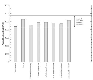
Sensitivity Analysis 1

Eight simulations were performed with the case 600 model to investigate the impact of internal surface 2

convection modelling. ESP-r's default internal convection treatment was employed in the first simulation. 3

With this, the Alamdari and Hammond (1983) hc correlations for buoyancy-driven flow are used for all

4

surfaces and at all time-steps of the simulation (a common approach with simulation programs and the 5

approach usually employed by ESP-r users). This resulted in an annual heating load of 4,387 kWh. 6

The BESTEST procedure allows the use of fixed convection coefficients (internal and external) for 7

programs which do not calculate hc. The results reported for the majority of the reference programs in

8

BESTEST (and thus in the informative annexes of ASHRAE Standard 140) employed this technique. A 9

second simulation was performed with these fixed values. This resulted in an annual heating load of 5,266 10

kWh, 20% greater than the first simulation. These two results are contrasted in Figure 4, which also plots 11

the range of the results produced by the BESTEST reference programs. The sensitivity in the heating load 12

predictions to this one change in the modelling of convection is seen to span fully 62% of the range of 13

differences of all programs considered in BESTEST. 14

The Alamdari and Hammond hc correlations employed in the first simulation are applicable for purely

15

buoyant flow, and only where buoyancy is caused by a temperature difference between a surface and the 16

surrounding room air. They are not appropriate for cases where buoyancy is generated by a heating device, 17

such as a radiator, or when the convective regime is generated by a forced-air device. The BESTEST 18

specification indicates that heating and cooling is supplied by a convective system. Consequently, it is 19

believed that the use of the Alamdari and Hammond correlations is not appropriate in this case and 20

therefore alternate hc modelling methods are investigated here.

21

Khalifa (1989) conducted experiments in a room-sized test cell to produce correlations specific to 22

internal convection within buildings. The test cell's configuration was varied and experiments repeated to 23

assess a number of common convection regimes. Convective heat transfer at internal surfaces was not 24

measured directly, but rather hc was derived from temperature and heat input measurements. It is important

25

to note that radiant exchange was neglected in this derivation. As such, it is believed that Khalifa's results 26

tend to overestimate hc. Although there are insufficient data available to determine the degree of

27

overestimation, the errors would be greatest in the cases with large temperature differences between 28

surfaces (such as a hot radiator facing a cold window). Notwithstanding, Khalifa's work represents a 29

significant contribution, as he provides hc data for room configurations not analyzed by others.

30

Khalifa's correlations for rooms heated with circulating fan heaters were employed in the third and 31

fourth simulations. In the fourth simulation Khalifa's hc correlation for vertical surfaces which experience

32

impinging flow from the convective heater were employed for all walls and the windows, whereas in the 33

third simulation Khalifa's hc correlation for walls that do not experience impinging flow were employed.

34

These two simulations resulted in annual heating loads that lie in between those of the first two simulations, 35

being 4.4% and 11.3% greater than the first simulation. 36

These first four simulations employ non-adaptive convection calculations, in that the methods used to 37

calculate hc do not vary on a time-step basis. The adaptive convection algorithm, described earlier, was

38

invoked for the next three simulations reported in Figure 4. All internal surfaces were attributed with 39

convection calculation control data for the case of rooms heated with convective heaters that circulate air 40

within the room. With this approach the simulator toggles between hc calculation methods as the simulation

41

progresses. When the simulator senses that the heater is operating it employs the appropriate Khalifa 42

correlations. And when it senses that the heater is inoperative it switches to the Alamdari and Hammond 43

correlations, assuming that the flow is then governed by buoyant forces generated by surface-air 44

temperature differences. Three variants were assessed. In the fifth simulation, all vertical surfaces were 45

attributed with the Khalifa correlation for impinging flow. In the sixth simulation it was assumed that only 46

the south facing wall and the windows experienced impinging flow. And in the seventh simulation the east, 47

north, and west walls received the impinging flow. As illustrated in Figure 4 there is a 3.5% range in the 48

annual heating loads predictions between these three ACA simulations and a significant difference between 49

these three and the first simulation. 50

Finally, the eighth simulation was performed with the ACA but in this case the surfaces were attributed 51

with convection correlations appropriate for mixed buoyant and forced flow in which the HVAC system 52

circulates heated or cooled air to the room. This resulted in an annual heating load prediction that was 17% 53

greater than the first simulation. 54

Based upon the information provided in the BESTEST procedure it is impossible to conclude which of 55

simply does not provide sufficient information to specify the convective regimes. As these results show, 1

details such as which surfaces receive impinging flow from a convective heater or how cooling is achieved 2

can have an influence that is significant in the context of a validation exercise. Given this, future validation 3

efforts should either specify convective regimes in a level of detail that is commensurate with the 4

modelling of other significant heat transfer processes, such as envelope transmission and solar gains, or 5

convection coefficients should be fixed to prevent erroneous noise between reference program results. 6

7

CONCLUSIONS 8

Validation models and tests can be time consuming to set up and as a consequence, programs are only 9

irregularly checked. There is a clear need for regular checking of program outputs against a whole range of 10

standard tests, and also for regular assessment of what are deemed to be acceptable ranges for predictions. 11

This requirement will become more pressing as simulation-based standards are introduced. The work 12

discussed in this paper shows how it is possible to embed these tests to make it easy for developers and user 13

to apply them. The benefits are: 14

• Program developers can check the impact of code modifications, algorithmic substitution etc. 15

• Developers can check compliance with regulations. 16

• User confidence is improved. 17

• Users can confirm that their installation is correct and check Standards compliance themselves. 18

• It avoids the repetition of constructing the models set out in the validation tests and therefore it 19

reduces the associated possibility of error. It is sometimes difficult to construct the models when 20

unusual modelling assumptions are required. 21

• Frequent checking will confirm the fact that a program continues to be within the specified 22

tolerance bands. This is important as most state-of-the-art programs are under constant 23

development. 24

The question of what are acceptable ranges for predictions in comparative validation tests is difficult to 25

answer. If the programs are allowed to model the various heat transfer processes with their own methods, 26

then the indicative tolerance bands will be wide (as in the case of the ASHRAE Standard 140 fabric and 27

envelope tests) and programs with errors could still fall within the specified bands. On the other hand, if the 28

way in which the processes are modelled is prescribed in detail, then tolerance bands will be narrow. 29

However, in this case, more detailed and accurate ways of modelling may give out-of-range predictions. A 30

related question is, if a program is used with a simplified way of modelling the particular heat transfer 31

process in order to fall within the tolerance bands, whether this means the program always has to be used in 32

this mode in order to claim compliance with Standards. 33

It is believed the way forward is to develop guidance on the most appropriate way to model the 34

important heat transfer processes. As shown in this paper, it is particularly important for the internal 35

convective transfer process - validation tests should indicate the flow regime so appropriate algorithms can 36

be selected, and research undertaken to identify appropriate correlations for situations where they are not 37

currently available. In this way, it should be possible to reduce the acceptable bands for program 38

predictions without being unnecessarily prescriptive. This will also reduce the likelihood of a simulation 39

program being selected for design work based on the fact it typically predicts, say, lower cooling loads. 40

It is intended that other tests, in addition to those described in this paper, will be put within the same 41

structure described in this paper. This will include further tests within ASHRAE and CEN Standards, 42

together with other tests being developed within IEA projects. 43

44

REFERENCES 45

Alamdari F. and Hammond G.P. (1983), ‘Improved Data Correlations for Buoyancy-Driven Convection in 46

Rooms’, Building Services Engineering Research and Technology, 4 (3) 106-112. 47

Alamdari F., Hammond G.P., and Melo C. (1984), ‘Appropriate Calculation Methods for Convective Heat 48

Transfer from Building Surfaces’, Proc. 1st U.K. National Conf. on Heat Transfer, (2) 1201-1211. 49

ANSI/ASHRAE, Standard 140-2004 (2004), Standard Method of Test for the Evaluation of Building 50

Energy Analysis Computer Programs, ASHRAE, Atlanta, Georgia. 51

Bauman F., Gadgil A., Kammerud R., Altmayer E., and Nansteel M. (1983), ‘Convective Heat Transfer in 52

Beausoleil-Morrison I. and Strachan P. (1999), ‘On the Significance of Modelling Internal Surface 1

Convection in Dynamic Whole-Building Simulation Programs’, ASHRAE Transactions 105 (2) 929-2

940. 3

Beausoleil-Morrison I. (2001), ‘An Algorithm for Calculating Convection Coefficients for Internal 4

Building Surfaces for the Case of Mixed Flow in Rooms’, Energy and Buildings 33 (4) 351-361. 5

Beausoleil-Morrison I. (2002), ‘The Adaptive Simulation of Convective Heat Transfer at Internal Building 6

Surfaces’, Building and Environment, 37 791-806. 7

Ben-Nakhi A. and Aasem E.O. (2002), ‘Development and Integration of a User-Friendly Validation 8

Module within Whole Building Dynamic Simulation’, Energy Conversion and Management, 44 (1), 9

pp53 – 64. 10

Bloomfield D. P. (1999), ‘An Overview of Validation Methods for Energy and Environmental Software’, 11

ASHRAE Transactions, Vol 5, Part 2, SE-99-6-1. 12

CEN (2004), prEN ISO 13791: Thermal Performance of Buildings – Calculation of Internal Temperatures 13

of a Room in Summer without Mechanical Cooling – General Criteria and Validation Procedures, 14

ISO/FDIS 13791:2004. 15

Clarke J.A. (1991), Internal Convective Heat Transfer Coefficients: A Sensitivity Study, Report to ETSU, 16

University of Strathclyde, Glasgow U.K. 17

ESRU (2005), The ESP-r System for Building Energy Simulations, University of Strathclyde, Glasgow, 18

UK. (http://www.esru.strath.ac.uk). 19

Fisher D.E. and Pedersen C.O. (1997), ‘Convective Heat Transfer in Building Energy and Thermal Load 20

Calculations’, ASHRAE Transactions, 103 (2) 137-148. 21

Irving S.J. (1982), ‘Energy Program Validation: Conclusions of IEA Annex 1’, Computer Aided Design, 14 22

(1) 33-38. 23

Jensen S.O. (ed) (1993), Validation of Building Energy Simulation Programs, Part I and II, Research 24

Report PASSYS Subgroup Model Validation and Development, CEC, Brussels, EUR 15115 EN. 25

Judkoff R., Wortman D., O’Doherty R. and Burch J. (1983) ‘A Methodology for Validating Building 26

Energy Analysis Simulations’, SERI/TR-254-1508, Golden, Colorado, USA: Solar Energy Research 27

Institute, now National Renewable Energy Laboratory. 28

Judkoff R. and Neymark J. (1995), IEA Building Energy Simulation Test (BESTEST) and Diagnostic 29

Method, IEA Annex 21/Task 12 Co-operative Project, Final Report. 30

Khalifa A.J.N. (1989), Heat Transfer Processes in Buildings, PhD Thesis, University of Wales College of 31

Cardiff, Cardiff UK. 32

Klucher T.M, (1979), ‘Evaluation of models to predict insolation on tilted surfaces’, Solar Energy 4,14. 33

Lomas K.J. (1996), ‘The U.K. Applicability Study: An Evaluation of Thermal Simulation Programs for 34

Passive Solar House Design’, Building and Environment, 31 (3) 197-206. 35

Lomas K.J., Eppel H., Martin C. and Bloomfield D. (1994), Empirical Validation of Thermal Building 36

Simulation Programs using Test Room Data, IEA Annex 21/Task 12 Co-operative Project, Final 37

Report, Vols 1,2 and 3. 38

Muneer T., (1997), Solar radiation and daylight models for the energy efficient design of buildings, 39

Architectural Press, Oxford. 40

Perez R., Seals R., Ineichen P., Stewart R. and Menicucci D. (1987), ‘A new simplified version of the Perez 41

diffuse irradiance model for tilted surfaces’. Solar Energy, Vol.39 No.3, 221-232. 42

Perez R., Ineichen P., Seals R., Michalsky J., and Stewart R. (1990), ‘Modeling daylight availability and 43

irradiance components from direct and global irradiance’, Solar EnergyVol.44 No.5, pp271-289. 44

Spitler J.D., Pedersen C.O., and Fisher D.E. (1991), ‘Interior Convective Heat Transfer in Buildings with 45

Large Ventilative Flow Rates’, ASHRAE Transactions, 97 505-515. 46

Strachan P.A., Kokogiannakis G. and Macdonald I.A. (2005), ‘Encapsulation of Validation Tests in the 47

ESP-r Simulation Program’, Building Simulation ’05, Montreal, Canada. 48

Waters J.R. (1980), ‘The Experimental Verification of a Computerised Thermal Model for Buildings’, 49

Building Services Engineering Research & Technology, (1) 76-82. 50

1 2 3 4 5 6 7 8 9 10 11 12 13 14 15 16 17 18 19 20 21 22 23 24 25 26 27 28 29 30 31 32 33 34 35 36 37 38 39 40 41 42 43 44 45 46 47

Figure 1: Implementation details 48

49 50 51 52

Standards

ASHRAE 140-2004

(building envelope tests) CEN

Cooling loads

Group 1 ...Group 4 (e.g. HM basic sensitivity tests)

Free Float tests (e.g.

600FF) Individual tests (e.g. 195)

All tests (groups and individuals)

Pair of models selected to be processed (e.g. 200-195 *,

210-200 *)

Free Float tests selected to be processed (e.g. 600FF *, 650FF *)

Individual tests selected to be processed

(e.g. 200 *, 650FF *)

Simulation invokes automatically and sequentially for model(s) selected (e.g. For 200-195: simulates model 195 and then model 200).

Recovery of the simulation results invokes automatically and sequentially for each model based on output data specified in the data recovery files. A results file is created

for each model selected.

Output data is processed (e.g. differences are calculated for the in-depth cases) and results compared to tabulated limits.

Predicted values, maximum and minimum ASHRAE published limits, a inside/outside range check, and results from a previous standard distribution of ESP-r are displayed

or sent to an external file. ASHRAE 140-2004

(HVAC tests) CEN 13791

1

2

1

Figure 3: Well-stirred convection model 2

1

2

Figure 4: Sensitivity of case 600's annual heating load to internal convection modelling 3