Analysis of yeast codon usage patterns using the movable ORF collection

(1)

Rochester Institute of Technology

RIT Scholar Works

Theses Thesis/Dissertation Collections

5-1-2007

Analysis of yeast codon usage patterns using the

movable ORF collection

Nunut Butarbutar

Follow this and additional works at:http://scholarworks.rit.edu/theses

This Thesis is brought to you for free and open access by the Thesis/Dissertation Collections at RIT Scholar Works. It has been accepted for inclusion in Theses by an authorized administrator of RIT Scholar Works. For more information, please [email protected].

Recommended Citation

(2)

ANALYSIS OF YEAST CODON USAGE PATTERNS USING

THE MOVABLE ORF COLLECTION

Approved: _____________________________________________ Thesis Advisor

_____________________________________________ Director of Bioinformatics

Submitted in partial fulfillment of the requirements for the Master of Science Degree in Bioinformatics at the Rochester Institute of Technology

(3)

Thesis Committee

Thesis Advisor

Dr. Shuba Gopal

School of Life Science

Department of Bioinformatics Rochester Institute of Technology

Committee Member

Dr. Gary Skuse

School of Life Science

Department of Bioinformatics Rochester Institute of Technology

Dr. James Halavin

(4)

Thesis/Dissertation Author Permission

Title of thesis or dissertation: Analysis of yeast codon usage patterns using the movable ORF collection.

Name of author: Nunut B Butarbutar Degree: Master of Science

Program: Bioinformatics College: Science

I understand that I must submit a print copy of my thesis or dissertation to the RIT Archives, per current RIT guidelines for the completion of my degree. I hereby grant to the Rochester Institute of Technology and its agents the non–exclusive license to archive and make accessible my thesis or dissertation in whole or in part in all forms of media in perpetuity. I retain all other ownership rights to the copyright of the thesis or dissertation. I also retain the right to use in future works (such as articles or books) all or part of this thesis or dissertation.

Print Reproduction Permission Granted:

I, Nunut Butarbutar, hereby grant permission to the Rochester Institute Technology to reproduce my print thesis or dissertation in whole or in part. Any reproduction will not be for commercial use or profit.

Signature of Author: __________________________________ Date: ____________

Inclusion in the RIT Digital Media Library Electronic Thesis & Dissertation (ETD) Archive

I, Nunut Butarbutar, additionally grant to the Rochester Institute of Technology Digital Media Library (RIT DML) the non–exclusive license to archive and provide electronic access to my thesis or dissertation in whole or in part in all forms of media in perpetuity. I understand that my work, in addition to its bibliographic record and abstract, will be available to the world–wide community of scholars and researchers through the RIT DML. I retain all other ownership rights to the copyright of the thesis or dissertation. I also retain the right to use in future works (such as articles or books) all or part of this thesis or dissertation. I am aware that the Rochester Institute of Technology does not require registration of copyright for ETDs. I hereby certify that, if appropriate, I have obtained and attached written permission statements from the owners of each third party copyrighted matter to be included in my thesis or dissertation. I certify that the version I submitted is the same as that approved by my committee.

(5)

ABSTRACT

The relationships between codon usage and protein expression levels have been extensively studied in various organisms. Highly expressed genes have often been shown to have stronger compositional codon bias. However, previous studies often failed to separate the effects of regulatory control from codon usage patterns. These studies have also been deficient with respect to both gene and protein coverage.

In this study, we investigated the role of codon usage patterns in Saccharomyces cerevisiae using the Movable Open Reading Frame (MORF) collection library. The new collection is based on the recent annotation of yeast genome and is made with high– efficiency and high–fidelity cloning procedures, providing the most complete collection of ORFs available for any organism. It is also the first collection of proteins where all the proteins are under common regulatory control. Thus, it provides the best opportunity to investigate the specific role of codon usage in determining levels of protein expression.

(6)

LIST OF FIGURES

Figure 1 – Graphical representation of codon usage space...3

Figure 2 – Diagram of MORF expression vector ...6

Figure 3 – MORF expression...11

Figure 4 – Research methodology ...15

Figure 5 – Diagram of sliding window ...26

Figure 6 – Rare codon counts per quartile ...31

Figure 7 – Positions specific rare codon distribution in the first 100 codon ...33

Figure 8 – Position specific rare codon in the first 100 codon shown with errors bars. ...34

(7)

LIST OF TABLES

Table 1 – Measuring dependencies between position 4 (N4) and 5 (N5)...17

Table 2 – Codon usage profile of MORF. ...20

Table 3 – Protein classification using the entire sequence length with codon adaptation index scores as the basis for classification. ...22

Table 4 – Codon log value ...23

Table 5 – Classification based on protein expression levels using the log likelihood method. ...24

Table 6 – Protein classification using the early codons ...25

Table 7 – Performance of Log likelihood method using rare codon clusters ...26

Table 8 – Performance of Log likelihood method using a threshold cut off value ...27

Table 9 – Rare codons with a frequency of less then 13 per 1000 codons ...29

Table 10 – Rare codon defined by the new definition ...30

Table 11 – Performance of log likelihood method scoring only the 17 codon positions. ...35

Table 12 – A portion of the 300 x 300 chi–squared matrix. ...36

Table 13 – Significant dependence in nucleotide positions...37

Table 14 – Performance of log likelihood method scoring dependent position ...38

(8)

Introduction

The cell is of one the most ingenious designs found in nature. It contains a factory specializing in the production of proteins encoded by a gene. Interestingly enough, the cell itself is managed by its own product, the proteins. These proteins provide signals and instructions which tell the cell what to do and when to do it. They are a vital part of the biological system, taking on numerous roles such as catalyzing biochemical reactions and maintaining structural integrity. An imbalance in protein levels, caused by the over– or under–expression of a protein, can often lead to chronic diseases. Thus, various mechanisms have been developed to ensure that protein concentrations are always balanced. This regulatory control comes in many different forms, for example feedback inhibition or competitive inhibitors. As a consequence, proteins are often expressed in low abundance.

In order to understand the biological function of proteins, current laboratory techniques require large quantities of protein samples. Since proteins are typically expressed in low abundance in their natural source, scientists have developed eukaryotic vectors for synthesizing functional proteins outside the native host. Studies have successfully utilized eukaryotic expression vectors to synthesize functional proteins from a variety of hosts [1]. In theory the process is relatively simple. After the protein of interest has been inserted into an expression vector, the cell is allowed to grow while synthesizing this new protein. This process, known as expression in heterologous hosts, generally yields sufficient quantities of most soluble proteins.

(10)

can be toxic to the host itself. In other cases, the proteins may not be expressed or are expressed in very low quantities. The success expression of recombinant proteins often depends on the quality of the DNA sequence. Adjusting the sequence composition can yield dramatic increases in protein sequence because of the degenerate codon issue. The genetic code consists of 64 codons which code for 20 amino acids. Since several codons code for the same amino acid, a string of 99 amino acids sequence can be represented by billions of codon combinations. The DNA sequence used to encode a protein in one organism is often quite different from the DNA sequence used to encode the same protein in another organism [2].

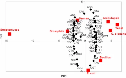
To further complicate the picture, a wealth of research has now shown differential synonymous codon usage between different organisms. This flexibility at the DNA level is not used randomly. Instead, organisms tend to use a subset of all possible codons. As a result, expression of these proteins in a different organism is likely to suffer [3]. Codon usage has been studied in a number of different organisms. Figure 1 displays the average codon preference of genomes from eight commonly studied organisms [2]. It has been seen that Streptomyces coelicolor has the most extreme codon usage profile [2]. In this organism almost every “wobble” position (the third base in each codon, where much of the degeneracy of the genetic code resides) is a G or C, resulting in a high GC context [2]. Figure 1 also shows that Saccharomyces cerevisiae, Caenorhabditiis elegans and

(11)

[image:11.612.108.514.141.393.2]

genome of a different species. You must also consider whether the new host species’ codon usage characteristics are similar to those of your native host.

Figure 1 – Graphical representation of “codon usage space”. Principle Component Analysis comparing

the average codon preference in eight organisms [2].

Codon Usage and Predicting Protein Expression Levels

(12)

when proteins from two thermoacidophilic organisms (Sulfolobus solfataricus and

Thermoplasma acidophilum) were being expressed in E. coli, researchers found that the recombinant proteins from T. acidophilum were expressed at higher levels than S. solfataricus. Codon usage analysis in both thermoacidophilic organisms revealed a high proportion of rare codons which are rarely used in E. coli. However, the S solfataricus

sequence was found to have clusters of rare codons at the beginning of the transcript. Thus, the difference in expression levels was thought to be influenced by the presence of these rare codon clusters [12].

One common strategy to improve expression is to alter the frequency of rare codons in the target genes so they closely reflect the codon usage of the host, without modifying the amino acid sequence of the encoded protein [2]. For example in E.coli, genes containing high levels of infrequently used codons such as AGG and AGA (both arginine) was found to be expressed at a lower level compared to those with few AGG and AGA codons [11]. Therefore, replacing rare codons with preferred codons would theoretically increase the level of expression. This process of codon optimization has been successfully applied in Mus musculus where an increase of over 50–fold was observed. Other studies in Triticum estivum generated a 4 to 17 fold increase [13] and various experiments in E.coli have generated similar results [14, 15].

(13)

There are many factors that affect gene expression such as regulatory processes that alter the expression of the gene [17]. Specific promoters and regulators located upstream and downstream of the initiation codon are also known to act as translational enhancers. These sequences are known to exert control on the overall level of gene expression and hence can affect protein expression levels [18].

Previous analysis of codon usage and protein expression have also been deficient with respect to both gene and protein coverage. The introduction of mutations during cloning, incomplete/incorrect annotation of genes in the collections and fusion of affinity tags to the N termini of cloned genes (which is likely to interfere with targeting of proteins destined for the secretory pathway), and the presence of complex regulatory mechanisms for the control of gene expression have all limited our ability to assess the impact of codon usage on protein expression levels in heterologous hosts [19].

A New Way to Analyze Codon Usage and Protein Expression Levels

(14)

The MORF library is one of the most comprehensive collections of S. cerevisiae

[image:14.612.226.422.233.368.2]

ORF containing 93.2% of verified yeast ORF’s in SGD with over half of the collection completely sequenced [19]. The broad range of coverage provides the ideal data set for evaluating codon usage and its impact on protein expression within yeast.

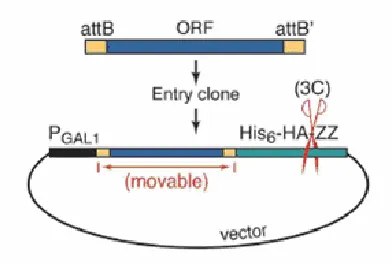
Figure 2 – Diagram of MORF expression vector.The ORF (blue) sequences are flanked by directional

attB sequence (yellow). All the sequences are expressed under the PGAL promoter and terminally tagged by

4.8 kDA tag (green) [19].

The structural design of the MORF plasmid can be seen in figure 2. All the ORFs are expressed under a PGAL promoter, starting at the natural N–terminal methionine and ending with a fusion of the C–terminal amino acid tag (His6– HAepitope–3C protease site

(15)

expression levels.26% of the MORF collections are highly expressed, 37% are expressed at a medium level, 30% are lowly expressed and 7% are undetectable [19]. Due to the nature of the plasmid, these differences in expression levels can be attributed to the intrinsic properties of the yeast DNA sequence.

By utilizing the MORF collections, this work hopes to overcome the most significant limitations of previous libraries. Expression information derived from this library is cleaner compared to previous experimentally generated data. The common regulatory control of each MORF also eliminates the limitation in previous studies. Therefore, it is reasonable to expect that the MORF data set can provide an appropriate venue to investigate the correlation between expression levels and its sequence composition.

Codon Usage in S. cerevisiae

Since the MORF collection is based in S. cerevisiae, it is important to understand the factors that affect protein expression levels in this organism. The codon usage profile of S. cerevisiae has marked a preference for 25 of the 61 possible coding triplets [7]. Genes containing high levels of preferred codons stand a higher chance of being expressed than those with unfavorable codons. In order to quantify these preferences, a wide variety of techniques have been developed. These include codon preference bias [21], frequency of optimal codons [22], codon bias index [4] and codon preference statistic [23].

(16)

sequence composition [9]. It uses the occurrence of specific codons in a gene sequence to predict whether a gene is likely to be highly expressed [9]. However, a recent study has shown that the metric is highly biased and limited in predicting protein expression levels [5]. Since the method relies on codon profiles obtained from 24 highly expressed genes, the method carries a strong bias towards detecting highly expressed genes [5]. Additionally, the CAI only measures the degree of preference not the nature of that preference, thus it cannot be used to assess the likely compatibility between a gene and its candidate host [5]. The gene might have a strong bias that results in high codon CAI but these preferences could be quite different for another gene [2].

Earlier work has suggested that the codon composition in the early portion of the transcript can dramatically affect protein expression levels [12, 24]. Analyzing the composition of codons in the beginning of the transcript could shed some light on the relationship between codon usage and its expression levels. There is some evidence of nucleotides, located near the start codon, exerting an unusual amount of influence on the level of protein expression [18, 30]. These dependencies can be modeled through the Maximal Dependence Decomposition (MDD) method. MDD was developed to capture significant dependencies between nucleotide positions. It was originally proposed as a method to detect splice sites between introns and exons. We utilized this approach to see if certain nucleotide level dependencies might correlate with protein expression levels. The positional preference effect could be used as another indicator of expression.

(17)

(18)

MATERIALS AND METHOD

Movable Open Reading Frame (MORF)

The MORF collection contains sequence analyzed S. cerevisiae open reading frames (ORFs) that were designed to maximize gene and protein representation in a high–quality expression library [19]. While the MORFs are constructed in a similar fashion, the presence, amount, size and quality of 5573 ORF fusion proteins that were examined showed substantial differences in protein expression levels. Based on the expression levels, these MORFs can be classified into three categories: 1427 of highly expressed MORFs (~ 1+ mg/L), 2116 medium MORFs (~0.1 mg/L), 1645 lowly expressed MORFs (~0.01 mg/L), with 385 MORFs being undefined [19]. In order to ensure the accuracy and consistency of these classifications, the results were checked for consistency against two sources of data. These were:

1. The University of San Francisco (UCSF) Native Expression Database provides information on the number of protein molecules observed in cells [25]. We used these data to define high expressing MORFs as those that had high expression in the MORF data set and at least 5000 molecules per cell as observed by the UCSF group. For low MORFs, we selected those that were low expressors in the MORF data and had fewer than 5000 molecules per cell based on the UCSF data set.

(19)

[image:19.612.111.535.74.208.2]

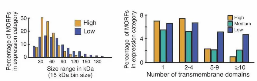
Figure 3 – MORF expression. (A) Molecular weight distribution of MORF proteins, with out the terminal

tag, in high (yellow) and low (blue) expression categories (B) Effect of transmembrane domain on

expression levels. MORF’s in each expression category were sorted into the bins indicated (yellow) High

expression (green) medium expression (blue) low expression [19].

(20)

Calculating Codon Frequency

A majority of prokaryotic and eukaryotic organisms are known to display non– random codon usage. In fact, the differential preference over a codon has been previously used to identify highly expressed genes [27-29]. To assess codon usage, we first need to calculate the frequency with which any given codon is observed in a set of sequences. For

each codon

χ

_i coding for amino acid AAi, we calculated the absolute codon frequency for the set of high MORFs and similarly for the low MORFs. We calculated codon frequency by taking the occurrences of codon N

( )

χ_i over the total number of codons of all the sequences in each set (high and low). We then multiply this value by 1000 to get the frequency of a given codon per 1000 codons. This metric provides a normalized codon frequency for the high and low expressing MORFs.

( )

61

1

(

_i

)

i

1000

i

N

f

N

χ

=

×

∑

...(1)

Codon Adaptation Index (CAI) Model

(21)

L

w

=

CAI

L = k k

1

⎟⎟

⎠

⎞

⎜⎜

⎝

⎛

∏

...(2)

Here, wk is the relative adaptiveness of the kth codon in a gene with L codons. The relative adaptiveness of each codon is defined as the ratio between the frequencies of the codon over the frequency of the major synonymous codon for the same amino acid. Usually, this set is made up of highly expressed genes and thus, the CAI can be use to predict highly expressed genes [9]. The CAI score ranges from 0 to 1, where a higher score suggests that a given gene is likely to be expressed at high levels.

Log–Likelihood Model

The Log likelihood method attempts to model protein expression levels based on observed codon usage difference between the two expressing groups. Compared to the CAI, this method is based on a somewhat broader set of not only highly expressed but also lowly expressed Genes. The first step in log likelihood model is to obtain a profile which highlights the difference between high and low MORFs. For each codon

χ

icoding

for an amino acid, we calculated codon log likelihood ratio C(χi) by taking the log (base 10) ratio of the frequency of the codon as expressed in high MORFs fhigh(

χ

i) over the frequency of the same codon in low MORFs

f

_low

(

χ

_i

)

. The ratio is therefore:

)

(

)

(

log

)

(

₁₀ i low i high i

f

C

χ

(22)

A log likelihood score is then obtained by summing the codon log ratios across all the codons in a MORF sequence. In a given sequence, we summed the log likelihood ratios

) ( _i

C χ for each codon observed to obtain a log likelihood score for the overall sequence:

∑

=

l

1 i

)

(

Score

Likelihood

Log

C

χ

_i _...(4)

Here, )C(χi is the codon log likelihood ratio of the ith codon in a MORF sequence with l

codons. Generally, a more positive score suggests high expression, while a more negative score indicates low protein expression. The actual threshold value for classification of testing sequences, however, varies slightly depending on the training dataset used.

(23)

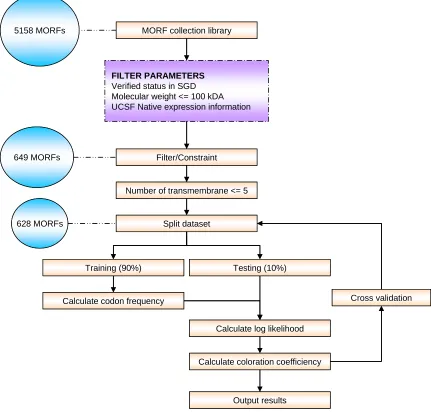
5158 MORFs MORF collection library

FILTER PARAMETERS

Verified status in SGD Molecular weight <= 100 kDA UCSF Native expression information

649 MORFs

628 MORFs

Filter/Constraint

Number of transmembrane <= 5

Split dataset

Training (90%) Testing (10%)

Calculate codon frequency

Calculate log likelihood

Calculate coloration coefficiency

Output results

Cross validation 5158 MORFs MORF collection library

FILTER PARAMETERS

Verified status in SGD Molecular weight <= 100 kDA UCSF Native expression information

649 MORFs

628 MORFs

Filter/Constraint

Number of transmembrane <= 5

Split dataset

Training (90%) Testing (10%)

Calculate codon frequency

Calculate log likelihood

Calculate coloration coefficiency

Output results

[image:23.612.108.539.78.493.2]

Cross validation

Figure 4 – Research methodology. In order to obtain a clean data, the MORF were preprocessed based on

its molecular weight, number of transmembrane and its expression status. MORF that pass these parameters

(24)

For each cross validation run we classified the test sequence into a predicted expression group and determined the frequency of true positive (TP), false positive (FP), true negative (TN) and false negative (FN). The sensitivity, the fraction of those MORFs correctly classified as highly expressed was calculated by the formula:

TP

Sensitivity

TP

FN

=

+

...(5)

Specificity, the fraction of those MORFs correctly classified as lowly expressed, was calculated by the formula:

TN

Specificity

TN

FP

=

+

...(6)

And finally the accuracy, a measure of the overall performance of the classifier, was calculated by the formula:

FN

TN

FP

TP

TN

TP

Accuracy

+

(25)

Maximal Dependence Decomposition (MDD)

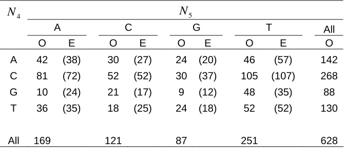
The early portions of the transcript have been suggested to play an important role in determining expression. As such, there may be dependencies among nucleotides early in the transcript. These dependences can be modeled through the maximal dependence decomposition (MDD) method as outlined by Burge and Karlin [30]. MDD is widely used in predicting intron–exon splice signals boundaries. The sequences leading up to the splice signals are often dependent on the certain nucleotide creating a unique dependency profile. By looking at the transitional probability of one nucleotide to another, we can identify specific dependency in the sequence. The first step in MDD is to obtain an observed count from one nucleotide position to every other position in the sequence.

4

N N5

A C G T All O E O E O E O E O A 42 (38) 30 (27) 24 (20) 46 (57) 142 C 81 (72) 52 (52) 30 (37) 105 (107) 268 G 10 (24) 21 (17) 9 (12) 48 (35) 88

T 36 (35) 18 (25) 24 (18) 52 (52) 130

[image:25.612.157.493.366.510.2]

All 169 121 87 251 628

Table 1– Measuring dependencies between nucleotide position 4 (N4) and 5 (N5). The observed

frequency (O) was obtained directly from the combined set of high and low expressor MORFs, while the

theoretical expected frequency (E) was determined from formula 8. The chi–squared calculated by formula

(26)

For example Table 1 displays a 4 x 4 contingency table of observed nucleotide frequency from position 4 to positions 5. Here we can see that nucleotide G (position 4) and nucleotide A (position 5) occurs at a frequency of 10 while the expected theoretical frequency was 24. The expected theoretical count was obtained by taking the ratio of the row sum + column sum over the total observed frequency as outlined below:

(

Row sum Col Sum

)

(

)

Expected

Total Observed

×

= ...(8)

Once the 4 x 4 table is constructed, a chi-squared value was then calculated by taking the difference between observed and expected frequency of each of nucleotide. This value is then squared, divided by the expected frequency and summed across all the nucleotides as shown in the formula below:

(

)

2

ij ij 2

ij

-i j

O E

E

χ

=

∑∑

...(9)

(27)

1) -column (Total

) 1 -row Total ( (df) freedom of

Degrees = × ... (10)

(28)

RESULTS

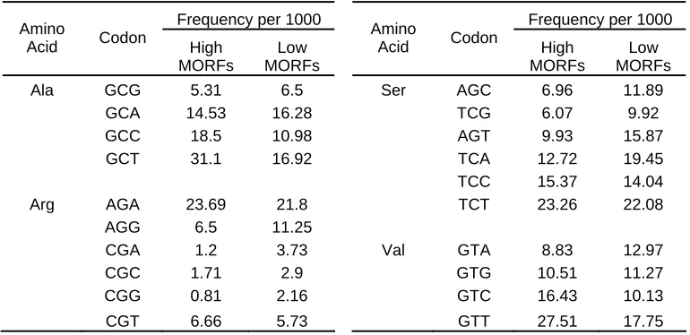
The 5854 MORFs library consist of sequences that were specifically designed to negate the effects of promoters and regulators in protein expression. Despite these efforts, substantial variations in protein expression levels were still detected. Further analysis revealed differential codon usage profile between the highly and lowly expressed MORFs. Therefore, the non–random distribution of synonymous codons within the MORFs sequences appears to be directly influencing protein expression. In our study, we considered two types of MORFs based on their expression levels. We selected 317 highly expressed MORFs and 311 lowly expressed MORFs for analysis. We combined these MORFs for the MDD analysis. For each group, we calculated the absolute codon frequencies as described in Methods. A portion of the results can be seen in Table 2, and the complete table is provided in the Appendices A, B, C.

Frequency per 1000 Frequency per 1000 Amino

Acid Codon High MORFs

Low MORFs

Amino

Low MORFs Ala GCG 5.31 6.5 Ser AGC 6.96 11.89

GCA 14.53 16.28 TCG 6.07 9.92 GCC 18.5 10.98 AGT 9.93 15.87 GCT 31.1 16.92 TCA 12.72 19.45 TCC 15.37 14.04 Arg AGA 23.69 21.8 TCT 23.26 22.08

AGG 6.5 11.25

CGA 1.2 3.73 Val GTA 8.83 12.97

CGC 1.71 2.9 GTG 10.51 11.27

[image:28.612.132.517.425.612.2]

CGG 0.81 2.16 GTC 16.43 10.13 CGT 6.66 5.73 GTT 27.51 17.75

Table 2 – Codon usage profile of High and Low MORFs. The codon usage profile of 317 highly

expressed and 311 lowly expressed MORFs is shown here. Note the differences in codon frequencies for

(29)

As the table suggests, specific differences in codon frequency between the two classes of MORFs can be detected. Highly expressed MORFs often appear to favor one of the synonymous codons while such preferences appear weaker in the low MORFs. For example alanine is encoded by 4 codons, GCG, GCA, GCC, and GCT. If the distribution were truly random, we would expect similar frequency of each of the synonymous codons. Instead, a clear preference for one of the synonymous codons can be seen. In the highly expressed dataset, the alanine GCT codon has a frequency of 31.1 while its synonymous codon GCG only has a frequency of 5.31, a difference of almost 6 fold. Similarly, in the lowly expressed dataset, the codons GCA and GCT appear to be preferred over the GCG codon. Note, however, that there is only a 2 fold difference compared with the 6 fold difference in the high MORFs.

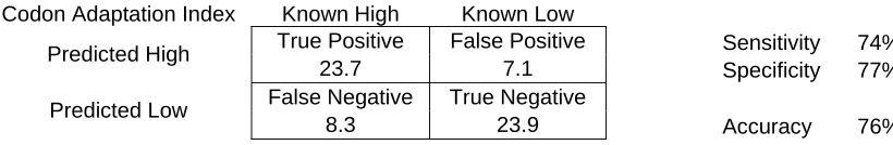
Codon Adaptation Index

(30)

Codon Adaptation Index Known High Known Low

True Positive False Positive Sensitivity 74% Predicted High

23.7 7.1 Specificity 77% False Negative True Negative

Predicted Low

[image:30.612.114.524.87.154.2]

8.3 23.9 Accuracy 76%

Table 3 – Protein classification using the entire sequence length with codon adaptation index scores

as the basis for classification.

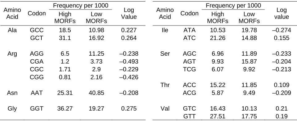
Log likelihood Model

(31)

Acid Codon High MORFs Low MORFs Log Value Amino

Low MORFs

Log value Ala GCC 18.5 10.98 0.227 Ile ATA 10.53 19.78 –0.274

GCT 31.1 16.92 0.264 ATC 21.26 14.88 0.155 Arg AGG 6.5 11.25 –0.238 Ser AGC 6.96 11.89 –0.233 CGA 1.2 3.73 –0.493 AGT 9.93 15.87 –0.204 CGC 1.71 2.9 –0.229 TCG 6.07 9.92 –0.213 CGG 0.81 2.16 –0.426

Thr ACC 15.22 11.85 0.109 Asn AAT 25.31 40.85 –0.208 ACG 5.87 9.49 –0.209

[image:31.612.107.588.70.270.2]

Gly GGT 36.27 19.27 0.275 Val GTC 16.43 10.13 0.21 GTT 27.51 17.75 0.19

Table 4– Codon log value. The use of the log scale can help efficiently compare codon frequencies in high

vs. low MORFs.

The log value provides an efficient way to evaluate codon frequencies in high and low MORFs. Here, a more negative value indicates prevalence in the low MORFs while a more positive value suggests prevalence in highly expressed MORFs. For example, from table 4 we can easily see that two of the arginine codons (CGA and CGG) have extreme codon preference just by looking at the log value. While both codons have a relatively low frequency, the codons are more prevalent in the low compared to the highly expressed MORFs

(32)

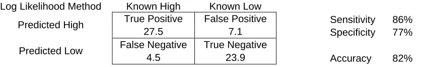
the sequence. The average results of 10 cross validations using log likelihood method can be seen in table 5. Our results demonstrate that 86% of the highly expressed MORFs were correctly classified as high while 71% of lowly expressed MORFs were correctly classified as low. The overall classification managed to obtain an accuracy of 82%. The new measure of codon bias seems to be a better indicator than the CAI metric.

Log Likelihood Method Known High Known Low

Predicted Low

[image:32.612.118.539.220.287.2]

4.5 23.9 Accuracy 82%

Table 5– Classification based on protein expression levels using the log likelihood method. Note that

the specificity of this approach is much higher than the codon adaptation index (Table 3).

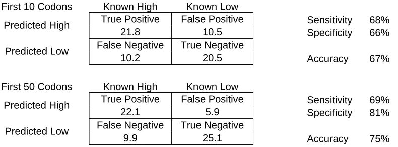
Analyzing the Early Portion of the Transcript

(33)

First 10 Codons Known High Known Low

Predicted Low

10.2 20.5 Accuracy 67% First 50 Codons Known High Known Low

Predicted Low

[image:33.612.123.518.87.233.2]

9.9 25.1 Accuracy 75%

Table 6 – Protein classification using the early codons. The results of classifying sequences based on log

likelihood scores from the first 10 and first 50 codons of MORF sequences.

Our result shows that the log likelihood method performed poorly when only the early portion of the transcript was used. Using the first 10 codons gave an accuracy of 67% and using just the first 50 codons generated an accuracy of 78%.

One reason for these poor results may be the presence of rare codons in clusters. The final score reflects the overall codon profile, not regions of the sequence. A cluster of rare codons might exist for example near position 5. But since the score takes into account all the regions, the effect of this cluster diminishes. Translation is postulated to slow down when the ribosome encounters a region filled with rare codons. The ribosome has to wait for the correct tRNA to enter the site and this occurs less because a rare codon tends to have a lower corresponding tRNA concentration. However, extended periods of ribosome pausing can lead to destabilization of the ribosome complex thus preventing translation.

(34)

reflected through a low log likelihood score while a lack of rare codons would generate a more positive score. Using the sliding window method we scored the entire sequence and obtained the average performance across 10 cross validation runs.

ATG GGT GCT GCC ACT AGG ACG TCG CCG ….

[image:34.612.107.542.149.288.2]

Log likelihood score 0.7 0.8 0.3 –0.2 –0.6 –0.9 ….

Figure 5 – Diagram of sliding window. An example of sliding window using 4 codons was used to assess

clusters of rare codons.

Table 7 shows the results of the log likelihood method using the sliding window model. Here, we only obtained a sensitivity of 70%, specificity of 73% and accuracy of 72%. The relatively low accuracy of our model suggests a lack rare codon clusters in our dataset.

Rare codon cluster Known High Known Low

Predicted Low

[image:34.612.115.510.485.552.2]

9.6 22.6 Accuracy 72%

Table 7– Performance of Log likelihood method using rare codon clusters. Using a sliding window, the

log likelihood score was calculated for windows of 10 codons.

(35)

scoring each codon, we introduced another parameter which immediately classifies the MORF as being a low expressor if the log likelihood score drops below a given threshold (obtained from training dataset). From our training data, we determined that a threshold score of –5 was appropriate. This would mimic the behavior of the ribosome dropping off a transcript that has a consistently poor codon profile.

Using the updated method, we scored the high and low MORFs, scanning each sequence until it reached a cumulative score of –5 and then classifying it. We performed 10 cross validation runs to obtain the results as listed in table 8.

Log likelihood

threshold model Known High Known Low

Predicted Low

[image:35.612.130.524.297.368.2]

5.4 25.1 Accuracy 82%

Table 8 – Performance of Log likelihood method using a threshold cut off value. Here, we used a

threshold value of –5 to immediately classify a sequence as a low MORF. That is, if the cumulative score

for a sequence dropped below –5, we immediately classified the sequence without further scanning the

remainder of the transcript.

The threshold method managed to obtain a sensitivity of 83%, specificity of 81% and an accuracy of 82%. The accuracy of this method is comparable to the log likelihood method when scoring the entire sequence. The consistency between these two scores suggests that it is not the specific presence of individual rare codons but their cumulative effect that affects protein expression levels.

Analysis of Rare Codons

(36)

per 1000 codons. Using the MORF dataset, we identified 25 codons that meet this criterion (table 9). Due to the degeneracy of the genetic code, the number of rare codons varies among different synonymous codon families. In one extreme are the amino acid Asp and Phe where none of the synonymous codons are rare. In the other extreme are the amino acids such Cys and Trp which are always encoded by rare codons. The proportion of synonymous codons that are rare codons can be grouped into several categories. These categories, ranked in descending potential for rare codon use are as follow (Cys, Trp) All rare, (Arg) 5/6 rare, (Leu) 4/6 rare, (Ser) 2/6 rare, (Gly) 3/4 rare, (Val, Pro) 2/4 rare, (His, Ser, Gln) 1/2 rare, (Thr, Ala) 1/4 rare, (Phe, Met, Tyr, Asn, Lys, Asp, Glu) 0 rare. Note that these results are consistent with the previous studies that have used the Codon Usage Database (http://www.kazusa.or.jp/codon/) to identify rare codons. The only exceptions are two codons GCC, GTC which was classified as rare only by Codon Usage Database dataset.

(37)

Acid

Rare

Codon High Morfs Low Morfs All Morfs Amino Acid Rare

Codon High Morfs

Low Morfs

All Morfs Ala GCG 5.31 6.5 5.94 Leu CTC 3.64 5.51 4.63

CTG 8.36 11.5 10.02 Arg CGG 0.81 2.16 1.52 CTT 8.79 12.12 10.55

CGC 1.71 2.9 2.34 CTA 11.76 13.65 12.76 CGA 1.2 3.73 2.54 CGT 6.66 5.73 6.17 Pro CCG 3.22 6.16 4.78 AGG 6.5 11.25 9.01 CCC 5.65 8.05 6.92

Cys TGC 3.33 4.68 4.04 Ser TCG 6.07 9.92 8.11 TGT 7.29 7.24 7.26 AGC 6.96 11.89 9.57

Gln CAG 9.72 14.98 12.5 Thr ACG 5.87 9.49 7.78

Gly GGG 5.44 6.63 6.07 Trp TGG 9.13 9.26 9.2 GGA 8.31 11.88 10.2 GGC 10.81 10.49 10.64 Val GTG 10.51 11.27 10.91 GTA 8.83 12.97 11.02

[image:37.612.110.551.70.397.2]

His CAC 8.07 8 8.04

Table 9– Rare codons with a frequency of less then 13 per 1000 codons. Based on the prevailing

definition of rare codons, we identified 25 such codons in the MORF data set. However, many of these

codons are equally rare in both the high and low MORFs.

(38)

negative codon log value would suggest prevalence in lowly expressed MORFs, while a more positive score indicates prevalence in highly expressed MORF. Since the codon log ratio value for CGA is negative and has a score less than the mean minus one standard deviation, the codon was considered rare. Using this updated definition, we reexamined the codon usage profile to generate a set of new rare codon listed in table 10. The new set of rare codons is compromised of 8 codons which include (Arg) 4/6, (Ser) 2/6 rare, (Pro, Thr) 1/4 rare.

Frequency per 1000 Amino

Acid

Rare

Codon _{High Morfs} _{Low Morfs All Morfs} Arg AGG 6.5 11.25 –0.238

[image:38.612.198.450.271.463.2]

CGA 1.2 3.73 –0.493 CGC 1.71 2.9 –0.229 CGG 0.81 2.16 –0.426 Pro CCG 3.22 6.16 –0.282 Ser AGC 6.96 11.89 –0.233 TCG 6.07 9.92 –0.213 Thr ACG 5.87 9.49 –0.209

Table 10 – Rare codon defined by the new definition. Here, rare codon must have both a frequency of

less than 13 per 1000 codons and a codon log value less than - 0.199.

(39)

Rare Codon per Quartile

Previous analyses have suggested that the early portion of the transcript might be important in determining expression. In fact, the existence of rare codon early within the transcript has been suggested as one of the strongest indicators for poor expression [12]. To test this in our dataset we had to first account for variations in sequence length. In order to accurately model the rare codon distribution, we divided each MORF sequence into quartiles and determined the number of rare codons across quartiles. Figure 6 shows the overall trend in the entire dataset.

Rare codon per quartile

0 1 2 3 4 5 6 7 8

q1 q2 q3 q4

Quartile

Percent of rare codon

[image:39.612.111.551.317.629.2]

High Low

Figure 6 – Rare codon counts per quartile. Comparison of rare codon counts per quartile between high

(blue) and low (red) MORFs. Average length of sequence in each quartile is 273 ± 112. Here, it is obvious

(40)

In the first quartile, we can see that the low expressing group has about twice the number of rare codons compared to the highly expressed group. This gap becomes smaller in the second, third and fourth quartile. Note that the large rare codon differences in the first quartile are consistent with previous findings. However, depending on the sequence length, the early portion of the transcript can be a variable length.

Position Specific Rare Codons

(41)

Comparison of Rare Codon per Position Between The Two Expressing Group

0 1 2 3 4

0 5 10 15 20 25 30 35 40 45 50 55 60 65 70 75 80 85 90 95 100

Codon Positions

Ave Number of Rare Codons

[image:41.612.112.537.72.293.2]

High Low

Figure 7– Positions specific rare codon distribution in the first 100 codon. To assess the position

specific bias, if any, of rare codons, we counted the number of rare codons present in the low and high

MORFs for the first 100 nucleotides of each sequence. The number of rare codons was obtained by

averaging across 10 cross validation runs.

(42)

Rare codons in highly expressed group

-1 0 1 2 3 4

0 5 10 15 20 25 30 35 40 45 50 55 60 65 70 75 80 85 90 95 100

Codon position

A

v

e

n

um

b

e

r

o

f r

a

re

c

odo

[image:42.612.112.535.73.306.2]

ns

Figure 8 – Position specific rare codon in the first 100 codon shown with errors bars. The mean

number of rare codon specific to its positions is averaged across 10 cross validation run. The errors bar

(vertical lines) show one standard deviation away from the mean value.

Positions with Significant Rare Codon Difference

(43)

Position With Significant Difference In The Number of Rare Codons

0 1 2 3 4

4 15 17 19 29 31 39 46 49 54 65 68 71 83 85 93 96

Codon Position

Ave Nu

m of Rare Codons

[image:43.612.112.537.74.286.2]

High Low

Figure 9 – Codon positions exhibiting significant difference in rare codon between the expressing

groups. Codon positions with the most significant difference in rare codon frequencies are shown here.

These codon positions can be used as another parameter in our log likelihood model. That is, we can determine the relative importance of these positions by seeing how well we can classify sequences for protein expression level based on the codons present in these positions. We modified our method to score the sequence only based on these 17 codon positions. The result averaged across 10 cross validation runs is shown in table 11.

Known High Known Low True Positive False Positive Sensitivity 69% Predicted High

Predicted Low

9.9 23.25 Accuracy 72%

Table 11 – Performance of log likelihood method scoring only the 17 codon positions. These 17

positions represent those where the low MORFs in the training set have many more instances of rare

codons than the high MORFs.

[image:43.612.132.510.501.567.2]

(44)

rare codons might not be as significant in determining protein levels as earlier work had suggested.

Maximal Dependence Decomposition (MDD)

In an attempt of identify specific positions influencing expression, an alternative approached was used which utilizes the goodness of fit test. The goal of maximal dependence decomposition (MDD) is to generate a model which captures the most significant dependencies between nucleotide positions [30]. Taking just the first 300 nucleotides of each MORF in our dataset, we calculated the chi–squared score from one position to every other position. The scores are then used to construct a 300 x 300 matrix of chi–squared score. A portion of this matrix can be seen in table 12.

Position j

3 4 5 6 7 8 9 10 3 - 207 11.9 16.9 18.8 19.5 0.71 9.98 4 207 - 24.8 12 9.44 9.53 12.3 14.8 5 11.9 24.8 - 18.5 4.91 8.5 5.38 4.79 6 16.9 12 18.5 - 93.4 16.8 18.3 14.7 7 18.8 9.44 4.91 93.4 - 19.7 14 11.1 8 19.5 9.53 8.5 16.8 19.7 - 3.83 13 9 0.71 12.3 5.38 18.3 14 3.83 - 80.1

Pos

ition

i

[image:44.612.214.446.383.657.2]

10 9.98 14.8 4.79 14.7 11.1 13 80.1 -

Table 12– A portion of the 300 x 300 chi–squared matrix. The complete list can be found on the

(45)

Here, we can see that position 3 (1st nucleotide of a codon) exhibits significant dependence on position 4 (2nd nucleotide of a codon) as signified by the large chi– squared score of 208. Position 6 (1st nucleotide of a codon) is also strongly dependent on its next nucleotide at position 7 (chi–squared score = 93.4). In fact, further analysis revealed an abundance of dependencies occurring between adjacent nucleotides. Note that some level of dependency is expected to occur between the nucleotides of a codon. Normally, it is customary to do an MDD analysis at a higher level, such as at the second order level, which would account for the triplet codon dependencies. However, we had insufficient data to do so. Therefore, we simply eliminated significant positions that are next to each other and focused on non–adjacent codons. Table 13 displays 15 positions which have the most significant chi–squared scores after eliminating neighboring positions.

Position i Position j Nucleotide Codon Nucleotide Codon

[image:45.612.201.447.410.643.2]

Chi– square 7 (3) 39 (14) 37.61 15 (6) 114 (39) 38.6 16 (6) 27 (10) 37.94 36 (13) 119 (40) 32.94 60 (21) 174 (59) 34.97 86 (29) 250 (84) 36.69 95 (32) 152 (51) 33.97 100 (34) 199 (67) 34.49 133 (45) 221 (74) 36.23 137 (46) 217 (73) 33.99 142 (48) 280 (94) 32.59 153 (52) 243 (82) 39.14 171 (58) 264 (89) 32.14 180 (61) 240 (81) 32.7 200 (67) 288 (97) 32.07

Table 13– Significant dependence in nucleotide positions. Nucleotide and codon positions exhibiting

significant dependence between position i and position j in the dataset are displayed. The chi–squared score

(46)

Interestingly, a large number of non–adjacent codons exhibit significant dependencies. The results in table 13 show great density and more complex pattern of dependencies. For example, nucleotide position 153 (3rd nucleotide of codon 52) exhibits dependence on position 243 (3rd nucleotide of codon 82), which is located over 90 bases away. These long range dependencies appear to be occurring throughout the sequences. The most influential position, based on row sums, was nucleotide position 167 (2nd nucleotide of codon 56). When we split on this position, however, we did not obtain any significant dependencies.

Using the log likelihood method, we wished to capture the apparent long–range dependencies of the significant positions and assess their role in possibly influencing protein expression. Once again, we modified the log likelihood method, this time we scored only positions exhibiting strong dependence as determined by MDD and reported in table 14.

Known High Known Low Predicted High True Positive False Positive Sensitivity 69% 22.1 6.5 Specificity 79%

Predicted Low False Negative True Negative

[image:46.612.114.492.433.500.2]

9.9 24.5 Accuracy 74%

Table 14– Performance of log likelihood method scoring dependent positions. We used the MDD

selected significant positions for scoring sequences and obtained much better classification than with the

position specific log likelihood method using rare codons (Table 10).

(47)

DISCUSSION

In this study, we analyzed the intrinsic properties of the coding sequence and its ability to affect protein expression. The MORF library was specifically constructed to eliminate the effects of promoters and regulators on protein expression levels. Yet, expression analysis still detected substantial variation in protein expression which can be classified as high, medium and low. Investigation into the codon usage profiles between the expressing groups also revealed specific preferences in synonymous codon choice. Highly expressed MORFs tend to favor one set of codons while lowly expressed codons favor another. Based on this differential codon bias, we modeled this phenomenon using the codon adaptation index and several variations on a scoring scheme using log likelihood ratios of codon frequencies between high and low MORFs.

(48)

Model Performance Sensitivity Specificity Accuracy

TP FN SN TN FP SP CAI 23.7 8.3 74% 23.9 7.1 77% 76% LL – Threshold of -5 to classify

sequence as a low expressor 26.6 5.4 83% 25.1 5.9 81% 82% LL – Sum of log likelihood ratios

across entire sequence 27.5 4.5 86% 23.9 7.1 77% 82% LL – Only significant positions scored

based on maximal dependence decomposition 22.1 9.9 69% 24.5 6.5 79% 74% LL – First 50 codons scored 22.1 9.9 69% 25.1 5.9 81% 75% LL – Only significant positions based

[image:48.612.106.586.76.304.2]

on position specific rare codons were scored 22.1 9.9 69% 23.25 7.75 75% 72% LL – Scores based on sliding window 22.4 9.6 70% 22.6 8.4 73% 72% LL – First 10 codons scored 21.8 10.2 68% 20.5 10.5 66% 67%

Table 15 – Comparison of various classifier models. The Codon Adaptation Index (CAI) was compared

to a number of log likelihood (LL) variations. The true positive (TP), false negative (FN), true negative

(TN), false positive (FP) was obtained by averaging across 10 cross validation runs. Sensitivity (SN),

specificity (SF) and accuracy was calculated by formula 5, 6 and 7 respectively.

(49)

The early portion of the transcript clearly displays a differential codon usage pattern. Lowly expressed genes have been shown to contain more rare codons than highly expressed in this region (figure 6). The region could potentially play a role in determining expression, but this role does not seem to be a definitive one. While it is necessary to have a good codon usage, this feature alone is not sufficient for classifying protein expression.

Investigation of rare codon clusters using the log likelihood method also generated mixed results. A number of studies have found the clustering of unfavorable codons to interfere with expression. We did not observe this in our S. cerevisiae dataset. The log likelihood metric using a sliding window model only managed to obtain an accuracy of 72%. The fact that the threshold model obtained a higher accuracy than the sliding window model further questions whether rare codon clusters can dramatically affect protein expression on their own.

(50)

decomposition positions. Our analyses suggest that certain positions do wield some influence, but again, these are not on their own sufficient to completely explain observed levels of protein expression.

Investigation into the MORF sequences revealed several key features that seem to be affecting expression. First we observed a distinct codon bias between the expressing groups. Highly expressed MORFs tend to utilize a preferred set of synonymous codons while lowly expressed MORF follow a different set. This differential codon usage profile in S. cerevisiae appears to be strong influence in protein expression. This is evident by the high accuracy achieved through the log likelihood method using the entire sequence and threshold model.

(51)

CONCLUSION

The log likelihood method has been shown to be a good indicator of protein expression in the MORFs dataset. This metric consistently outperformed the codon adaptation index across 10 cross validations runs, achieving a sensitivity of 83%, specificity of 81% and an overall of accuracy 82%. Therefore we concluded that our log likelihood metric is a better classifier than the previously favored codon adaptation index.

The MORF collection library is one of the best libraries of genes and protein expression levels in S. cerevisiae. Analysis of MORFs sequences revealed several key features. The early portions of the transcript have been shown to have a strong bias in codon composition. Rare codons and clusters of rare codons were also found throughout the sequences. Finally, nucleotide and codon positions exhibiting strong dependence have also been identified. However, none of these features appear to be strong enough to influence expression on their own.

(52)

REFERENCES

1. Jana, S., and J. K. Deb. "Strategies for Efficient Production of Heterologous Proteins in Escherichia Coli." Applied Microbiology and Biotechnology 67.3 (2005): 289–98. 2. Gustafsson, C., S. Govindarajan, and J. Minshull. "Codon Bias and Heterologous

Protein Expression." Trends in biotechnology 22.7 (2004): 346–53.

3. Gouy, M., and C. Gautier. "Codon Usage in Bacteria: Correlation with Gene Expressivity." Nucleic acids research 10.22 (1982): 7055–74.

4. Bennetzen, J. L., and B. D. Hall. "Codon Selection in Yeast." The Journal of biological chemistry 257.6 (1982): 3026–31.

5. Friberg, M.,. Limitations of Codon Adaptation Index and Other Coding DNA–Based Features for Prediction of Protein Expression in Saccharomyces Cerevisiae. Vol. 21. New York, NY: John Wiley Sons, 2004.

6. Makrides, S. C. "Strategies for Achieving High–Level Expression of Genes in Escherichia Coli." Microbiological reviews 60.3 (1996): 512–38.

7. A Hoekema, R A Kastelein, M Vasser and H A de Boer. "Codon Replacement in the PGK1 Gene of Saccharomyces Cerevisiae: Experimental Approach to Study the Role of Biased Codon Usage in Gene Expression." Molecular and cellular biology 7.8 (1987): 2914–24.

8. Moriyama, E. N., and J. R. Powell. "Gene Length and Codon Usage Bias in

Drosophila Melanogaster, Saccharomyces Cerevisiae and Escherichia Coli." Nucleic acids research 26.13 (1998): 3188–93.

9. Sharp, P. M., and W. H. Li. "The Codon Adaptation Index––a Measure of Directional Synonymous Codon Usage Bias, and its Potential Applications." Nucleic acids

research 15.3 (1987): 1281–95.

10.Zhang, S. P., G. Zubay, and E. Goldman. "Low–Usage Codons in Escherichia Coli, Yeast, Fruit Fly and Primates." Gene 105.1 (1991): 61–72.

11.Kane, J. F. "Effects of Rare Codon Clusters on High–Level Expression of

(53)

12.Kim, S., and S. B. Lee. "Rare Codon Clusters at 5'–End Influence Heterologous Expression of Archaeal Gene in Escherichia Coli." Protein expression and purification (2006)

13.Batard, Y., et al. "Increasing Expression of P450 and P450–Reductase Proteins from Monocots in Heterologous Systems." Archives of Biochemistry and Biophysics 379.1 (2000): 161–9.

14.Nishikubo, T., et al. "Improved Heterologous Gene Expression in Escherichia Coli by Optimization of the AT–Content of Codons Immediately Downstream of the

Initiation Codon." Journal of Biotechnology 120.4 (2005): 341–6.

15.Kotula, L., and P. J. Curtis. "Evaluation of Foreign Gene Codon Optimization in Yeast: Expression of a Mouse IG Kappa Chain." Bio/technology (Nature Publishing Company) 9.12 (1991): 1386–9.

16.Sharp, P. M., T. M. Tuohy, and K. R. Mosurski. "Codon Usage in Yeast: Cluster Analysis Clearly Differentiates Highly and Lowly Expressed Genes." Nucleic acids research 14.13 (1986): 5125–43.

17.Higgins, S.J. and Hames, B.D. "Protein Expression: A Practical Approach." (1999) 18.Carlini, D. B. "Context–Dependent Codon Bias and Messenger RNA Longevity in

the Yeast Transcriptome." Molecular biology and evolution 22.6 (2005): 1403–11. 19.Gelperin, D. M., et al. "Biochemical and Genetic Analysis of the Yeast Proteome

with a Movable ORF Collection." Genes & development 19.23 (2005): 2816–26. 20.Alexandrov, A., M. R. Martzen, and E. M. Phizicky. "Two Proteins that Form a

Complex are Required for 7–Methylguanosine Modification of Yeast tRNA." RNA (New York, N.Y.) 8.10 (2002): 1253–66.

21.McLachlan, A. D., R. Staden, and D. R. Boswell. "A Method for Measuring the Non– Random Bias of a Codon Usage Table." Nucleic acids research 12.24 (1984): 9567– 75.

(54)

23.Gribskov, M., J. Devereux, and R. R. Burgess. "The Codon Preference Plot: Graphic Analysis of Protein Coding Sequences and Prediction of Gene Expression." Nucleic acids research 12.1 Pt 2 (1984): 539–49.

24.Sato, T., et al. "Codon and Base Biases After the Initiation Codon of the Open Reading Frames in the Escherichia Coli Genome and their Influence on the Translation Efficiency." Journal of Biochemistry 129.6 (2001): 851–60.

25.Ghaemmaghami, S., et al. "Global Analysis of Protein Expression in Yeast." Nature 425.6959 (2003): 737–41.

26.Stanford University Saccharomyces Genome Database November 2006 Online Internet http://www.yeastgenome.org/

27.Cancilla, M. R., A. J. Hillier, and B. E. Davidson. "Lactococcus Lactis

Glyceraldehyde–3–Phosphate Dehydrogenase Gene, Gap: Further Evidence for Strongly Biased Codon Usage in Glycolytic Pathway Genes." Microbiology (Reading, England) 141 (Pt 4).Pt 4 (1995): 1027–36.

28.Freire–Picos, M. A., et al. "Codon Usage in Kluyveromyces Lactis and in Yeast Cytochrome c–Encoding Genes." Gene 139.1 (1994): 43–9.

29.Gharbia, S. E., et al. "Genomic Clusters and Codon Usage in Relation to Gene Expression in Oral Gram–Negative Anaerobes." Anaerobe 1.5 (1995): 239–62. 30.Burge, C., and S. Karlin. "Prediction of Complete Gene Structures in Human

Genomic DNA." Journal of Molecular Biology 268.1 (1997): 78–94. 31.Kozak, M. "An Analysis of Vertebrate mRNA Sequences: Intimations of

Translational Control." The Journal of cell biology 115.4 (1991): 887–903. 32.Kozak, M. "Downstream Secondary Structure Facilitates Recognition of Initiator

(55)

APPENDIX A – Codon Usage Table of 628 MORFs.

Codon amino acid

frequency

per 1000 number Codon amino

acid

frequency

per 1000 number codon amino

acid

frequency

acid

frequency

per 1000 number

TTT F 22.55 (5445) TCT S 22.64 (5465) TAT Y 17.04 (4114) TGT C 7.26 (1753)

TTC F 18.11 (4372) TCC S 14.67 (3541) TAC Y 15.31 (3697) TGC C 4.04 (976)

TTA L 24.00 (5795) TCA S 16.28 (3930) TAA * 1.14 (276) TGA * 0.80 (194)

TTG L 27.92 (6740) TCG S 8.11 (1957) TAG * 0.65 (158) TGG W 9.20 (2221)

CTT L 10.55 (2547) CCT P 13.47 (3252) CAT H 13.44 (3245) CGT R 6.17 (1489)

CTC L 4.63 (1118) CCC P 6.92 (1670) CAC H 8.04 (1940) CGC R 2.34 (565)

CTA L 12.76 (3080) CCA P 19.32 (4663) CAA Q 28.31 (6834) CGA R 2.54 (612)

CTG L 10.02 (2419) CCG P 4.78 (1153) CAG Q 12.50 (3018) CGG R 1.52 (368)

ATT I 27.63 (6670) ACT T 19.97 (4821) AAT N 33.53 (8094) AGT S 13.07 (3156)

ATC I 17.89 (4318) ACC T 13.44 (3244) AAC N 26.83 (6477) AGC S 9.57 (2310)

ATA I 15.42 (3723) ACA T 16.54 (3994) AAA K 41.48 (10013) AGA R 22.69 (5478)

ATG M 20.40 (4924) ACG T 7.78 (1879) AAG K 36.21 (8742) AGG R 9.01 (2175)

GTT V 22.35 (5395) GCT A 23.60 (5697) GAT D 38.64 (9327) GGT G 27.28 (6586)

GTC V 13.10 (3162) GCC A 14.52 (3506) GAC D 22.80 (5503) GGC G 10.64 (2569)

GTA V 11.02 (2660) GCA A 15.45 (3731) GAA E 48.90 (11806) GGA G 10.20 (2462)

(56)

APPENDIX B – Codon Usage Table of 317 Highly Expressed MORFs.

codon amino acid

frequency

acid

frequency

acid

frequency

acid

frequency

per 1000 number

TTT F 21.28 (2420) TCT S 23.26 (2645) TAT Y 15.37 (1748) TGT C 7.29 (829)

TTC F 20.36 (2315) TCC S 15.37 (1748) TAC 16.87 (1918) TGC C 3.33 (379)

TTA L 23.81 (2708) TCA S 12.72 (1446) TAA * 1.30 (148) TGA * 0.76 (86)

(57)

APPENDIX C – Codon Usage Table of 311 Lowly Expressed MORFs.

codon amino acid

frequency

acid

frequency

acid

frequency

acid

frequency

per 1000 number

TTT F 23.69 (3025) TCT S 22.08 (2820) TAT Y 18.53 (2366) TGT C 7.24 (924)

TTC F 16.11 (2057) TCC S 14.04 (1793) TAC Y 13.93 (1779) TGC C 4.68 (597)

TTA L 24.18 (3087) TCA S 19.45 (2484) TAA * 1.00 (128) TGA * 0.85 (108)

(58)

APPENDIX D – Codon Log Ratio Table

Acid Codon _{High Morfs} _{Low Morfs} Log Value

Ala GCG 5.31 6.5 –0.088 GCA 14.53 16.28 –0.049 GCC 18.5 10.98 0.227 GCT 31.1 16.92 0.264 Arg CGA 1.2 3.73 –0.493

CGG 0.81 2.16 –0.426 AGG 6.5 11.25 –0.238 CGC 1.71 2.9 –0.229 AGA 23.69 21.8 0.036 CGT 6.66 5.73 0.065 Asn AAT 25.31 40.85 –0.208

AAC 26.44 27.18 –0.012 Asp GAT 37.98 39.22 –0.014

GAC 25.04 20.79 0.081 Cys TGC 3.33 4.68 –0.148

TGT 7.29 7.24 0.003 Gln CAG 9.72 14.98 –0.188

CAA 29.02 27.68 0.021 Glu GAG 19.4 20.7 –0.028

GAA 53.88 44.47 0.083 Gly GGA 8.31 11.88 –0.155

GGG 5.44 6.63 –0.086 GGC 10.81 10.49 0.013 GGT 36.27 19.27 0.275 His CAT 11.69 15.01 –0.109

CAC 8.07 8 0.004 Ile ATA 10.53 19.78 –0.274

ATT 30.67 24.92 0.090 ATC 21.26 14.88 0.155 Leu CTC 3.64 5.51 –0.180

(59)

Acid Codon _{High Morfs} _{Low Morfs} Log Value

Lys AAA 37.37 45.13 –0.082 AAG 39.99 32.85 0.085 Met ATG 19.91 20.83 –0.020 Phe TTT 21.28 23.69 –0.047 TTC 20.36 16.11 0.102 Pro CCG 3.22 6.16 –0.282

CCC 5.65 8.05 –0.154 CCT 12.7 14.16 –0.047 CCA 21.86 17.05 0.108 Ser AGC 6.96 11.89 –0.233

TCG 6.07 9.92 –0.213 AGT 9.93 15.87 –0.204 TCA 12.72 19.45 –0.184 TCT 23.26 22.08 0.023 TCC 15.37 14.04 0.039 Stop TAG 0.73 0.59 0.092

TGA 0.76 0.85 –0.049 TAA 1.3 1 0.114 Thr ACG 5.87 9.49 –0.209

ACA 13.81 18.98 –0.138 ACT 21.06 19 0.045 ACC 15.22 11.85 0.109 TGG 9.13 9.26 –0.006 Tyr TAT 15.37 18.53 –0.081

TAC 16.87 13.93 0.083 Val GTA 8.83 12.97 –0.167

Theses

Thesis/Dissertation Collections

Analysis of yeast codon usage patterns using the movable ORF collection

Rochester Institute of Technology

RIT Scholar Works

ANALYSIS OF YEAST CODON USAGE PATTERNS USING

Thesis Advisor

Thesis/Dissertation Author Permission

Print Reproduction Permission Granted:

ABSTRACT

LIST OF TABLES

TABLE OF CONTENTS

INTRODUCTION ...1

RESULTS ...20

DISCUSSION ...39

Introduction

Codon Usage and Predicting Protein Expression Levels

A New Way to Analyze Codon Usage and Protein Expression Levels

Codon Usage in S. cerevisiae

MATERIALS AND METHOD

Movable Open Reading Frame (MORF)

Calculating Codon Frequency

Codon Adaptation Index (CAI) Model

Log–Likelihood Model

Score

FILTER PARAMETERS

FILTER PARAMETERS

Sensitivity

Maximal Dependence Decomposition (MDD)

RESULTS

CGC 1.71 2.9 GTG 10.51 11.27

Codon Adaptation Index

as the basis for classification.

Analyzing the Early Portion of the Transcript

ATG GGT GCT GCC ACT AGG ACG TCG CCG ….

Analysis of Rare Codons

Rare Codon per Quartile

Quartile

Position Specific Rare Codons

Rare codons in highly expressed group

Positions with Significant Rare Codon Difference

Maximal Dependence Decomposition (MDD)

DISCUSSION

CONCLUSION

TTT F 22.55 (5445) TCT S 22.64 (5465) TAT Y 17.04 (4114) TGT C 7.26 (1753)

TTT F 21.28 (2420) TCT S 23.26 (2645) TAT Y 15.37 (1748) TGT C 7.29 (829)

TTT F 23.69 (3025) TCT S 22.08 (2820) TAT Y 18.53 (2366) TGT C 7.24 (924)