ABSTRACT
The purpose of this paper is to present a new approach in the concept and implementation of autonomy for autonomous spacecraft. The one true ‘artificial agent’ approach to autonomy requires the spacecraft to interact in a direct manner with the environment through the use of sensors and actuators. Rather than using complex world models, the spacecraft is allowed to exploit the dynamics of its environment for cues as to appropriate actions to take to achieve its mission goals. The particular artificial agent implementation used here has been inspired by studies of biological systems. The so-called ‘cue-deficit’ action selection algorithm considers the spacecraft to be a non-linear dynami-cal system with a number of observable states. Using optimal control theory a set of rules is derived which determine which of a finite repertoire of behaviours the spacecraft will perform. A simple model of a single imaging spacecraft in low polar Earth orbit is used to demonstrate the algorithm.
NOMENCLATURE
b battery charge deficitC cost function
H Pontryagin state function
I inertia matrix
k resource accessibility
m data recording deficit
Q resilience
r resource availability t data transmission deficit u control function
x state vector
λ co-state vector
θ attitude angle vector
θ attitude rate vector
ω angular velocity vector
1.0 INTRODUCTION
The development of autonomy technologies is the key to three vastly important strategic technical challenges facing future spacecraft mis-sions. The reduction of mission operation costs, the continuing return of quality science products through increasingly limited communica-tions bandwidth and the launching of a new era of solar system explo-ration, beyond reconnaissance, characterised by sustained presence and in depth scientific studies. New deep space missions, coupled with the challenge to do things ‘faster, better, cheaper’ have highlighted the need for increasingly more autonomous spacecraft and rovers. Spacecraft autonomy will bring significant advantages by improving
Autonomous behavioural algorithm
for space applications
G. Radice and C. R. McInnes
Department of Aerospace Engineering Glasgow University
Glasgow, UK
resource management, increasing fault tolerance and simplifying payload operations. Also, when considering the communication delays in deep space missions, the requirement for autonomy becomes clear. Ground stations and controllers will not be able to communicate and control distant spacecraft in real-time to guarantee precision and safety. There is a need therefore to provide autonomous and semi-autonomous computational capabilities to enable further deep space missions.
One approach to autonomy is concerned with the modelling and building of adaptive autonomous agents, which are systems that inhabit a dynamic, unpredictable environment in which they try to sat-isfy a set of goals. This behaviour oriented approach is appropriate for the class of problems that will face the new generation of micro-satel-lites currently under development for Earth monitoring and interplane-tary missions. These missions will require a high degree of autonomy to meet stringent cost and performance goals. An autonomous micro-spacecraft has multiple integrated tasks such as navigation, battery charging, etc. Similarly neural network, fuzzy logic and expert sys-tems, although successful in some terrestrial fields, such as camera focusing, automobile cruise controls and subway automation, are extremely difficult to validate to ensure the survival of the spacecraft and are software intensive. In contrast recent developments in Artificial Agents borrow heavily from ethology where the agents respond directly to environmental stimuli. The satellites are situated in their environment, orbiting a planet, and connected to its problem domain directly through sensors and actuators. It then has to monitor the environment and determine in isolation what the next problem or goal to be addressed is.
In the approach presented in this report such an artificial agent is proposed that provides a method for action selection that balances the demands of the satellite users – gathering or transmitting data – and the actions necessary to guarantee the survival of the spacecraft – charging the battery and thermal control. The spacecraft is modelled as a non-linear dynamic system with a state space consisting of key inter-nal parameters such as battery charge, memory level and interinter-nal tem-perature. The state space will have a set of lethal limits that define the useful operating domain. A finite repertoire of behaviours is then used to generate a set of actions to control the internal dynamics of the spacecraft. A cost function, which provides the measure of the devia-tion of the spacecraft from its normal equilibrium state space operating point is then generated. Applying Pontryagin’s maximum principle from optimal control theory we obtain a set of optimal action selection rules. The action selection algorithm must then maintain this equilib-rium in the presence of perturbations due to the spacecraft’s own behaviour or from environmental change. For example switching on the heater during eclipse will maintain the internal temperature level, but at the same time drain the battery charge.
2.0 THE AGENT AS A STATE SPACE
The state space model for agents was proposed by Sibly and McFarland(1,2)and further developed by McFarland and Houston(3).
Within this framework the agent is characterised as possessing a minimal set of internal variables that can completely describe its state. In such a description of a biological system we could possibly identify hunger, thirst, temperature, hormone level, etc, as essential physiological state variables. The first to develop this model for a spacecraft was Gillies et al. who identified three state variables as being essential: energy, measured through battery level, internal temperature and memory level(4). These variables sit within an
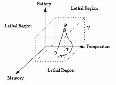
Euclidean vector space with the states as its orthogonal axes as shown in Fig. 1.
Within this space there will be regions that the satellite can physi-cally never encounter, for instance negative memory or negative bat-tery level, and regions, that should the satellite cross into, it would cease to function, such as below the lower or above the upper possi-ble operating temperatures. The boundaries that separate the regions that are fatal to the satellite from those that are not are called lethal limits. The task of the spacecraft within such a model is therefore to maintain the homeostasis (equilibrium) of its state variables under the perturbation of its own behaviour, and the environment’s impact on its resources. For example during eclipse the satellite must acti-vate the heater to stay above the lower lethal temperature, while also draining the battery. In the robotics literature each axis is associated with a specific task the agent has to perform(5-7). However this is not
the case for the spacecraft model. The temperature axis bounds the operational limits for the different subsystems, but is not directly part of the action selection algorithm.
The spacecraft will be able to perform useful work to sustain its viability, by either obtaining images through a payload camera, or gathering data through some appropriate payload instrument, and then storing the data on a hardware device, or downloading, by means of a transmitter, the recorded data to an Earth ground station. Both activities do however require a certain amount of energy to be consumed, draining the battery level. To replenish its energy source the spacecraft must point its solar array towards the Sun, thus recharging the depleted battery. We can see therefore that the space-craft is subjected to three different types of behaviour: target point-ing, ground station pointpoint-ing, and Sun pointing. The temperature seems to bear no importance within the state space since it is not directly related to any particular behaviour. However, it has to be noted that temperature plays a fundamental role in space mission design. All hardware devices work within well-defined temperature limits. It is therefore vital for the mission’s success that the internal temperature is kept within a predefined range to ensure that all sub-systems function properly. The spacecraft is therefore equipped with a heater, which automatically switches on when the temperature reaches a certain lower limit; clearly this requires a certain amount of energy. The temperature therefore is not linked directly to a behaviour, but indirectly affects the spacecraft’s behaviour selection.
3.0 THE OPTIMIALITY CRITERION
It has been shown that the spacecraft’s state can be represented in an n-dimensional space. The state can be thought of as a specification of the value of n variables, where nis large enough to characterise the satellite. The model incorporates a very simple relationship between behaviour and state. It is assumed that when the spacecraft is perform-ing activity ui, the rate of change of the state xi (i = 1-n) is given by:
This means that activity ui, has consequences only along axis xi. The value of riin this model represents the ‘return’ the satellite gets from performing activity ui mediated through a constant parameter ci which links the sensitivity of a variable in relation to an activity.
i i i
i r cu
[image:2.612.56.259.79.228.2]x& =− =− . . . (1)
Figure 1. An example of a possible three-dimensional state space with local origin O. The current state is indicated by the vector P. The
It seems reasonable to assume that the risk of failure, must increase steeply the nearer a state variable is to its lethal boundary. For exam-ple it is obviously dangerous to allow the battery charge to approach lethal levels if a future energy supply is not guaranteed. This sug-gests a cost function of the form:
C(x) ∝x2
The choice of a quadratic function has been made for mathematical simplicity, although clearly any convex function may be used(8). It
has to be noted that the cost function has the desirable property that the cost of possessing any particular deficit increases more rapidly the further away from the homeostatic equilibrium point the satel-lite’s variable lies. When more than one state is being considered, some assessment of the total cost C(x) must be made. If C(x) can be represented as the sum of the cost associated with each xiin x(i= 1-3), then C(x) is said to be separable. This means that the risk associ-ated with the value of one variable is independent of the values of the other variables. So the cost C(x) of being in state z is a weighted sum of the squares of the displacements that constitute x. For exam-ple if x= [x1, x2, x3] then:
C(x) =
where the weighting parameters Qi(i= 1-3) are referred to as the
resilience of the state variable(9). The optimality criterion then
amounts to requiring the spacecraft to spend its time in such a way that the displacements from the homoestatic position results in the smallest possible cost.
To complete the specification of the optimisation problem we then have to resort to Equation (1) to link the satellite’s behaviour to con-sequences for its state. If during some time span the duration of time spent performing activity uiis di then the total consequence of such a
behaviour for axis xiwill be diri. In other words if xibegan at a value
xi(0), its value at the end of the time span considered xi(T) will be given by xi(T) = xi(0) – diri. Therefore at the end of the time span considered the state of the spacecraft will have resulted in a deficit for that axis. As will be seen diplays a fundamental role in the action selection algorithm
3.1 Dynamic optimisation
We will now consider dynamic problems, in which any action taken at any given time has consequences, which are evaluated over some period of time into the future. In this case the problem is to look at the cost associated with different paths through some state space. The optimal solution will be the one along which the total accumu-lated cost is least. Finding this total cost involves the mathematical operation of integration.
The optimal control problem can now be defined. We have an objective function C(x, u, t) dependant on the state variable x, and the behavioural control u. The aim is to move the system, to a speci-fied state or for a specispeci-fied amount of time, such that the integral of the objective function is minimised. A technique that is applicable in such cases was developed by Pontryagin in the 1950s(10). Pontryagin
approached the optimal control problem by defining a state function called the Pontryagin (also know as Hamiltonian) function denoted by H. Pontryagin’s maximum’s principle states that the problem of finding the path of least cost is equivalent to the more direct problem of instantaneously maximising the function H – the principle can also be considered as an instantaneous minimisation.
A constraint is however introduced by the method itself as the dynamic problem of optimal control must represent the fact that the state variable xand the control variable u that constitutes the instan-taneous cost function cannot be varied independently. The reason for the dependence is the fact that ucontrols x, the nature of this control being given by the system equation –Equation (1).
Pontryagin’s function can therefore be thought of as the gradient of the cost functional, that is to say Hindicates how cost varies with
a chosen control at any given position of time. Let us now sum up
the principle: In order to minimise the total cost , the control
the control law u must be chosen in such a way as to instantaneously maximise the Pontryagin function:
where C(x, u, t) is the objective function giving the total cost, ƒ (x, u, t) represents the system equation. Here λrepresents the change in total future cost along the optimal trajectory that results from a small change in state and is called the costate vector. It is, in effect, a set of Lagrange multipliers, introduced to satisfy the system equation con-straint. The rate of change of both the state and costate vectors are then given by the following equations(11):
This formulation will be used later to determine the spacecraft’s optimal behaviour.
3.2 Availability and accessibility
Two parameters, the availabilityrand the accessibility kmodel the resources in the environment. This duality may seem arbitrary, andr and kshould be united into one single variable. However, these two parameters provide a powerful way with which to consider the envi-ronment. The availability is associated with the density of the resource in the environment. The accessibility is associated with the ease with which an agent can obtain the resource through its own behaviour. Applying these definitions to the spacecraft problem allows us to assess the environmental resources at hand for the spacecraft. The availability and accessibility will be associated with the different behaviours the spacecraft is capable of performing. Charging the battery, recording and transmitting data, will therefore all have an assigned accessibility and availability. The spacecraft is equipped with sensors – Sun sensor, and GPS – that determine the availability riof any resource (i= 1-n). For example when the satel-lite detects, via its Sun sensor, that it is in sunlight rsun= 1, while we will have rsun= 0 if the satellite is in the eclipsed arc of its orbit. The ground station availability will be 0 < rground station≤1 when the satel-lite detects through a global positioning system or up-link signal, that the ground station is present, otherwise rground station = 0. Similarly if the satellite is in sight of the target area 0 < rtarget≤1 and rtarget= 0 if not. The rate at which the satellite can perform a certain task is modelled by the accessibility ki(i= 1-n) and is associated
with the ease with which the spacecraft can obtain a resource through its behaviour. For example the rate ksunat which the satellite can charge the battery by pointing towards the Sun is the maximum array power output. If the solar array is damaged then ksunis low-ered: for example if 50% of the array fails at t = tfailure, then ksun(tfailure) = 0⋅5ksun(tlaunch). Similarly we will have kgroundstation, and ktarget which are defined by hardware constraints before launch and determined by the maximum data rates for acquiring and down-link-ing data. Should the satellite suffer an antenna, transmitter or pay-load instrument failure, these parameters would be lowered accordingly.
3.3 Optimal behaviour
We now have all the tools to determine the optimal behaviour the agent will perform at any given time. The solution obtained from Pontryagin’s maximum principle (the optimal behaviour) depends on the conditions constraining the satellite’s behaviour(8). There are four
. . . (2)
. . . (3)
. . . (5)
. . . (6) . . . (4)
3 2 3 2 2 2 1 2 1 + + Q x Q x Q x
∫
= T t t x,u,t C 0 )d ( ) , ( ) , ( T t x,u C t x,u fH= λλ −
important constraints that need to be considered:
1. The impossibility of performing behaviour at a negative rate implies that ui(t)≥0.
2. Behaviours are rate limited, so that the agent cannot work faster than some limiting rate defined by the accessibility ki, therefore
ui≤ki.
3. The rate of performing a behaviour is defined by , for availability riwhere is the rate of change of the state xi (i= 1-n). 4. The satellite can perform only one behaviour at a time. For exam-ple, if the spacecraft is pointing towards the Sun for battery charging it cannot downlink to the ground station or activate the payload.
This last point is worth looking at more closely. Let us consider the case of an animal which allocates a proportion of time s to feeding; then a proportion (1-s) will be available for drinking. This, assumes that drinking and feeding are the only two behaviours that the animal performs. If feeding occurs at a maximum rate, then the rate of feed-ing at that stage is sk1. In general, considering condition two we can
say that u1≤sk1and u2 ≤(1-s)k2, which can be expressed, taking into
account condition one as:
The optimal behaviour therefore requires the controls uito maximise
Hsubject to the constraints 1-4 introduced previously. The optimal control strategy is to set u1= k1and u2= 0 if the current state of the
agent is to the left of the switching line and u1= 0 and u2= k2if the
current state is to the right. Therefore we will have the two following situations:
Perform behaviour 1 at rate k1if λ1r1k1> λ2r2k2
Perform behaviour 2 at rate k2if λ2r2k2> λ1r1k1
Thus the optimal trajectory heads towards the switching line – where
λ1r1k1= λ1r1k1– and then follows it to the origin. Moreover if we
look at how we defined the Pontryagin function, Equation (10), and how the costate vector λis defined, Equation (8), we can introduce a new parameter called deficit which is defined as(12):
and therefore if we consider the two competing behaviours as eating and drinking we will have:
Eat at rate k1if d1r1k1> d2r2k2
Drink at rate k2if d2r2k2> d1r1k1
This solution combines the agent’s state with the parameters that describe the environment. The interesting property to note is that the structure of the rule does not change depending on the type of cost function chosen. The cost function acts simply as a scaling factor to the state variables. We can therefore say that the optimal behaviour is to perform an activity at the maximum rate at which it is available and a choice made between behaviours. Therefore, the choice between feeding and drinking should be made according to whether the product of deficit ×availability ×accessibility is greater for food or water. Several examples of this motivational behaviour have been studied in the animal kingdom(13-16). This switching rule now forms
the basis for the spacecraft action selection algorithm.
3.4 Satellite action selection algorithm
We can now apply what we have introduced previously to the case of an autonomous agent, and in particular to the case of an autonomous satellite. For a spacecraft possessing the three essential state variables discussed earlier: battery charge, memory level and internal temperature, the cost function has been determined to have the following expression(4).
C= b2+ t2+ m2
Where brepresents the battery charge deficit, trepresents the data transmission deficit and m represents the recording deficit. A deficit is defined as being the magnitude of the difference between some current state variable and its nominal equilibrium value. The deficits have the following expression:
where the subscript cidentifies the current value of a state variable – b, battery charge, and m, memory level – and the subscripts maxand min, identify the upper and lower lethal values for the state variable. It can be noted how the deficit for the battery charge increases as the value of the current battery charge decreases. Similarly the deficit for recording data is greatest when the current available memory space, identified by mc, is zero, and decreases as the storage device
fills with recorded data. Opposite is the behaviour of the transmis-sion deficit t, which is highest when the memory is full, and decreases as data is down-linked to the ground station freeing up storage space. Essentially, the state variable deficits determine how far away from the origin that state variable is. Finally, it must be noted that a quadratic cost function has the desirable property that the cost of possessing any particular deficit increases more rapidly, than linearly, the further away from the homeostatic equilibrium point the spacecraft’s variable lies. This is important because the closer the spacecraft is to a lethal limit, the more likely it is that it will suffer a failure and cease to operate.
The system equations, which link the rate of change of a state variable with a behaviour for the satellite are:
with the constraint on the behaviours given by:
To ensure its survival, the spacecraft must never drain its battery below the lower lethal limit. The satellite energy deficit b, is the measure of how much the batteries have discharged. Pointing the solar panels towards the Sun and charging the battery reduces this deficit. The spacecraft must also produce useful work, by recording data from its payload and transmitting it back to Earth. The payload will be associated with a work deficit composed of a recording deficit m, and a transmitting to Earth ground station deficit t. By storing data, the spacecraft may reduce the recording deficit, while downloading data back to Earth will reduce the transmission deficit. It has been shown earlier that the behaviour to be performed by the spacecraft is the one associated with the highest drkproduct. In this formulation the deficits from the state variables combine with stim-uli from the environment to determine a behavioural sequence. The stimuli are considered to be a cue to resources that will have conse-quences to the agent’s state variables.
The decision to perform a particular behaviour is made by calcu-lating the tendencies to perform all the various activities the space-craft may exhibit and choosing the behaviour that possesses the highest tendency as explained in Section 3.3. Empirical evidence 1
0
2 2
1
1+ ≤
≤
k u k u
. . . (7)
. . . (9)
. . . (10a)
. . . (10b)
. . . (10c)
. . . (8)
min max c max b b b b b= − − max c max m m m
m= −
max c m m t= i i= x d ∂ ∂C
. . . (11a)
. . . (11b)
. . . (11c)
. . . (12) s
sunu
r b&=−
t transmitu
r t&=−
r recordu
r m&=−
1
0≤ ≤
record r transmit t sun s k u + k u + k u i i i ru
that this occurs in animals has been discussed at length(17-18). In
addition, the cost function model predicts that such a multiplicative combination rule, when applied to the deficit and cue, should gen-erate optimal behaviour sequencing. We can therefore finally sum-marise the problem of optimal control for the spacecraft as:
behaviour ⇒Max[deficit × availability × accessibility]. Max[b× rsun×ksun] ⇒Charge the battery
Max[m× rtarget× ktarget] ⇒ Record data
Max[t× rground station× kground station] ⇒ Transmit to Earth ground station
The satellite selects the optimal behaviour by computing the various deficits, taking environmental cues to assess availability and accessi-bility of the resources and finally calculating the drkproduct associ-ated with each behaviour. The optimal behaviour at any time is therefore the one which yields the highest of the above products. This algorithm also shows a degree of opportunism, because it con-siders environmental factors together with internal deficits. For example even if the battery deficit is low and the work deficit is high, the satellite may still opt to charge the batteries if sunlight is available and cues for doing work – visibility of ground station or target area – are low. Such opportunism is one of the major benefits of this algorithm and it is difficult, if not impossible, to code into conventional artificial intelligence engines. Another significant advantage of such a method is that the spacecraft measures environ-mental parameters (such as the presence of sunlight or ground sta-tion) and internal parameters (such as battery charge and memory level) so that complex models of the environment are not required to select the appropriate behaviour. Also, it is not necessary to have complex models of the spacecraft and its internal subsystems. If we consider the battery charge as an example, the model used for it is not directly relevant to the performance of the action selection algo-rithm; the algorithm uses the direct measure of battery charge rather than a model of the battery. Therefore, we can expect that the model-ling of more complex and numerous spacecraft subsystems will not change the qualitative behaviour of the algorithm. This method how-ever may easily incorporate additional tasks which will either form part of the action selection process, or which can be scheduled at a particular time by setting the drkproduct to equal unity at a fixed time. Adding extra tasks is straightforward; each new behaviour will be given a deficit, availability and accessibility. The resulting behav-iour will always be the one with the highest drkproduct.
4.0 CASE STUDY
The satellite will operate in different orbits and is considered to have three rotational degrees of freedom that can be controlled by reaction wheels. The spacecraft is modelled as a cube and to provide pointing constraints the antenna, camera and solar panel are placed on differ-ent sides of the spacecraft. The electrical power system consists of a
solar array, battery and several electrical loads. The payload is a camera that records at a steady rate when active and a radio transmit-ter to broadcast data to the ground station. The individual subsys-tems are coupled together: switching the transmitter on drains the battery and reduces the amount of stored data. The spacecraft is con-trolled by switching the camera, the transmitter and an internal heater on or off, and commanding the attitude control subsystem to track one of the three targets – Sun, Earth ground station and Earth target – by activating the reaction wheels. The spacecraft has an internal heater which may be switched on or off independently of what other task the spacecraft may be performing; the heater is auto-matically activated when the temperature drops below a certain threshold value fixed at 240K and is not commanded by an action selection algorithm. The heater however drains the battery, and therefore indirectly influences the action selection process. The spacecraft selects the optimum behaviour at any time by evaluating the deficits of the state variables – battery and memory level – assessing the availability and accessibility of the environmental resources – Earth ground station, Sun and Earth target – and finally computing the drkproduct. The spacecraft will switch between dif-ferent behaviours when the difference between two drkproducts sur-passes a fixed threshold. The user selects the ground station and target co-ordinates (azimuth and elevation) within the appropriate blocks. Other parameters that can be defined by the user are the orbital parameters – apogee, perigee, inclination, ascending node and perigee argument – the inertia moments(11-13)of the spacecraft and
the free parameters αiand βi(i= 1-3) which influence the pointing
control algorithm; all these variables can be modified from within the satellite block. Finally the user can change the state variables lethal limits – internal temperature, memory space and battery power – within the action selection block. In Fig. 2 we can see the complete Simulink model.
To test the action selection algorithm the spacecraft is inserted into a low Earth polar orbit. The orbit is circular with a 500km alti-tude, and an inclination of 85⋅95°. There is one single ground station present placed at 57⋅3° latitude, the latitude of Glasgow. There are also six different target areas situated at 80° latitude and evenly spaced in longitude between each other. The simulation runs for just over 90 orbital periods, which equates approximately to six mission days. In Figs 3-9 we can see the results of this.
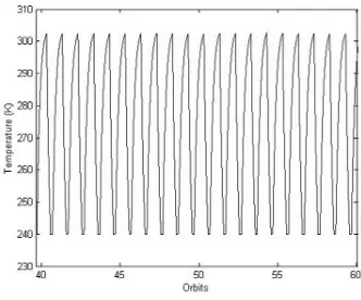
As can be noted from Figs 3-5 the temperature oscillates as the spacecraft goes in and out of the eclipse part of the orbit – the tem-perature increases while the spacecraft is in direct sunlight, while the temperature decreases while the spacecraft is in eclipse. When the internal temperature reaches the threshold value of 240K the heater automatically switches on to maintain the temperature above the minimum lethal level. The threshold value is selected by the user and is quite arbitrary although this value is linked to different space-craft components which have an optimal operational range. It can also be noted how the spacecraft charges the battery when in direct . . . (13a)
. . . (13b)
[image:5.612.350.516.78.216.2] [image:5.612.36.283.80.195.2]. . . (13c) Figure 2. Complete simulink model.
sunlight by pointing the side mounted with the solar array towards the Sun. It is interesting to note what happens during the eclipse phase of the orbit to the battery charge level. We can see different slopes as the battery charge level decreases. This is due at first because the transmitter or payload are active; when either is opera-tional there is a demand on the battery for their activation. After that, there is a period during which the transmitter or payload are not active and the discharge in the battery level proceeds at a lower rate. When the heater is then turned on to maintain the internal tempera-ture, the battery is discharged at an increased rate.
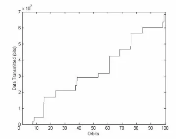
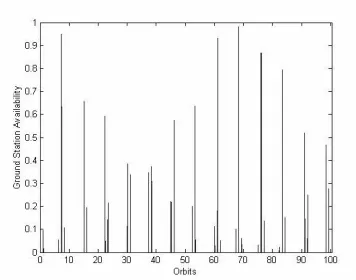
Several interesting comments can be made by looking at Figs 6 and 7. First of all it should be noted that the spacecraft does not fly over the six different target areas during one orbit period. Also the target availability varies during each orbit as previously. There are then two interesting differences that we can highlight when looking at the stored data and the target availability. When the availability of the resource is high the spacecraft records significant data. However when the availability of the target area is low the spacecraft may opt not to image as highlighted by the amount of data stored in the memory remaining constant. This is because the spacecraft may have more pressing needs; i.e. charging the battery or downloading recorded data, or because recording data during a low availability flyby is not an efficient activity from an energetic point of view. Similar considerations can be made by looking at Figs 8 and 9. Again the spacecraft does not see the ground station during each orbit, and it actually goes approximately five orbits without ever passing over it. The non-periodic nature of the ground station avail-ability and target availavail-ability is due to the fact that the orbit period of the spacecraft in a 500km circular orbit is 94⋅62mins, and therefore not repeatable during the 24hr rotation period of the Earth. We can see how, when the ground station has a good availability the space-craft transmits significant data. On the other hand when the ground station availability is poor there is not much data transmitted back to Earth.
4.0 CONCLUSIONS
[image:6.612.64.247.71.731.2] [image:6.612.341.520.80.222.2]We have introduced a scheme for sequencing tasks on a spacecraft. The action selection algorithm is easily implemented by virtue of its computational simplicity. Moreover, the strategy is derived from optimal control theory. The model is however somewhat simplified, and an actual spacecraft may have several more operational tasks that may be autonomously controlled or be scheduled or com-manded by ground control. This method however may easily incor-porate additional tasks which will either form part of the action selection process, or which can be scheduled at a particular time by setting the drkproduct to equal unity at a fixed time. Adding extra tasks is straightforward; each new behaviour will be given a deficit, Figure 5. Sun availability.
Figure 4. Battery charge.
[image:6.612.66.250.83.313.2]Figure 7. Target availability. Figure 6. Stored data.
[image:6.612.72.240.405.737.2]availability and accessibility. The resulting behaviour will always be the one with the highest drkproduct. A significant advantage of such a method is that the spacecraft measures environmental para-meters (such as the presence of sunlight or ground station) and internal parameters (such as battery charge and memory level). Complex models of the environment are not required to select the appropriate behaviour. Also it is not necessary to have complex models of the spacecraft components and subsystems. If we con-sider the battery charge as an example, the model used for it is not directly relevant to the performance of the action selection algo-rithm; the algorithm uses the measure of the battery charge rather than using a model of the battery charge. Therefore we can expect that the modelling of more complex and numerous spacecraft sub-systems will not change the qualitative behaviour of the algorithm. The study of such a method can be extended to a constellation of satellites, in which the individual spacecraft co-operate with each other. The co-operation may be as simple as passing data to each other when the memory level is full and the ground station is not available, or as complex as having one master spacecraft command-ing the other slave spacecraft in the constellation. The method, because of its computational simplicity, can also be easily applied to planetary rovers and future ‘satellites-on-a-chip’, where the algo-rithm and behaviours can be hard-wired into the spacecraft.
REFERENCES
1. SIBLY, R.M. ANDMCFARLAND, D.J. A State Space Approach to Motivation, Motivational Control System Analysis, 1974, Academic Press. 2. MCFARLAND, D.J. ANDSIBLY, R.M. The Behavioural Final
Common Path, Philosophical Transactions of the Royal Society, (Series B), 1975, 270, pp 265-293.
3. MCFARLAND, D.J. ANDHOUSTON, A.I.Quantitative Ethology: The State Space Approach, 1981, Pitman.
4. GILLIES, E.A., JOHNSTON, A.G.Y. ANDMCINNESC.R. Action selection algorithms for autonomous micro-spacecraft,J Guidance
Navigation and Control, 1999, 22, (6), pp 914-916.
5. BLUMBERG, B. Action-selection in Hamsterdam: lessons from ethol-ogy, From animals to animats 3: Third international conference on the
simula-tion of adaptive behaviour, 1994, Brighton, UK. 6. STEELS, L. A case study in the behaviour-oriented design of
autonomous agents, From animals to animats 3: third international confer-ence on the simulation of adaptive behaviour, 1994, Brighton, UK. 7. SPIER, E. ANDMCFARLAND, D.J. A finer-grained motivational
model of behaviour sequencing, From animals to animats 4: Fourth interna-tional conference on the simulation of adaptive behaviour, 1996, Boston,
MA.
8. SIBLY, R.M. ANDMCFARLAND, D.J. On the fitness of behaviour sequences, The American Naturalist, 1976, 110, (974), pp 601-617.
9. HOUSTON, A.I. ANDMCFARLAND, D.J. Behavioural Resilience and its Relation to Demand Functions, Limits to Action: The Allocation of
[image:7.612.66.244.78.218.2]Individual Behaviour, 1980, pp 177-203. Figure 9. Ground station availability.
10. PONTRYAGIN, L.S., BOLTYANSKII, V.G., GAMKRELIDZE, R.V. AND
MISHCHENKO, E.F. The Mathematical Theory of Optimal Processes, 1962, John Wiley and Sons, New York.
11. DIXIT, A.K.Optimization in Economic Theory,1976, Oxford University Press.
12. ELGERD, O.Control Systems Theory, 1967, McGraw-Hill, New York. 13. BOLLES, R.C. Theory of Motivation, 1967, Harper and Row, New York.
14. SCHOENER, T.W. Theory of feeding strategies,Annual review of ecolog-ical systems,1971, 2, pp 369-404.
15. MCCLEERY, R.H. On satiation vurves, Animal Behaviour, 1978, 25, pp
1005-1015.
16. Krebs, J.R. Behavioural Aspects of Predation, Perspectives in Ethology, 1973, pp 73-111, Plenum Press, New York.
17. BAERENDS, G.P., BROWERR. ANDWATERBOLKH.T. Ethological studies of Lebistes Reticulatus (Peters). 1. An analysis of the male courtship patter, Behaviour, 1955, 8, pp 249-334.