Stock Prices and Monetary Policy. CEPS Working Document No. 304, September 2008

S

TOCK

P

RICES AND

M

ONETARY

P

OLICY

CEPS Working Document No. 304/September 2008

Paul De Grauwe

The question of whether central banks should target stock prices so as to prevent bubbles and crashes from occurring has been hotly debated. We analyse this question using a behavioural macroeconomic model. This model generates bubbles and crashes. We analyse how ‘leaning against the wind’ strategies, which aim to reduce the volatility of stock prices, can help in reducing volatility of output and inflation. We find that such policies can be effective in reducing macroeconomic volatility, thereby improving the trade-off between output and inflation variability. The strength of this result, however, depends on the degree of credibility of the inflation-targeting regime. In the absence of such credibility, policies aiming at stabilising stock prices do not stabilise output and inflation.

CEPS Working Documents are intended to give an indication of work being conducted within CEPS research programmes and to stimulate reactions from other experts in the field. Unless otherwise indicated, the views expressed are attributable only to the author in a personal capacity and not to any institution with which he is associated.

ISBN-13: 978-92-9079-819-4

1. Introduction ... 1

2. A behavioral macroeconomic model ... 2

2.1 The basic model ... 3

2.2 Introducing asset prices ... 3

2.3 Expectations formation: forecasting output ... 5

2.4 Expectations formation: forecasting inflation... 7

2.5 Calibrating the model... 8

3.

‘

4. Inflation targeting and macroeconomic stability ... 11

5. The tradeoff between output and inflation variability ... 13

6. Conclusion... 16

References ... 17

| 1

CEPS Working Document No. 304/September 2008

P

AUL

D

E

G

RAUWE

1. Introduction

The question of whether central banks should react to stock price developments has been hotly debated. It is fair to state that there are two schools of thought on this issue. The first one, which is well represented by Bernanke & Gertler (2001), Schwartz (2002), and Greenspan (2007), argues that central banks should not use the interest rate to influence stock prices. The main

arguments advanced by this school of thought are, first, that it is difficult to identify bubbles ex

ante, (and it only makes sense to intervene if stock prices are on a bubble path, i.e. if they

clearly deviate from underlying fundamentals).1 The second argument is that even if a bubble

can be identified ex ante, using the interest rate is ineffective to burst a bubble. All the central

bank can do is to limit the damage once the bubble bursts. This school of thought also stresses that by keeping the rate of inflation low, the central bank contributes to creating an environment of sustainable growth in which bubbles are less likely to emerge.

The second school of thought takes the opposite view (see Smets, 1997, Ceccetti et al., 2002, Borio & White, 2004, Bordo & Jeanne, 2002 and Roubini, 2006). Stock prices are often subject to bubbles and crashes. These can have strong pro-cyclical effects and can also affect the stability of financial markets. Since central banks are responsible for financial stability they should monitor asset prices and try to prevent the emergence of bubbles (that invariably lead to crashes). In this view the use of the interest rate is seen as effective in preventing bubbles from

emerging.2 Few economists from this school will argue that the central bank should target a

particular value of the stock price (in the same way as it targets an inflation rate). Instead many will argue that a strategy of ‘leaning against the wind’ may be useful to reduce too strong movements in stock prices.

In this paper we analyze the question of whether central banks should try to influence stock prices using their interest rate policy. We will do this in the context of a behavioural macroeconomic model as developed in De Grauwe (2008). (For similar models see Branch & Evans (2006) and Brazier, et al. (2006)). Thus we depart from rational expectations and their implementation in the currently fashionable DSGE-models. The reason why we depart from this modelling approach is double. First, DSGE-models make extremely strong informational assumptions, i.e. agents are assumed to understand the structure of the underlying model. This follows directly from the rational expectations assumption which requires agents to use the underlying model structure to make forecasts. The scientific evidence from other sciences

∗

The author is Professor of Economics at the University of Leuven and Associate Senior Fellow at CEPS. A shorter version of this paper is being published simultaneously in the CEPS Policy Brief series (No. 171).

1

An extreme version of this school of thought denies the existence of bubbles altogether. In this view financial markets are efficient and thus stock prices always reflect the best available information. Since central banks do not posses better information than markets, it makes no sense for them to try to influence stock prices.

2

(psychology, brain sciences) casts doubts about the plausibility of this assumption. It is no exaggeration to say that there is now strong evidence that individual agents suffer from deep cognitive problems limiting their capacity to understand and to process the complexity of the information they receive. Many anomalies that challenge the rational expectations assumption were discovered (see Thaler, 1994, for spirited discussions of these anomalies; see also Camerer & Lovallo, 1999, Read & van Leeuwen, 1998, and Della Vigna, 2007).

The second reason why we depart from DSGE-modelling is that in these models there is no room for bubbles and crashes. Markets are always efficient, so that asset prices reflect underlying fundamentals. Thus central banks cannot improve welfare by guiding asset prices to other values than those produced by efficient markets. In a way it can be said that DSGE-models are not the appropriate tools to study the issue of whether central banks should try to prick asset bubbles, as such bubbles cannot occur in these models.

In our modelling approach we will take the view that agents face cognitive problems in understanding and processing information. As a result, they use simple rules (‘heuristics’) to guide their behaviour (see Gabaix et al., 2006). They do this not because they are irrational, but rather because the complexity of the world is overwhelming. In a way it can be said that using heuristics is a rational response of agents who are aware of their limited capacity to understand the world. The challenge when we try to model heuristics will be to introduce discipline in the selection of rules so as to avoid that ‘everything becomes possible’.

In this paper we develop a parsimonious model capable of generating endogenous and self-fulfilling waves of optimism and pessimism leading to bubbles and crashes in asset markets. We look for parsimony because we wish to find out what is the simplest possible model needed to generate such cycles.

2.

A behavioural macroeconomic model

In this section we describe our modelling strategy. We do this by presenting a standard aggregate-demand-aggregate supply model augmented with a Taylor rule. The model has two novel features. The first on is that agents use simple rules, heuristics, to forecast the future. These rules are subjected to a selection mechanism. Put differently, agents will endogenously select the forecasting rules that have delivered the highest fitness in the past. This selection mechanism acts as a disciplining device on the kind of rules that are acceptable. Since agents use different heuristics we also obtain heterogeneity.

The second novelty is to introduce asset prices (stock prices) in this behavioural model. Our purpose is to analyze how a departure from rational expectations affects our view of the need for monetary authorities to intervene in the stock markets. In the standard rational expectations models (including the DSGE-model), there is no need for them to monitor asset prices and to attempt to influence these prices because fully informed agents in these models ensure that bubbles and crashes in asset prices do not occur. Put differently, in these models financial markets are efficient and asset prices are uniquely determined by underlying fundamentals. It would be quite counterproductive for the monetary authorities to try to influence these asset prices.3

3

2.1 The basic model

We first present the model without asset prices. It consists of an aggregate demand equation, an aggregate supply equation and a Taylor rule.

The aggregate demand equation can be derived from dynamic utility maximisation. This produces an Euler equation in the same vain as in DSGE-models (see Gali, 2008). We obtain

t t t t t

t t

t a E y a y a r E

y = ₁~ ₊₁ +(1− ₁) ₋₁+ ₂( − ~

π

ε

where yt is the output gap in period t, rt is the nominal interest rate, πt is the rate of inflation, and

εt is a white noise disturbance term. Et

~

is the expectations operator where the tilde above E

refers to expectations that are not formed rationally. We will specify this process subsequently. We follow the procedure introduced in DSGE-models of adding a lagged output in the demand equation. This is usually justified by invoking habit formation.

The aggregate supply equation can be derived from profit maximisation of individual producers. We assume as in DSGE-models a Calvo pricing rule, which leads to a lagged inflation variable

in the equation.4 The supply curve can also be interpreted as a New Keynesian Philips curve.

We obtain:

t t t

t t

t b E

π

π

η

π

~

(2)

Finally the Taylor rule describes the behaviour of the central bank

t t t t

t

t

c

c

y

c

r

u

r

=

−

+

+

+

*

1

(

π

π

)

where

π

that we assume, as is commonly done, that the central bank smoothes the interest rate. This smoothing behaviour is represented by the lagged interest rate in equation (3). Ideally, the Taylor rule should be formulated using a forward looking inflation variable, i.e. central banks set the interest rate on the basis of their forecasts about the rate of inflation. We have not done so here in order to maintain simplicity in the model.

2.2 Introducing asset prices

Next we describe how asset prices enter the model. These asset prices will be assumed to be stock prices. We allow the stock prices to affect aggregate demand and supply. The way we do this is by allowing changes in stock prices to affect the cost of credit of firms. An increase in the

4

stock price of the firm increases its net equity. As a result, credit becomes more easily available for the firm, stimulating investment demand. This is the aggregate demand effect of an increase in the stock price. It is akin to the credit multiplier analysis made popular by Bernanke & Gertler (1995). The same increase in the firm’s equity also reduces its credit costs on its outstanding debt. This lowers the marginal costs of the firm. This is the supply side effect.

These demand and supply side effects can also be labelled balance sheet effects of stock price changes. An increase in stock prices improves the balance sheet of the firm allowing it to increase its spending for investment at a lower cost and to run its operations at a lower (credit) cost. As it is a balance sheet effect we will introduce a lag in its operation, i.e. an increase in the stock price in period t improves the published balance sheet at the end of period t, allowing the firm to profit from the improved balance sheet in the next period.

Clearly, a decline in the stock price has the reverse effect on the balance sheets of firms, leading to a negative effect on investment spending and on the credit costs.

We use the discounted dividend model (Gordon model) to compute stock prices, i.e.

t t t t

R D E S = ( +1)

(4)

where Et(Dt+1) is the expected future dividend, which is assumed to be constant from t+1

onwards; Rt is the discount rate used to compute the present value of future dividends. It

consists of the interest rate rt and the equity premium (which we will assume to be constant).

Thus we assume that each period agents make a forecast of the future dividends that they assume will then be constant for the indefinite future. They re-evaluate this forecast every period.

Dividends are a fraction, α, of nominal GDP. Thus the forecasts of future dividends are tightly

linked to the forecasts of output and inflation that we discuss in the next section.

We now specify the aggregate demand curve as follows

t t t

t t t

t t

t a E y a y a r E a s

y = 1 ₊1 + − 1 ₋1+ 2 −

π

ε

( )

1 ( ~

(5)

where Δst-1 is the change in the log of St-1 and a3 ≥ 0.

The aggregate supply (New Keynesian Phillips curve) is specified as follows

t t t

t t

t

t bE

π

π

η

π

where b3 ≤ 0, i.e. an increase in the stock prices lowers marginal costs and thus has a negative

effect on inflation.

Finally we will allow the central bank to react to changes in the stock prices. Thus the Taylor rule becomes

t t t

t t

t

t

c

c

y

c

r

c

s

u

r

=

−

+

+

+

Δ

+

*

1

(

π

π

)

Note that we specify the way the central bank reacts to stock prices in a different way than the way it reacts to inflation and output. In the latter case, the central bank has a target for inflation

and output and wishes to reduce deviations from that target.5 In the case of stock prices, the

5

central bank has no target for stock prices. Instead, it follows a ‘leaning against the wind’ strategy. This is the way proponents of central banks’ involvement in the stock market usually formulate the central bank’s strategy.

2.3 Expectations formation: forecasting output

We take the view that agents experience cognitive problems in understanding how the world functions. Thus, in contrast to what is assumed in rational expectations models in which agents understand the full model structure and the objective distribution of the shocks, we assume that agents use simple rules (heuristics) to forecast future output. The way we proceed is as follows. We start with a very simple heuristics for forecasting and apply it to the forecasting rules of future output. We assume that because agents do not fully understand how the output gap is determined, their forecasts are biased. We assume that some agents are optimistic and systematically bias the output gap upwards, others are pessimistic and systematically bias the output gap downwards.

The optimists are defined by E~_topty_t+1 = g (8)

The pessimists are defined by E~_tpesy_t+1 =−g (9)

where g > 0 expresses the degree of bias in estimating the output gap. We will interpret 2g to

express the divergence in beliefs among agents about the output gap.

Note that we do not consider this assumption of a simple bias to be a realistic representation of the how agents forecast. Rather is it a very parsimonious representation of a world where agents do not know the ‘truth’ (i.e. the underlying model) and have a biased view about this truth.

The market forecast is obtained as a weighted average of these two forecasts, i.e.

pes t t pes t

opt t t opt t

t

y

E

y

E

E

~

=

α

~

+

α

~

g

g

y

E

~

_α

_α

−

=

+ (11)

and

α

+

α

=

1

where

α

α

problems. Our knowledge about how to model this behaviour at the micro level6 and how to aggregate it is too sketchy, however, and we have not tried to do so.

As indicated earlier, agents are rational in the sense that they continuously evaluate their forecast performance. We follow Brock & Hommes (1997) in specifying the procedure agents follow in this evaluation process. Recently, Branch & Evans (2006) introduced this selection mechanism in a macroeconomic model.

Agents compute the forecast performance of the different heuristics as follows:

[

]

1 , 1 ,

~

opt

y

E

y

U

=

−

−

=

∑

ω

[

]

1 , 1 ,

~

pes

y

E

y

U

=

−

−

=

∑

ω

where Uopt,t and Upes,t are the forecast performances of the optimists and pessimists,

respectively. These are defined as the mean squared forecasting errors (MSFEs) of the

optimistic and pessimistic forecasting rules; ωk are geometrically declining weights.

The proportion of agents using the optimistic and the pessimistic forecasting rules is then

determined in the following way (Brock & Hommes, 1997).7

(

)

)

exp(

)

exp(

exp

U

U

U

γ

γ

γ

α

+

=

(

)

U

U

U

1

)

exp(

)

exp(

exp

α

γ

γ

γ

α

=

−

+

=

Equation (15) says that as the past forecast performance of the optimists improves relative to that of the pessimists more agents will select the optimistic belief about the output gap for their future forecasts. As a result the proportion of agents using the optimistic rule increases.

Equation (16) has a similar interpretation. The parameter γ measures the ‘intensity of choice’,

i.e. the intensity with which agents allow their choice for a particular heuristic to depend on past

forecast performance. In the limit when γ = ∞ only one, the best performing heuristic, will be

selected.

Note that this selection mechanism is the disciplining device introduced in this model on the kind of rules of behaviour that are acceptable. Only those rules that pass the fitness test remain in place. The others are weeded out. In contrast with the disciplining device implicit in rational

6

Psychologists and brain scientists struggle to understand how our brain processes information. There is as yet no generally accepted model we could use to model the micro-foundations of information processing.

7

expectations models which implies that agents have superior cognitive capacities, we do not have to make such an assumption here.

It is also useful to point out that the selection mechanism used here can be interpreted as an evolutionary mechanism that allows high forecasting performance to spread throughout the economy through replication.

2.4 Expectations

formation: forecasting inflation

Agents also make forecasts of inflation in this model. We specify the inflation expectations formation in an environment in which the central bank has announced an inflation target, which agents may or may not find credible.

We follow Brazier et al. (2006) in allowing for two inflation forecasting rules. One rule is based on the announced inflation target; the other rule extrapolates inflation from the past into the future. This is a different pair of heuristics than in the case of output forecasting. The difference between inflation forecasting and output forecasting is that in the former case there is a central bank that announces a particular inflation target. This target works as an anchor for the forecasts of agents. Such an anchor is absent in the case of output forecasting.

The ‘inflation targeters’ use the central bank’s inflation target to forecast future inflation, i.e.

* ~

t tar t

E =

π

where for the sake of convenience we set the inflation target

π

The ‘extrapolators’ are defined by

E

=

π

The market forecast is a weighted average of these two forecasts, i.e.

1 ,

1 ,

1

~

~

~

+ +

+

=

+

t

t

E

E

E

π

β

π

β

π

or

1 , * ,

1 −

+ = tart t + extt t

t t

E

π

β

π

β

π

and

β

+

β

=

1

(

)

)

exp(

)

exp(

exp

U

U

U

γ

γ

γ

β

+

=

(

)

)

exp(

)

exp(

exp

U

U

U

γ

γ

γ

β

+

=

This inflation forecasting heuristics can be interpreted as a procedure of agents to find out how credible the central bank’s inflation targeting is. If this is very credible, using the announced inflation target will produce good forecasts and as a result, the proportion of agents relying on the inflation target will be high. If on the other hand the inflation target does not produce good forecasts (compared to a simple extrapolation rule) it will not be used much and therefore the proportion of agents using it will be small.

Finally, the stock price St is determined by the forecasts of future dividends. We assume these to

be a constant fraction of GDP. Thus the change in the stock price Δst is determined by the

forecast of future inflation and output gap. We will use the same expectations formation process as the one spelled out in the previous paragraphs.

2.5 Calibrating the model

We proceed by calibrating the model. In appendix A we present the parameters used in the calibration exercise. We have calibrated the model in such a way that the time units can be considered to be months.

We show the results of a simulation exercise in which the three shocks (demand shocks, supply shocks and interest rate shocks) are i.i.d. with standard deviations of 0.5%. In the first set of simulations we assume that the central bank does not attempt to influence the stock prices, i.e.

c4 = 0. We will analyze the implications of allowing the central bank to react to changes in the

stock price in section 3.

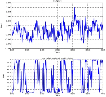
We first present a simulation in the time domain. Figure 1 shows the time pattern of output, stock prices and inflation produced by the model. We observe a strong cyclical movement in the output gap. The source of these cyclical movements is seen to be the weight of optimists and pessimists in the market (see second panel of Figure 1). The model in fact generates endogenous waves of optimism and pessimism. During some periods pessimists dominate and this translates into below average output growth. These pessimistic periods are followed by optimistic ones when optimistic forecasts tend to dominate and the growth rate of output is above average. These waves of optimism and pessimism are essentially unpredictable. Other realisations of the shocks produce different cycles with the same general characteristics.

The third panel of Figure 1 shows the evolution of the stock prices in the time domain. The model creates periods of bullish and bearish behaviour of the stock prices that are associated with the same waves of optimism and pessimism (second panel). The model is also capable of creating what appears to be a bubble and a crash (around period 300). This feature is regularly found in the simulations of the stock prices in the time domain.

pessimistic rule. The ‘contagion-effect’ leads to an increasing use of the optimistic belief to forecast the output-gap, which in turn stimulates aggregate demand and leads to a bull stock market. Optimism is therefore self-fulfilling. A boom is created. At some point, negative stochastic shocks make a dent in the MSFE of the optimistic forecasts. The pessimistic belief becomes attractive and therefore fashionable again. The stock market and the economy turn around.

The last panel of Figure 1 shows the simulated inflation. Inflation is kept within a relatively narrow band around the target (0%) most of the time. Occasionally, it goes beyond this band. This feature is found repeatedly in different simulations of the model. It has to do with the fact that occasionally the extrapolators in forecasting inflation tend to dominate the market. As a result, the credibility of inflation targeting is reduced allowing the inflation rate to drift away from its target. We will come back to this problem and analyse under what conditions the credibility of the inflation targeting regime can be enhanced.

Figure 1. Output gap, inflation and stock prices

100 150 200 250 300 350 400 -0.04

-0.03 -0.02 -0.01 0 0.01 0.02 0.03 0.04 0.05 0.06

Time

Lev

el

output

100 150 200 250 300 350 400

0 0.1 0.2 0.3 0.4 0.5 0.6 0.7 0.8 0.9 1

Time

L

e

v

e

l

100 150 200 250 300 350 400 0.7

0.8 0.9 1 1.1 1.2 1.3 1.4 1.5 1.6 1.7

Time

L

e

ve

l

sha re price s

100 150 200 250 300 350 400

-0.04 -0.03 -0.02 -0.01 0 0.01 0.02 0.03 0.04

Time

L

e

ve

l

infla tion

3.

‘Leaning against the wind’ in the stock markets

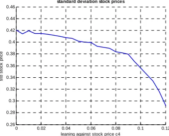
In this section we analyse the issue of the effectiveness of a ‘leaning against the wind’ strategy used by the central bank to limit the fluctuations in the stock prices. We will ask the question of whether this strategy improves the central bank’s capacity of stabilising output and inflation. Thus, we take the view that attempts to reduce stock price fluctuations should be gauged by the success they have in reducing inflation and output volatility.

The way we attempt to answer this question is as follows. We simulated the model under different assumptions about the intensity of the ‘leaning against the wind’ strategy in the stock

market as measured by the coefficient c4 in the Taylor rule equation. We selected values of c4

ranging from 0 to 0.12. For each of these parameter values we simulated the model over 1000 periods and computed the standard deviations of output, inflation and stock prices. We repeated this exercise 100 times and computed the mean standard deviations obtained for each value of

c4. We show the results in Figure 2. We observe the following. As c4 increases the standard

deviations of output, inflation and stock prices decline. At some point, i.e. when c4 comes close

to 0.1 the standard deviations of output and inflation increase dramatically, while the standard deviation of the stock prices declines significantly. Thus, as long as the ‘leaning against the wind’ strategy is moderate, this strategy pays of and reduces the volatility of inflation, output

and stock prices. When this strategy becomes too active (too large a value of c4), it creates

Figure 2. Macroeconomic volatility and ‘leaning against the wind’

0 0.01 0.02 0.03 0.04 0.05 0.06 0.07 0.08 0.09 0.1 0.018

0.019 0.02 0.021 0.022 0.023 0.024 0.025

leaning against stock price c4

s

td out

put

standard deviation output

0 0.01 0.02 0.03 0.04 0.05 0.06 0.07 0.08 0.09 0.1 0.025

0.03 0.035 0.04 0.045 0.05 0.055

leaning against stock price c4

std

p

standard deviation inflation

0 0.02 0.04 0.06 0.08 0.1 0.12 0.26

0.28 0.3 0.32 0.34 0.36 0.38 0.4 0.42 0.44 0.46

leaning against stock price c4

s

td s

toc

k

pr

ic

e

standard deviation stock prices

4.

Inflation targeting and macroeconomic stability

Our previous analysis was conducted in an environment of inflation targeting in which, however, agents maintained their scepticism about the credibility of the inflation targeting regime. As a result, as we have seen, the inflation rate occasionally departs from its target in a substantial way. Thus we modelled a regime of imperfect credibility of the inflation target.

In this section we analyze two extreme cases concerning the credibility of the inflation target. One is to assume that it is 100% credibility; the other assumption is that there is no credibility at all. We take these two extremes, not because these are particularly realistic, but rather to focus on how different degrees of credibility affect macroeconomic stability and the capacity of the monetary authorities to enhance stability by leaning against the wind strategies in the stock markets.

The way we model these two extremes is as follows. In the perfect credibility regime we assume

that all agents perceive the central bank’s announced inflation target

π

They use this value as their forecast of future inflation, i.e. 1 *

~

t t t

E

π

π

The other extreme case, i.e. zero credibility of the inflation target, is modelled symmetrically. Now no agent attaches any credibility to the announced inflation target, and therefore each of

them is an ‘extrapolator’. As before, this is defined by

E

=

π

switching to the alternative forecasting rule.

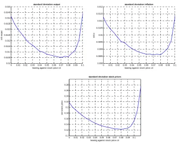
We show the results of these two exercises in figures 3 and 4. Let us concentrate on Figure 3 first, showing the degree of macroeconomic volatility in a regime of 100% credibility of the inflation target. A first thing to note is that in a regime of full credibility of the inflation target the volatility of the output, inflation and stock prices is significantly lower as compared to the regime of imperfectly credible inflation target. The difference is quite high. Comparing Figure 3 with Figure 2 shows that in a fully credible inflation targeting regime the standard deviation of output, inflation and stock prices are about half as large as in the case of imperfect credibility. Thus, credibility is extremely valuable. It allows reducing the volatility of all three macroeconomic variables, at no apparent cost.

A second conclusion from a comparison of Figures 3 and 2 is that mild forms of ‘leaning against the wind’ in the stock market have a much stronger effect in reducing volatility of output, inflation and stock prices. Thus, credibility of the inflation target makes ‘leaning against the wind’ in the stock markets more effective in reducing macroeconomic volatility. (Note again

that this only holds for relatively low levels of c4)

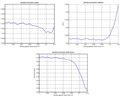
The importance of credibility as a means to achieving macroeconomic stability and as a way to make ‘leaning against the wind’ in the stock market an effective stabilisation tool is reinforced by the results of Figure 4. These show that when there is total absence of credibility in the

inflation target, the volatility of output, inflation and stock prices is higher for all values of c4. In

addition, ‘leaning against the wind’ in the stock market, now has almost no stabilising properties for output and inflation (compare Figure 4 with Figure 2).

Figure 3. Macroeconomic volatility when inflation target is 100% credible

0 0.01 0.02 0.03 0.04 0.05 0.06 0.07 0.08 0.09 0.1 0.01

0.0105 0.011 0.0115 0.012 0.0125 0.013 0.0135 0.014 0.0145 0.015

leaning against stock price c4

s

td o

u

tput

standard deviation output

0 0.01 0.02 0.03 0.04 0.05 0.06 0.07 0.08 0.09 0.1 0.008

0.0085 0.009 0.0095 0.01 0.0105 0.011 0.0115 0.012

leaning against stock price c4

st

d

p

standard deviation inflation

0 0.01 0.02 0.03 0.04 0.05 0.06 0.07 0.08 0.09 0.1 0.1

0.12 0.14 0.16 0.18 0.2 0.22 0.24 0.26 0.28

leaning against stock price c4

s

td s

toc

k

pri

c

e

Figure 4. Macroeconomic volatility when inflation target is 0% credible

0 0.02 0.04 0.06 0.08 0.1 0.12 0.018

0.019 0.02 0.021 0.022 0.023 0.024 0.025

leaning against stock price c4

s

td out

put

standard deviation output

0 0.02 0.04 0.06 0.08 0.1 0.12 0.03

0.035 0.04 0.045 0.05 0.055

leaning against stock price c4

std

p

standard deviation inflation

0 0.02 0.04 0.06 0.08 0.1 0.12 0.26

0.28 0.3 0.32 0.34 0.36 0.38 0.4 0.42 0.44 0.46

leaning against stock price c4

st

d

st

o

ck p

ri

c

e

standard deviation stock prices

5.

The trade-off between output and inflation variability

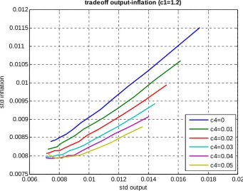
Another way to evaluate ‘leaning against the wind’ strategies in the stock markets is to analyze how they affect the trade-off between output and inflation variability. We will proceed as follows. We return to the regime of imperfectly credible inflation target. We assume several

values of c4 from 0 to 0.05 (the ‘leaning against the wind’ parameter in the stock market). We

then compute the tradeoffs between output and inflation variability in the usual way.8 We plot

the results in Figure 5.

A first important finding concerns the shape of these trade-offs. We find that these trade-offs are non-linear, i.e. there is a positively and a negatively sloped segment. The interpretation is the

following. When the central bank does not care about output stabilisation (c2=0) we are located

in the upper right points of the tradeoffs. An increase in the willingness to stabilise output (c2

increases) leads to a downward movement along the trade-off. This means that when the central bank increases its output stabilisation effort it reduces both the variability of output and

8

That is, we allow the output stabilisation parameter (c2) in the Taylor rule to increase from 0 to 1 and

compute the standard deviations of output and inflation for each value of c2. Note that the output

stabilisation coefficient has much larger values than the stock price coefficient (c4). This has to do with

inflation. At some point, however, applying more stabilisation (c2 increases further) brings us in the upward sloping part. From then on more stabilisation leads to the traditional trade-off: more output stability is bought by more inflation variability. This is the standard result obtained in rational expectations models. In these models any attempt to stabilise output leads to more inflation variability. In our behavioural model this is not necessarily the case. Mild forms of

output stabilisation (low c2) have the effect of reducing both output and inflation variability.

When however the ambition to stabilise output is too strong, we return to the traditional negatively sloped trade-off and the gain in output stabilisation leads to more inflation variability. Thus, in our model some output stabilisation is always better than no stabilisation at all. This result comes from the structure of our model. When the central bank applies modest output stabilisation it also reduces the waves of optimism and pessimism. The latter affect not only output variability but also inflation variability. Thus by reducing these ‘animal spirits’ the central bank achieves both lower output and inflation variability. It can do this because it profits from a credibility bonus. Too much activism, however, destroys this credibility bonus, leading to the normal negatively sloped tradeoffs.

A second finding from Figure 5 relates to the effect of ‘leaning against the wind’ in the stock market. We find that a more intense ‘leaning against the wind’ in the stock market improves the tradeoffs, i.e. shifts them downwards. Thus ‘leaning against the wind’ reduces both output and inflation variability. Note, however, that this result only holds in the positively sloped segment of the tradeoffs. In the negatively sloped part, there is no clear effect of leaning against the wind strategies. This suggests that ‘leaning against the wind’ strategies are effective in reducing both output and inflation variability for the same reason as output stabilisation does. These strategies tend to reduce the scope for waves of optimism and pessimism and thus stabilise the macroeconomy as a whole. A too aggressive use of these strategies, however, will tend to create an inflationary bias, which then re-establishes the negative trade-off between output and inflation variability.

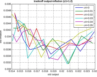
As in the previous section we analyzed the importance of the credibility of inflation. We do this by assuming the same two extreme regimes, perfect credibility and zero credibility. The perfect credibility case is shown in Figure 6. It confirms some of the results obtained earlier. For example, the tradeoffs under perfect credibility are located much lower than those obtained under imperfect credibility (compare Figure 5 with Figure 4). Thus, credibility dramatically improves the tradeoffs, leading to less variability of both output and inflation. We also find that ‘leaning against the wind’ strategies improves these tradeoffs significantly, thus lowering both output and inflation variability.

Figure 5. Trade-off output and inflation variability: Imperfect credibility

0.01 0.012 0.014 0.016 0.018 0.02 0.022 0.024 0.0285

0.029 0.0295 0.03 0.0305 0.031 0.0315

std output

s

td i

n

fl

at

io

n

tradeoff output-inflation (c1=1.2)

c4=0 c4=0.01 c4=0.02 c4=0.03 c4=0.04 c4=0.05

Figure 6. Trade-off output and inflation variability: perfect credibility

0.006 0.008 0.01 0.012 0.014 0.016 0.018 0.02 0.0075

0.008 0.0085 0.009 0.0095 0.01 0.0105 0.011 0.0115 0.012

std output

s

td i

n

fl

at

io

n

tradeoff output-inflation (c1=1.2)

Figure 7. Trade-off output and inflation variability: zero credibility

0.014 0.015 0.016 0.017 0.018 0.019 0.02 0.021 0.022 0.023 0.024 0.033

0.0332 0.0334 0.0336 0.0338 0.034 0.0342 0.0344 0.0346 0.0348 0.035

std output

s

td i

n

fl

at

io

n

tradeoff output-inflation (c1=1.2)

c4=0 c4=0.01 c4=0.02 c4=0.03 c4=0.04 c4=0.05

6. Conclusion

Should central banks use their interest rate instrument to influence the asset prices and to prevent bubbles from emerging? This question has been hotly debated by economists. It has become topical again since the credit crisis erupted in August 2007. We analysed this question using a behavioural macroeconomic model. This model produces booms and busts that arise from the fact that beliefs about the future become correlated. It is the appropriate one to study this question.

17 |

Anderson, S., A. de Palma and J-F Thisse (1992), Discrete Choice Theory of Product

Differentiation, Cambridge, MA: MIT Press.

Azariadis, C. (1981), “Self-Fulfilling Prophecies”, Journal of Economic Theory, 25, 380-96.

Benhabib, Jess and Roger E.A. Farmer (1994), “Indeterminacy and Increasing Returns”,

Journal of Economic Theory, 63: 19-46.

Bernanke, B. and M. Gertler (1995), “Inside the Black Box: The Credit Channel of Monetary

Transmission”, Journal of Economic Perspectives, 9, Fall, pp. 27-48.

Bernanke, B. and M. Gertler (2001), “Should central banks respond to movements in asset

prices?”, American Economic Review, pp. 253-257, May.

Bernanke, B. (2003), “Monetary Policy and the Stock Market”, Public Lecture, London School of Economics, London, 9 October.

Binder, M., and M.H. Pesaran (1996), “Multivariate Rational Expectations Models and Macroeconomic Modelling: A Review and Some Results”, in M.H. Pesaran and M.

Wickens (eds.), Handbook of Applied Econometrics: Macroeconomics.

Bordo, M., and O. Jeanne (2002), “Monetary Policy and Asset Prices”, International Finance,

5, pp. 139-64.

Borio, C. and W. White (2004), Whither monetary and financial stability? The implications of

evolving policy regimes, BIS Working Papers, No. 147, February.

Branch, W. and G. Evans (2006), “Intrinsic heterogeneity in expectation formation”, Journal of

Economic Theory, 127, 264-95.

Brazier, A., R. Harrison, M. King and T. Yates (2006), The danger of inflating expectations of

macroeconomic stability: heuristic switching in an overlapping generations monetary model, Working Paper No. 303, Bank of England, August.

Brock, W. and C. Hommes (1997), “A Rational Route to Randomness”, Econometrica, 65,

1059-1095

Camerer, C., G. Loewenstein and D. Prelec (2005), “Neuroeconomics: How neuroscience can

inform economics”, Journal of Economic Literature, 63(1), 9-64.

Clarida, R., J. Gali and M. Gertler (1999), “The Science of Monetary Policy, A New Keynesian

Perspective”, Journal of Economic Literature, 37, 1661-1707.

Cecchetti, S., H. Genberg, J. Lipsky and S. Wadhwani (2000), “Asset Prices and Central Bank

Policy”, Geneva Reports on the World Economy, vol. 2, Geneva, International Center

for Monetary and Banking Studies, and London, CEPR, July.

Della Vigna, S. (2007), Psychology and Economics: Evidence from the Field, NBER Working

Paper, No. 13420.

Estrella, A. and J. Furher (1998), Dynamic Inconsistencies: Counterfactual Implications of a

Class of Rational Expectations Models”, American Economic Review, 92(4), Sept.,

1013-1028.

Farmer, Roger, E.A. (2006), “Animal Spirits”, Palgrave Dictionary of Economics.

Galí, J. (2008), Monetary Policy, Inflation and the Business Cycle, Princeton, NJ: Princeton

Gigerenzer, G. and P.M. Todd (1999), Simple Heuristics That Make Us Smart, New York, NY: Oxford University Press.

Goodhart, C. and B. Hoffmann (2004), Deflation, credit and asset prices, Financial Market

Group, London School of Economics, Working Paper.

Greenspan, A. (2007), The Age of Turbulence: Adventures in a New World, London: Penguin

Books.

Kahneman, D. and A. Tversky (1973), “Prospect Theory: An analysis of decisions under risk”,

Econometrica, 47, 313-327

Kahneman, D. and A. Tversky (2000), Choices, Values and Frames, New York, NY:

Cambridge University Press.

Kahneman, D. (2002), “Maps of Bounded Rationality: A Perspective on Intuitive Judgment and Choice”, Nobel Prize Lecture, 8 December, Stockholm.

Kahneman, D. and R. Thaler (2006), “Utility Maximization and Experienced Utility”, Journal

of Economic Perspectives, 20, 221-234.

Roubini, N. (2006), “Why central banks should burst bubbles”, mimeo, Stern School of Business, New York University, New York.

Sargent, T. (1993), Bounded Rationality in Macroeconomics. Oxford: Oxford University Press.

Schwartz, A. (2002), Asset Price Inflation and Monetary Policy, NBER Working Paper No.

9321, November.

Sims, C. (2005), Rational Inattention: A Research Agenda, Discussion Paper, no. 34/2005,

Deutsche Bundesbank.

Smets, F. (1997), Financial asset prices and monetary policy: theory and evidence, BIS

Working Papers No. 47, September.

Smets, F. and R. Wouters (2003), “An Estimated Dynamic Stochastic General Equilibrium

Model”, Journal of the European Economic Association, 1, 1123-1175.

Stanovich, K. and R. West (2000), “Individual differences in reasoning: Implications for the

rationality debate”, Behavioural and Brain Sciences, 23, 645-665.

Svensson, L. (1997), “Inflation Forecast Targeting: Implementing and Monitoring Inflation

Targets”, European Economic Review, 41: 111-46.

Tversky, A. and D. Kahneman (1981), “The framing of decisions and the psychology of

choice”, Science, 211, 453-458.

Walsh, C. (2003), Monetary Theory and Policy, Cambridge, MA: MIT Press.

Woodford, M. (2003), Interest and Prices: Foundations of a Theory of Monetary Policy,

19 |

pstar = 0; % the central bank's inflation target

a1 = 0.5; %coefficient of expected output in output equation

a2 = -0.2; %a is the interest elasticity of output demand

a3 = 0.05; %a3 is the elasticity of demand with respect to share prices

b1 = 0.5; %b1 is coefficient of expected inflation in inflation equation

b2 = 0.05; %b2 is coefficient of output in inflation equation

b3 = 0.02; %b3 is the elasticity of supply with respect to share prices

c1 = 1.5; %c1 is coefficient of inflation in Taylor equation

c2 = 0.5; %c2 is coefficient of output in Taylor equation

c3 = 0.5; %interest smoothing parameter in Taylor equation

c4 = 0.0; %stock price smoothing parameter in Taylor equation

β = 0.01; %fixed divergence in beliefs

gamma = 10000; %switching parameter gamma in Brock Hommes

sigma1 = 0.005; %standard deviation shocks output

sigma2 = 0.005; %standard deviation shocks inflation

sigma3 = 0.005; %standard deviation shocks Taylor

rho=0.5; %rho measures the speed of declining weights omega in mean squares

About

CEPS

Place du Congrès 1 • B-1000 Brussels Tel : 32(0)2.229.39.11 • Fax : 32(0)2.219.41.51 E-mail: [email protected]

Website : http://www.ceps.be Bookshop : http://shop.ceps.be Founded in Brussels in 1983, the Centre for

European Policy Studies (CEPS) is among the most experienced and authoritative think tanks operating in the European Union today. CEPS serves as a leading forum for debate on EU affairs, but its most distinguishing feature lies in its strong in-house research capacity, complemented by an extensive network of partner institutes throughout the world.

Goals

• To carry out state-of-the-art policy research leading to solutions to the challenges facing Europe today. • To achieve high standards of academic excellence

and maintain unqualified independence. • To provide a forum for discussion among all

stakeholders in the European policy process. • To build collaborative networks of researchers,

policy-makers and business representatives across the whole of Europe.

• To disseminate our findings and views through a regular flow of publications and public events.

Assets

• Complete independence to set its own research priorities and freedom from any outside influence. • Formation of nine different research networks,

comprising research institutes from throughout Europe and beyond, to complement and

consolidate CEPS research expertise and to greatly extend its outreach.

• An extensive membership base of some 120 Corporate Members and 130 Institutional Members, which provide expertise and practical experience and act as a sounding board for the utility and feasability of CEPS policy proposals.

Programme Structure

CEPS carries out its research via its own in-house research programmes and through collaborative research networks involving the active participation of other highly reputable institutes and specialists.

Research Programmes

Economic & Social Welfare Policies

Energy, Climate Change & Sustainable Development EU Neighbourhood, Foreign & Security Policy Financial Markets & Taxation

Justice & Home Affairs

Politics & European Institutions Regulatory Affairs

Trade, Development & Agricultural Policy

Research Networks/Joint Initiatives

Changing Landscape of Security & Liberty (CHALLENGE) European Capital Markets Institute (ECMI)

European Climate Platform (ECP)

European Credit Research Institute (ECRI)

European Network of Agricultural & Rural Policy Research Institutes (ENARPRI)

European Network for Better Regulation (ENBR)

European Network of Economic Policy Research Institutes (ENEPRI)

European Policy Institutes Network (EPIN) European Security Forum (ESF)