Some problems with seismic reflection techniques

SOME PROBLEMS WITH SEISMIC REFLECTION TECHNIQUES

by

Gregory John Blackburn, B.Sc.(Hons.)

Submitted in partial fulfilment of the requirements for the degree of

Doctor

of, Philosophy.

UNIVERSITY OF TASMANIA

Hobart

1982

, This thesis contains no material which has been accepted for the award of any other degree or diploma in any university, and, to the best of my knowledge and belief, the thesis contains no copy or paraphrase of material previously published or written by another person, except where due

reference is made in the text of the thesis.

CONTENTS

2.1

3.1

4.1

5.1

6.1

R.1

A1.1

A2.1

A3.1

A4.1 Figures

Abstract

Acknowledgements

Chapter CONCLUSIONS

REFERENCES

Appendix 1 RAY TRACING SYSTEM 7 TWO DIMENSIONS

Appendix 2 RAY

TRACING USING FERMAT'S PRINCIPLE

Appendix 3

THOMPSON-HASKELL METHOD

Appendix 4

COMPUTER PROGRAM LISTING (MICROFILM)

Chapter 1 INTRODUCTION

Chapter 2 ERRORS IN VELOCITY CONVERSION FOR SIMPLE GEOLOGICAL STRUCTURES

Chapter 3 STATIC CORRECTION IN IRREGULAR OR STEEPLY DIPPING WATER-BOTTOM ENVIRONMENTS

Chapter 4 SEISMIC VELOCITY AND MIGRATION DETERMINATION

LIST OF FIGURES

Fig. 2.1 Idealised view of a reflection profile.

2.2 Schematic geological section depicting areas for

velocity analysis. 2.6

2.3 _{Schematic geological section showing actual raypaths}

and hypothetical raypaths for a vertical CRP. 2.10 2.4 Schematic geological section containing a high velocity

inhomogeneity. 2.10

2.5 Schematic T 2 -X 2 plots for a reflector whose arrival time due to migration or raypath distortion problems is earlier than for the homogeneous case (A) or where the

arrival time is later than expected (B). 2.11 2.6 Wedge model with corresponding error-factor plot. 2.15 2.7 Unconformity model with corresponding zero-offset

raypaths and error-factor plots. 2.17 2.8 Selected gather locations along the unconformity model

for surface 6 and their corresponding time-difference

plots. 2.18

2.9 Unconformity variation-factor and gather plots at

selected gather locations. 2.19

2.10 Timing and depth errors for the unconformity model. 2.24 2.11 High velocity patch reef model with corresponding

zero-offset raypaths and error-factor plots. 2.25 2.12 Selected gather locations along the reef model for

surface 8. 2.26

2.13 Patch reef time-difference plots for surface 8. 2.26 2.14 Patch reef variation-factor plots. 2.28 2.15 Patch reef variation-factor plots. 2.28 2.16 High velocity fill channel model with corresponding

zero-offset raypaths and error-factor plots. 2.31 2.17 Gathers and time-difference plots for selected

locations along the surface of the high velocity fill

channel model for surface 5. 2.32

2.18 Gathers at E, and time-difference plots for the high

velocity fill channel base. 2.35

2.19 Selected gather locations for the high velocity channel

fill model along surface 8. 2.35

2.20 High velocity fill channel time-difference plots for

surface 8. 2.36

2.21 High velocity fill channel variation-factor plots. 2.36 2.22 Low velocity fill channel model with corresponding

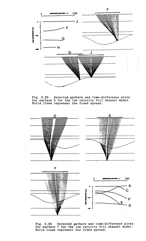
zero-offset raypaths and error-factor plots. 2.38 2.23 Selected gathers and time-difference plots for surface

5 for the low velocity fill channel model. 2.39 2.24 Selected gathers and time-difference plots for surface

7 for the low velocity fill channel model. 2.39

. ii

iii List of Figures cont.

page

Fig. 2.25 Low velocity fill channel model variation-factor and

gather plots at selected gather locations for surface 7. 2.42

2.26 Synclinal model with corresponding zero-offset raypaths

and error-factor plots. 2.43

2.27 Selected gather locations for surface 6 and their corresponding time-difference plots for the synclinal

model. 2.44

2.28 Syncline model variation-factor plots at selected

gather locations. 2.44

2.29 Anticline model with corresponding zero-offset raypaths

and error-factor plots. 2.46

2.30 Selected gather locations for surface 7 for the anticline

model. 2.47

2.31 Selected gather locations for surface 6 and their

corres-ponding time-difference plot for the anticline model. 2.48

2.32 Anticline model variation-factor and gather plots at

selected gather locations. 2.49

2.33 Prograding delta model with corresponding zero-offset

raypaths and error factor plots. 2.51

2.34 Selected gather locations for surface 4 and their corresponding time-difference plots for the prograding

delta model. 2.52

2.35 Selected gather locations for surface 6 and their corresponding time-difference plots for the prograding

delta model. 2.55

2.36 Selected gather locations for surface 10 and their corresponding time-difference plots for the prograding

delta model. 2.56

2.37 Prograding delta model variation-factor curves at

selected gather locations for surface 6. 2.57

2.38 Prograding delta model variation-factor and gather plots

at selected gather locations for surface 10. 2.58

2.39 Timing and depth errors for the prograding delta model. 2.61

3.40 Shelf margin model and corresponding error-factor plot. 2.62

2.41 Seismic stratigraphic interpretation for line 1. 2.66

2.42 Seismic stratigraphic interpretation for line 2. 2.67

2.43 Seismic stratigraphic interpretation for line 6. 2.68

2.44 Seismic stratigraphic interpretation for line 7. 2.69

2.45 Location and depth structure maps for horizons 1 to 7. 2.70

2.46 Synthetic seismogram and velocity and density logs for

drillhole 5. 2.71

2.47 Time-depth curves, interval and average velocity plots

for drillhole 5. 2.72

2.48 Isochrons for the seismic stratigraphic sequences. 2.73

List of Figures cont.

iv

page Fig. 2.50 Interpreted stacking velocities and calculated stacking

velocities for seven horizons on line 6. 2.75 3.1 Earth model illustrating'raypaths to two horizons. 3.4 3.2 The relationships along source coordinate s, geophone

receiver coordinate g, offset coordinate f = g-s, and

mid-point coordinate g = (g+s)/2 (after Claerbout, 1976). 3.4 3.3 Geometry of a wavefront approaching receivers (after

Shah, 1973). 3.8

3.4 Earth model illustrating the shot replacement and

receiver replacement length. 3.8

3.5 Model of a deep water canyon overlying a series of

'horizontal layers. 3.11

3.6 Canyon model gather plots together with wavefront shot

and.geophone statics for three surfaces at four locations. 3.12 3.7 Velocity,profiles for the canyon model. 3.13 3.8 Seismic section together with its corresponding model for

and irregular water-bottom layer overlying a series of

sub-horizontal layers. 3.15

3.9 Velocity profiles for the irregular water-bottom model. 3.16 3.10 Irregular water-bottom model gathered plots together with

wavefront static curves for three surfaces at four

locations. 3.18

4.1 Schematic geological section showing actual raypaths and

hypothetical raypaths for a Vertical CRP. 4.2 4.2 Schematic geological section containing a high velocity

inhomogeneity. , _4.3

4.3 . Plane dipping layer model. 4.5 4.4 Hypothetical curved reflector model. 4.8 4.5 Synthetic CDP gathers and their stacking velocity

distribution. 4.9

4.6 Near, middle and far, traces for the synthetic gathers

generated at location A. 4.10

4.7 Near, middle and far traces for the synthetic gathers

generated at location B. 4.11

4.8 The seismic problem. Given a time trace, can reflection events A, B and C be placed in their correct spatial

position? 4.12

4.9 Three-dimensional plane dipping model. 4.16 4.10 Relationship between the perpendicular to a plane and

the profile line to the dip of the interface (0) and

' the directional angle. 4.17

• 4.11 Ratio of the stacking velocity to the overburden

List of Figures cont.

page Fig. 4.12 Raypath geometry for a diffracting point. 4.22

4.13 , Irregular water bottom layer model and its velocity

profile. 4.25

4.14 Selected traces for the gather at location A. 4.26 4.15 The relationship among source coordinate S, geophone

receiver coordinate g, offset coordinate 1 = g-s,

and midpoint coordinate y = (g+s)/2. 4.28 4.16 ' Geometry of a wavefront approaching receivers. 4.30

waves for three layered media (after Paige, 1973). 5.14 5.10 Amplitude reflectivities for models 1, 3, 4, 6, 7 and 8. 5.18 5.11 Phase reflectivities for models 1, 3, 4, 5, 6, 7 and 8. 5.19

5.19 Amplitude reflectivities for direct and total waves for

varying bed velocity ratios. 5.35

5.19 Amplitude reflectivities for direct and total waves for

varying bed velocity ratios. 5.35 5.20 Typical density ranges for various geological rock types. 5.35

5.21 Velocity-density relationships for common sedimentary rocks (after Gardner et al., 1974)

5.20 Typical density ranges for various geological rock types. 5.35

5.21 Velocity-density relationships for common sedimentary

rocks (after Gardner et al., 1974) 5.36

omain due to two reflectors having the same polarity and opposite

polarity. 5.6

5.4 Sequence composed of a number of thin layers. 5.6 5.5 Typical synthetic seismogram exhibiting no interference

effects (after Dunkin & Levin, 1973). 5.10

5.6 NMO corrected gather. 5.11

5.7 Raypath geometries for a thin layer. 5.13 5.8 Models of thinly laminated media and their corres-

ponding layer parameters. 5.13

5.9 Reflection coefficients for direct normal incidence

5.12 Amplitude variations for both the total and direct

waves for models 1, 4, 7 and 8. 5.21 5.13 Intrabed multiple raypaths. 5.21 5.14 Frequency-thickness amplitude reflectivity variations

for various incident angles - model 1. 5.25

5.15 Frequency-thickness phase reflectivity variations for an

incident angle of 1 degree - model 1. 5.27

5.16 Zero-phase and non-zero-phase wavelets (after Anstey,

1977). 5.30

5.17 Compressional velocity ranges for various geological

rock types. 5.32

5.18 Amplitude and phase reflectivities for varying bed

velocities. 5.33'

List of Figures cont.

Fig. 4.15 Ricker wavelet with a dominant frequency of 30 hZ and its frequency spectrum.

4.16 High velocity channel fill together with stacking and rms velocity curves and stacked sections for surface 8.

4.17 Selected gather locations for the high velocity channel fill model and their corresponding relative amplitudes for horizon 8.

page 4.20 4.22 4.23 5.4 5.5 4.23 5.4 5.5 on of the frequency content of the far trace

wavelets due to NMO correction of a CDP gather. 5.2 Uncorrected CDP gather illustrating that amplitude

variations are frequency as well as offset dependent. 5.3 Interference effects in frequency domain due to two

reflectors having the same polarity and opposite

polarity. 5.6

5.4 Sequence composed of a number of thin layers. 5.6 5.5 Typical synthetic seismogram exhibiting no interference

effects (after Dunkin & Levin, 1973). 5.10

5.6 NMO corrected gather. 5.11

5.7 Raypath geometries for a thin layer. 5.13 5.8 Models of thinly laminated media and their corres-

ponding layer parameters. 5.13

5.9 Reflection coefficients for direct normal incidence

waves for three layered media (after Paige, 1973). 5.14

5.12 Amplitude variations for both the total and direct

waves for models 1, 4, 7 and 8. 5.21 5.13 Intrabed multiple raypaths. 5.21 5.14 Frequency-thickness amplitude reflectivity variations

for various incident angles - model 1. 5.25 5.15 Frequency-thickness phase reflectivity variations for an

incident angle of 1 degree - model 1. 5.27 5.16 Zero-phase and non-zero-phase wavelets (after Anstey,

1977). 5.30

5.17 Compressional velocity ranges for various geological

rock types. 5.32

5.18 Amplitude and phase reflectivities for varying bed

velocities. 5.33

5.19 Amplitude reflectivities for direct and total waves for

varying bed velocity ratios. 5.35

5.20 Typical density ranges for various geological rock types. 5.35 5.21 Velocity-density relationships for common sedimentary

vi

List of Figures cont.

page

Fig. 5.22 Amplitude reflectivities for varying density contrasts

for models 1, 4, 7 and 8. 5.38

5.23 Phase reflectivities for varyind density contrasts

for models 1, 4, 7 and 8. 5.39

5.24 Amplitude variations for both the total and direct waves due to varying bed density ratios for models 1,

4, 7 and 8. 5.41

5.25 Amplitude variations for both the total and direct waves due to varying bed density ratios for models 1,

4, 7 and 8. 5.41

5.26 Amplitude and phase reflectivities for various thickness-bed velocity combinations using the model 1 type

parameters. 5.42

5.27 Comparison of conventional and broadband seismic data. 5.44

5.28 Phase spectrum for model 1. 5.46

5.29 Synthetic seismograms for various phase shifted pulses. 5.47

5.30 Coherence measurements used in NMO velocity

determination. 5.51

5.31 Cyclic buildup due to reflection from a single

interface. 5•54

5.32 Onset time variations due to absorption (after Anstey,

1977). 5.54

5.33 Reflection process for two interfaces illustrating

their interference effect. 5.55

5.34 Synthetic seismogram showing complex interference effects

and consequent onset time delay problems. 5.56

5.35 Time pulses for various incident angles showing the difficulties in trace correlation due to amplitude

and phase variations. 5.56

5.36 Intrabed and interbed multiples. 5.58

5.37 Log characteristics of a braided stream sequence. 5.59

5.38 Log characteristics of a beach-shoreface sequence. 5.59

5.39 Braided stream and beach-shoreface models. 5.60

5.40 Amplitude and phase spectra for the braided stream

and shoreface models. 5.61

5.41 Acoustic properties of the brine, oil and gas models. 5.64

5.42 Amplitude reflectivities for PP waves due to brine, oil

and gas saturated sands of varying thickness. 5.65

5.43 Phase reflectivities for PP waves due to brine, oil

and gas saturated sands of varying thicknesses. 5.66

5.44 Comparison of wave trace shapes for the oil, gas and

brine saturated sand models at different incident angles. 5.67

5.45 Comparison of wave trace shapes for oil and gas saturated

sands of varying thicknesses. 5.69

5.46 Time traces for Ricker wavelets having dominant

frequencies of 20, 40, 60, 80 and 100 hz and thicknesses

vi i

List of Figures cont.

page Fig. 5.47 Frequency thickness amplitude and phase reflectivity

variations for normally incident plane waves. 5.71

5.48 Time traces for Ricker wavelets having dominant

frequencies of 20, 40, 60, 80 and 100 hz and velocity contrasts of 0.8, 1.0 and 1.2 (corresponds to bed

velocities of 2536, 3170 and 3804 m/sec). 5.73

5.49 Normal incident amplitude and,phase reflectivities

for varying velocity contrasts. 5.74

5.50 Amplitude reflectivities for mode-converted PS waves

due to brine, oil and gas saturated sands of varying

thicknesses. 5.75

5.51 Phase reflectivities for mode-converted PS waves due

to brine, oil and gas saturated sands of varying

thicknesses. , 5.76

5.52 Four density and somic logs over a 120 m interval

representing varying gross oil columns and their' incident angle dependent amplitude reflectivity

spectra. 5.78

5.53 Density and velocity models for 120 m intervals and

their acoustic impedance logs. ' 5.79

5.54 Normal incident reflectivities for models 1 to 4. 5.80

5.55 Fourier frequency components at 5 hz intervals for

the model 1 shaped spectrum using the approximate

minimum phase (A) and zero-phase (B) spectra. 5.82

5.56 Cepstra (a) and complex cepstra (b) for models 1 to 4. 5.84

5.57 Comparison of the complex cepstrum and impedance log

for model 3. 5.85

5.58 Reflection and refraction of an incident' plane

'compressional wave at a boundary. 5. 91

5.59 PS:PP amplitude ratios for models 1, 4, 7 and 8. 5. 93

5.60 Transmissivity for models 1, 4, 7 and 8. 5. 914

A2.1 Two-dimensional geological model with curved boundaries. A2.2

A2.2 Flow diagram for computer program FERMAT. A2.8

A2.3 Flow diagram for function routine SIMUL. A2.9

A2.4 Three-dimensional geological model with curved boundaries. A2.10

ix

ABSTRACT

Non-zero offset raypath tracing of primary P waves over a suite of geologically complex two-dimensional models illustrates that large errors occur in the conversion of stacking velocities to vertical velocities. Consequently (1) stacking velocities

may not be consistent for seismic lines shot over the same

area for different field configurations, (2) stacking velocities can vary greatly for a given spread length and different shot offsets, (3) rapid lateral changes in stacking velocities due to geological factors may disguise velocity information from

horizons overlain by irregularities, (4) the customary assumption that stacking velocities approximate root mean square velocities is not valid in areas of geological complexity, (5) fictitious time shifts and consequent timing and velocity errors are

introduced when conventional replacement statics are used, and (6) statics are time variant and surface inconsistent so that appropriate corrections should be made according to layer depth.

'Simple mathematical expressions are derived for velocity and depth migration determination in both steeply dipping and

'c omplicated overburden environments.

Model studies show that the amplitude, frequency and

wavelet characteristics of a reflector are dependent on both the reflector and overlying formations and may preclude definition of the reflecting surface. The use of CDP methods is detrimental in preserving these essential parameters. Interference due to thin layers results in reflectivities, transmissivities and

ACKNOWLEDGEMENTS

The project was supervised by Dr. John E. Shirley and Dr. Roger J. G. Lewis to whom I am indebted for guidance and assistance. I would also like to thank John and his wife, Jill, for their friendship and hospitality. Discussions with Dr. W. D. Parkinson, Dr. D. E. Leaman and Mr. K. Spence have proved a source of inspiration. I am deeply indebted to Mr. E. Stanford, Geophysical Manager of Esso Australia Ltd.,

who released velocity data, seismic sections and well information over one of their prospects. West Australian Petroleum Pty. Ltd. are also thanked for providing seismic sections.

To Dr. R. G. Richardson for his discussions, inspiration and friendship, and to Ms. J. Pongratz for her thesis production assistance I express my deepest and most sincere thanks.

The study was financed by a University of Tasmania Post-graduate Research Award.

Chapter 1

INTRODUCTION

page

I. INTRODUCTION 1 . 1

1.1

I. INTRODUCTION

This investigation of seismic wavepropagation through geologically complex regions began at a time when CDP based wave equation migration was gaining popularity amongst

exploration geophysicists and problems with migration in complex regions were becoming apparent. Migrated reflection events which appeared On a seismic section rarely corresponded to their true position in space. In areas of moderate dip

(up to 10 0 ) the seismic section approximated the structure with sufficient accuracy to be acceptable. For example the

distortion of anticlinal limbs in simply7fOlded sections was acceptable because the important crestal positions are

horizontal and were thus correctly, positioned.

Coherent seismic events could be transformed to approx-imate the true section by manual migration techniques such as using raypath charts .(Dobrin, 1976, p.240) or by collapsing diffraction curves (Ragedoorn, 1954). Rapid advancement in migration techniques beganwith the introduction of solutions to thewaVe equation to implement the migration process.

Claerbout, An a series of papers (Claerbout, 1970, 1971;

Claerbout & Johnson, 1971; Claerbout & Doherty, 1972), outlined a procedure for propagating a wave field Using finite

1.2

Velocity information in an undrilled region is determined from stacking velocities or by inversion techniques (e.g.Seislog). Dix (1955) developed graphical techniques for determining inter-val and rms velocities. The process has since been automated by performing hyperbolic searches for the maximum semblance of

coherent events for CDP gathered traces (Taner & Koehler, 1969). When used to convert the time section to a depth

section these resulting stacking velocities yield depths which are too large. Al-Chalabi (1973) found that stacking

velocities were accurate to better than 1 percent when the spread length/depth ratio did not exceed unity. He also

noted (Al-Chalabi, 1074) that the difference between stacking velocities and rms velocities increased with increasing

offset.

II. AIMS

Determination of a true depth picture and implementation of the wave equation migration procedure requires an accurate knowledge of the velocity variations within the earth. Thus this thesis was directed at the crucial velocity determination procedures and consideration of the implications of any

deviations from accepted theory. The aims of this thesis are:

(i) to study the effect of non-horizontal anisotropic

velocity layering on the conversion of stacking velocities to vertical velocities by ray tracing;

1 . 3

(iii) to investigate alternatives to the conventional replacement statics techniques. These techniques introduce possible time shifts, timing and velocity errors for long spreads or in regions of irregular near surface geology. Residual statics may also be time variant and surface inconsistent;

(iv) to use modelling techniques to determine the dependence of the amplitude, frequency and wavelet characteristics of an arrival on the section complexities and geological conditions at the reflector;

(v) to study the nature of reflections from thin layers and develop possible techniques for the extraction of the characteristics of these layers from the time traces; and

(vi) to derive mathematical expressions for calculating

velocity distributions and for performing depth migration in complex geological situations.

Initially it was hoped to apply some of the techniques developed to conventional field data but approaches to the

Australian companies or subsidiaries of Broken Hill Proprietary Co. Ltd., Delhi International Oil Corporation, Esso Australia Ltd., Shell Development Pty. Ltd., Utah Development Company, West, Australian Petroleum Pty. Limited, and Woodside

Petroleum Development Pty. Ltd. to obtain CDP gathered field , tapes were unsuccessful. However field situations on sections

supplied by Esso Australia Ltd. and West Australian Petroleum

Chapter 2

ERRORS IN VELOCITY CONVERSION FOR SIMPLE GEOLOGICAL STRUCTURES

I.

II.

III.

IV.

INTRODUCTION

SPREAD DESIGN PHILOSOPHY

VELOCITY MEASUREMENTS AND SOME GEOLOGICAL

CONSTRAINTS

GEOLOGICAL MODELS AND VELOCITY DETERMINATIONS

page

2.1

2.5

2.7

2.8

1. Stratigraphic Wedge 2.14

2. Unconformity 2.16

3. Patch Reef 2.23

4. Buried Channels 2.30

(a) High velocity channel fill 2.30

(b) Low velocity channel fill 2.37

5. Syncline 2.40

6. Anticline 2.45

7. Prograding Delta 2.50

8. Shelf Margin 2.59

V. MIGRATION VELOCITY ESTIMATES 2.59

VI. STACKING VELOCITIES DETERMINED FROM THREE- 2.60

DIMENSIONAL MODELS

2.1

I.

INTRODUCTION

Interpretation of seismic reflections and their

conversion to depth remains a key problem in seismic explor-ation - especially in geologically complex areas. The

difficulty of correctly interpreting geological structures on time sections was illustrated by May & Hron (1978).

Existing velocity estimation techniques based on layered media assumptions (Schneider & Backus, 1968; Taner & Koehler, 1969) are downgraded as the reflectors become curved or discontinuous (Taner et at., 1970; Miller, 1974).

The need for accurate velocity information and discrim-ination between primary and multiple reflections has prompted the use of the common depth point (CDP) method, often

with large shot-geophone offsets. Large offsets result in improved accuracy in the normal moveout (NMO) corrections, due to the large moveout, with resultant improved velocity deter-mination.

Levin (1971) showed that the NMO velocity obtained for a dipping interface overlain by a uniform medium, is always greater than the true medium velocity and is

V

V is the true velocity.

For layered models with reflectors of arbitrary dip and curvature equation (1) often provides the only correction

2.2

In the presence of near-surface anomalies or where lateral velocity anomalies at depth have dimensions of the order of a CDP gather, large errors may occur in moveout based velocity estimates. As the spread is moved across such an anomaly differential traveltime variations are introduced at varying offsets within the CDP set, producing residual moveout errors.

Stacking velocities derived from the NMO correction of CDP gathers need have no physical relationship to

the true velocity distribution below the gather location. They are merely a variable defining the hyperbola which best fits the reflection alignment. For uniform horizontal layers and small offsets the stacking velocity approximates the rms velocity (Dix, 1955).

Shah & Levin (1973) examined the nature of the time-distance curves and velocities determined for models with sub-surface beds separated by plane-horizontal interfaces and noted that the NMO velocity increased monotonically as the spread length increased.

The arrival time (T_x) for various offsets (X) can be given by an infinite series of the form

Tx 2 = C1 C2X2

COO COO

(Taner & Koehler, 1969)

where the coefficients CI, C2, C3, depend on layer thicknesses and interval velocities.

2.3

velocity techniques are based on this truncation. The

stacking velocity equals the rms velocity only where the earth is homogeneous and the higher order terms in the series are zero. Shah & Levin (1973) and Al-Chalabi (1973, 1974) studied the effect on moveout velocities if further terms

are included in the expansion. _{Shah & Levin generated}

horizontally layered sub-surfaces and noted that errors were less than 2 percent when a three-term expansion for T x 2 was used.

After studying over 1000 model cases with randomly generated velocities, Al-Chalabi (1973) found that when the spread length/depth ratio did not exceed unity all results were accurate to better than 0.5 percent. When the spread length/depth ratio increased to two none of the two-term truncation results were accurate to better than 3 percent. Al-Chalabi also showed that in 97 percent of these

cases, a three-term truncation was sufficient to improve the accuracy to better than 1 percent.

Al-Chalabi (1974) noted that the difference between the stacking velocity and rms velocity increased with increasing offset and decreased with increasing depth.

Levin (1979) noted that the P wave moveout velocity found from surface seismic data can deviate from the vertical P wave velocity to a value approaching the horizontal P wave velocity, the actual value depending on the elastic parameters and the spread length used for velocity determination. Levin studied wave propagation in transversely isotropic solids and

2.4

1) as long as the amount of anisotropy is less than 15

percent T 2 -X 2 plots are straight lines that yield moveout velocities lying between the velocities for primary (P) wave travel in the horizontal and vertical directions;

2) for small anisotropy and short spreads the P wave velocity found from a T 2 -X 2 plot is the P wave velocity in the

vertical direction; and

3) for large P wave anisotropy and greatly different values for Poisson's ratio, T 2 -X 2 data do not define a straight line.

In complex areas migration techniques have been used to take into account the deviation in raypaths (Gardner et al., 1974; Schneider, 1971; French, 1974). Velocity interpretation based on migrated data (Claerbout & Doherty, 1972; Sattlegger & Stiller, 1974; Schultz & Claerbout, 1978) has also helped reduce complications. In addition, Doherty & Claerbout (1976) showed that when data is migrated prior to velocity analysis, reflectors of arbitrary curvature can be treated as horizontal layers in velocity estimation procedures. They used finite difference approximations to the wave equation to derive a structure-independent velocity estimator for such models.

The difficulties of correctly interpreting geological

structures on time sections (May & Hron, 1978) and the potential errors in existing velocity techniques for curved or discontin-uous reflectors (Miller, 1974) illustrate that problems may

occur in complex geological areas. Consequently an analysis has been made of the precise contribution of these features on

2.5

I . SPREAD DESIGN PHILOSOPHY

The following requirements need to be satisfied in designing the field layout for CDP data collection: 1) attenuate multiples,

2) improve the signal-to-noise ratio, 3) avoid strong coherent noise,

4) retain vital shallow reflections, and 5) obtain reliable velocity information.

The seismic system is limited by the dynamic range of the recording instruments and consequently the overall requirement is to record target reflections, however contaminated, within this range.

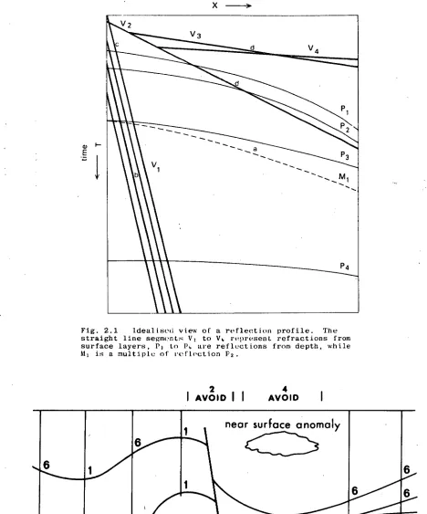
Figure 2.1 represents an idealised reflection profile. 'The straight line segments VI to Vy correspond to refractions

from surface layers. P I to Py are reflections from depth while M I ,is a multiple of the reflection P2.

Attenuation of multiple reflections is accomplished by the use of long spreads so that there is a large difference in residual moveout between the multiple and primary events (a on Figure 2.1). Strong'coherent noise can be avoided by an appropriate choice of offset (b on Figure 2.1). This will indirectly improve the noise ratio. The signal-to-noise ratio can also be increased by increasing the CDP fold. To record the shallow reflections it is imperative that the offset between the shot and nearest geophone be small (c in Figure 2.1). It must be noted that at early times stretching distortions due to NMO correction may be such that only a few traces may be stacked.

shot-receiver distance X --->

Fig. 2.1 Idealised view of a reflection profile. The straight line segments VI to Vy represent refractions from surface layers. PI to Py are reflections from depth, while MI is a multiple of reflection P2.

2 „ 4

I AVOID I I AVOID I

2.7

areas and at long distances strong, straight line. coherent noise occurs (d on Figure 2.1) so that the outer traces may have to be muted.

III. VELOCITY MEASUREMENTS AND SOME GEOLOGICAL CONSTRAINTS

If stacking velocities are to approximate rms velocities / very careful selection of the velocity gather location is

required. Hence -

1) Analyses are positioned at the crests and troughs of folds where conditions approximate uniform horizontal layering

(1 on Figure 2.2). Velocity determinations on the flanks (6 on Figure 2.2) yield velocity distributions which are unrealistically high (Levin, 1971);

2) Gather locations at levels where raypaths have passed through faulted or otherwise disturbed zones (area 2 on 'Figure 2.2) are to be avoided. Within this constraint an

analysis each side of the fault should be made;

3) Analysis at levels where there is obvious interference, for example pinchouts (area 3 on Figure 2.2), is to be avoided; 4) Locations where raypaths pass through an obvious

near-surface anomaly (area 4 on Figure 2.2) should also be avoided; 5) Velocity determinations over areas where fragmentary

reflections are visible at depth (5 on Figure 2.2) may have to be used if they provide the only velocity information at depth; and

6) Other locations should be selected with discretion.

The determination of velocity is critically sensitive to overburden complications. The following points (Anstey, 1977), are generally considered to be true:

a) a local velocity anomaly results in a

static variation in

2.8 b) the largest variations of stacking velocity occur in zones below the ends of anomalies,

C) the variations grow in magnitude and horizontal extent with depth below the anomaly s ,

d) if dip develops at depth, without lateral change of interval velocity in any layer, then the "depth point" for the far traces of the gather move up dip, the NMO

(AT) decreases accordingly and the stacking velocity increases from its "correct" value,

e) if there is no dip, but a smooth lateral change of

interval velocity in any layer, the far trace "depth point" on deeper layers moves in the direction' of the lower velocity, AT decreases and the stacking velocity increases from its

"correct" value,

f) in the general case involving both dip and lateral velocity change, the final effect on stacking velocities is an amalgam of both effects, and

g) whenever a more abrupt change of interval velocity occurs very large swings of stacking velocity occur.

IV.

GEOLOGICAL MODELS AND VELOCITY DETERMINATIONS

The author has developed a two-dimensional ray tracing program (Appendix 1) that allows curved reflectors and lateral velocity variations. Using this program model studies have outlined variations in stacking velocity due to geological structure and spread configuration. Two potential geological causes for velocity variations are defined:

2.9 For the purposes of this thesis this is called the

migration problem.. _{Consider the case where the zero offset}

'ray arrives earlier than the true vertical ray. All the non-zero offset rays will arrive earlier than those for the common reflection point (CRP) below the gather. Hence the stacking velocity as determined from a T 2 -X 2 graph (taken as the square root of the reciprocal of the slope Of a least squares straight line through points on the graph) will be greater than that for the case of a CRP below the gather (Figure 2.3).

2. Errors in stacking velocity due to static variations as a result of overburden complications.

Consider the case (B) shown in Figure 2.4. The outer . traces pass through a lateral inhomogeneity, with higher velocity than the surrounding material. The time of arrival of the far traces is relatively early, so that the least squares best fit line differs from that for the homogeneous case [case (A)]. Thus in this situation the stacking velocity is larger than for the homogeneous case. This is called

the raypath distortion

Offset and spread length induced velocity variations result from migration and raypath distortion problems.

Consider the case where raypath distortions produce earlier arrival times for the far traces than'would be expected for a horizontal layered-casejcase (A) in Figure 2.5]. For the situation in which short and long spreads have the same

shot-first receiver offset it is noted that the stacking

1 / VRMS 2

x

\ 1 / VSTACK 2

TO2

X TVERT 2

1/V RMS 2

T 2

VSTAC K 2

x

2

Fig. 2.3 Schematic geological section showing actual raypaths lines) and hypothetical raypaths for a vertical Cltl , (dashed lines). Corresponding T 2 - -2 A plots show that the zero-offset time is less than the vertical traveltime while actual stackir.g velocities are greater than the root mean square velocities for that location. This is

the migration problem.

A

x

2

sk/Pe = livnmo )A

//'

siope=(I/V_t?rns)

,/''/' ,/'

27r

slope

•

spread A

spread B

reflector

2

X

2.12 arelater than expected [case (B) in Figure 2.5] the stacking velocity for the short spread will be greater than that for the longer spread.

Simplified models of typical geological situations are illustrated in this section. Each gather consists of 72 traces with a geophone separation of 46 m and a shot-first receiver

offset of 46 m. The rays have been traced to within 1 m of the shot and receiver locations. The effect of geological

structure on stacking velocities has been determined using a fixed gather consisting of 24 traces with a shot-first receiver offset of 92 m and a spread length of 2195 m. To emphasize the variations in stacking velocity an error factor approach has been used where the factor is defined as the difference between the stacking velocity derived from ray modelling and the average velocity at the gather location divided by the stacking velocity. The.error factor is expressed as a percentage.

Two arbitrary spreads have been chosen to study the effect of spread length and offset on stacking velocity for the geological models.

The first consists of 24 traces, each having a geophone separation of 46 m. The shot-first receiver offset increases from 46 m to 1104 m in 46 m increments. The second spread consists of 48 traces (36 traces for some models) having the same receiver separation and offset variations as the first case. For convenience these are called short and long spreads. Stacking velocities for each of these spreads and for the range of offsets have been determined. In order to normalise the variation of stacking velocities with offset a variation factor is defined as the ratio of the

2.13 derived from ray modelling and the rms velocity to the rms

velocity, expressed as a percentage. Changes in the variation factor with offset or spread size will thus highlight areas 'exhibiting offset induced velocity problems.

It is necessary to determine what causes the velocity variations. For:uniform-horizontal layers and small offsets the stacking velocity approximates the rms velocity. Thus an excellent gauge can be formed by calculating the difference between the traveltime of the ray traced to a geophone and

the-traveltime calculated from

X 2

+T 2 ...(3)

V 2 _rms. vert

where )Lis the shot to geophone distance

. 1/ is the rms velocity-

rms

T _t is the vertical traveltime. ver

Migration type problems are manifest as time differences for zero offset (X = 0) while departures in time from this zero offset time difference result from raypath distortion. Diagrams based on these factors will be called time difference plots A negative time difference on these plots indicates that the traced ray arrives earlier than the ray calculated using the rMs-velocity and vertical traveltime.

Migration problems are evident when large variation

factors (and hence large:deViations of the stacking velocities from - rms-velocities)'occur for very small offsets, in

particular for the small: spread. Largechanges in the

2.14 affect the accuracy of stacking velocity determination; espec-ially when the geology is not composed of horizontal layers.

In the models, variation factors for both spreads have been plotted as a function of the shot-first receiver offset. Positive variation functions correspond to a stacking velocity, determined by ray tracing, greater than the rms velocity at the particular gather location. The value of the variation factor for a particular offset and spread shows the percentage error of the velocity determination for that location, while differences in the variation factors for the two spreads at the same offset highlight the effect of different spread

lengths on velocity accuracy. An increasing variation-factor value with increasing offset implies a progressively increasing stacking velocity. The converse is also true.

1. STRATIGRAPHIC WEDGE

Figure 2.6 shows a sandstone wedge (P velocity 4270 m/sec) surrounded by a lower velocity shale (3350 m/sec) and the

corresponding error factors for surfaces 5 and 6. Surface 5 can be divided into two distinct regions corresponding to the break in slope at the wedge apex. Applying equation (1) for surface 5 to the right of the wedge and assuming the region above the surface to be homogeneous so that surface 5 may be treated as a single dipping reflector, yields an

2290 ₂ 22aa 3050

3050

3 3350

3350 ₄

4270

3350

4270 5

6

3350

SIOPHONE LOCATION, 2190

A

A

-30 0

4270

0

A BC

0 DISTANCE , metres

11580

ERROR FAC

TOR (

%) _{1 —}

5

3

6

2.16 homogeneous there is an overall increase in the actual

error factors.

Similarly, for surface 6, the apparent error factor is 1.20 percent. As there are no dip breaks along this surface the actual error factor curve tends to be level about a

slightly higher base, with an anomalous zone around the wedge apex. CDP gathers and time difference plots for gathers at locations A (4880 m), B (5790 m) and C (6710 m) show an overall migration time lag of -15 milliseconds. Time

difference plots for the gather at B show a time difference increasing with offset, corresponding to the far traces arriving earlier than would be expected in a horizontally layered situation. This is clearly seen for the gather plot where the far traces travel through a larger portion of the higher velocity wedge material and results in a somewhat

larger stacking velocity and hence larger error factor. The gather at A, on the other hand, shows little time difference between near and far traces relative to the horizontal layered model. The gathered plot indicates that the time spent in the high velocity wedge by the far traces corresponds to that for the near traces. The gather at C is unaffected by the wedge.

2. UNCONFCRMITY

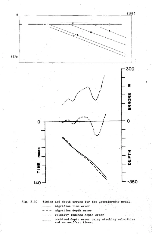
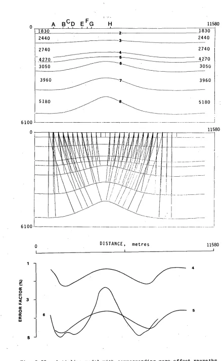
Figure 2.7 shows a simple unconformity. Error-factor plots for surfaces 5, 6 and 7 indicate that severe velocity problems occur for surfaces below the termination of a layer along the unconformity. The effect becomes greater for

deeper surfaces. Time-difference plots (Figure 2.8) for

A

B C E F GH I J

3510 3350 3050 2740

11580

1830 2440

2740

3350

3510 0

1830

2440

4270

3

111'11

111L1 A

11

1L1 i

1111■WAII 11/111/11111111/11M11/ IMII MII

1

0 11580

4880

DISTANCE, metres

11580 1

Fig. 2.7 Unconformity model with corresponding zero-offset raypaths and

71:

1111111

■

tfik

.

-40

5

W-80

P

0 1320INIONE LOCATION; m ₂₁₉₀

A

-120 - AA,,Y

Fig. 2.8 Selected gather locations along the unconformity model for surface 6 and their corresponding

Mgr"

/

N

X _{— 9140 K} 9140K

6400 F

7320 G 7320.G 6400F

5490 D

7

6

VARI

ATION FACTO

R,

X

4 5

3

5490 D

8230

8230

2

7 7

0 1100

1

OFFSET, metres

2.20 A (3350 m) to K (9140 m) the effect of time errors due to

migration, as determined from zero-offset raypath plots, increases. They account for a 40 msec error in timing at B (4270 m) and a 110 msec error at I (7920 m). Superimposed on these errors are• raypath distortions for the non-zero offset rays. The far traces for the gather at location A, for example, arrive later than would normally be expected with a consequent increase in stacking velocity and a smaller •

error factor for that gather. This is because the common reflector point has moved up dip, extending the path of the .far traces in the material above the unconformity. The converse is true at C (4880 m) where the far traces arrive earlier than would normally be expected due to the larger path length for these traces in the high velocity dipping layer between surfaces 5 and 6. However, at location D

(5490 m) the influence of the lower velocity layer between surfaces 4 and 5 retards the middle and far traces

thereby decreasing the error factor. The effect of this low velocity wedge diminishes as the gather location is

moved towards location F (7010 m). The far traces still arrive earlier than would normally be expected thereby

retaining high error factors. Gathers at G (7320 m),

H(7620 m) and I (7920 m) are affected by the additional low velocity wedge material between surfaces 3 and 4 which results in later arrival times as the traces cross over the wedge. Conversion to depth in such areas would be extremely difficult due to the large error in timing because of migration and the subsequent difficulty in conversion to true vertical velocities.

2.21. the long spread has been reduced to 36 traces, partly corres-ponding to the far trace muting routinely applied in

processing shallow reflections. The long spread has a shot-first receiver offset of 92 m and corresponds to the fixed spread configuration. Thus the variation factor values at each location should reflect the general trend of the error factor curve for the fixed spread. The difference in the numerical value results from the differing definitions of the two factors. Migration errors increase from locations A to K. This accounts for the progressively larger stacking velocities relative to the rms velocities and hence the increased positive variation factors with increasing

horizontal distance. Inaccuracies in velocity conversion of up to 7 percent may result. Deviations from this

general-isation are produced by the interplay of raypath distortion and migration problems.

The variation factors for the gather at D exhibit a 1 percent variation in velocity due to different spread lengths and the factors progressively increase with offset (1.5 percent change). This large variation is due mainly to the raypath distortions (Figure 2.9) associated with the wedge-shaped lower velocity layer between surfaces 4 and 5. The effect of this wedge diminishes for the gather at F and there is only a very slight increase of stacking velocities with offset distance. The 4.5 percent error derives mainly from migration errors. Due to the small raypath distortions variation factors for both long and short spreads are similar

(Figure 2.9).

2.22 decreasing stacking velocity. For small offsets the variation factor is constant but as the offset increases beyond 368 m it decreases due to the later arrival of the far traces through the low velocity wedge between surfaces 3 and 4. This delay, combined with the early arrival of the zero-offset time

relative to the true vertical time, results in the

7 percent inaccuracy in velocity conversion. For the larger spread there is a more gradual decrease in the variation factor due to the smearing effect of the increased CDP fold.

The progressive decrease in stacking velocity with offset is pronounced for the gather at J where there is a 3 percent decrease in the variation factor due to offset changes for the short spread. This decrease results from the influence of the lower velocity wedge material between surfaces 3 and 4. The relatively early arrival of the far traces, where one leg of the path does not pass through this wedge material, accounts for the progressive increase in stacking velocity for large offsets. The 2 percent difference in velocities for small offsets indicates potential problems in the choice of spread length sizes over such geological situations.

The raypaths for the gather at K are not influenced by terminating wedges so that raypath distortions are minimal and errors result mainly from migration problems. Thus stacking velocities determined for both spreads and for all offsets are similar. However velocity conversion errors are still large

(5.5 percent).

2.23 (Figure 2.10). These errors when translated into depth values• using true vertical velocities result in underestimates of between 90 and 340 m. Similarly, depths are overestimated by 90 to 260 m when calculated using measured stacking velocities and true vertical times. The partial cancellation of the velocity and timing errors in this particular model reduces the error in depth estimates to a range of only 130 m. The maximum errors occur for gathers above the termination of dipping beds along the unconformity surface.

3. PATCH REEF

Figure 2.11 is an illustration of a high velocity reef model but it could also represent an inhomogeneity in the section. Zero-offset raypaths are also shown. The gathers at A (2440 m) and C (2740 m) receive rays from two locations on surface 5, resulting in two potential stacking velocities. Fixed spread error factors (Figure 2.11) for horizons below surface 5 show large oscillations and stacking velocities less than the true vertical velocities may be obtained.

4270

0 11580

Fig. 2.10 Timing and depth errors for the unconformity model. migration time error

migration depth error

velocity induced depth error

—L11_411

1\ ‘:. -•

• I

i L : ! _

i I i ' • _{1 I}

I 1 '11; I •

, _L

0

:6100

BD EF AC G H I

till I I I

• 11580

1830

2-

3

1830

2440

2740

.3050

5180

3660

4270 2440

2740

4

3050

--

---5 4570

5180 6

3660

7

6100 --- — -

11580

DISTANCE, metres ₁₁₅₈₀

Ii

20J

Fig. 2.11 High velocity patch reef model with corresponding zero-offset raypaths and error-factor plot.

A

iiit •

I • '

SZIMMINEN

S21111111111111111

Millgit

Mgt

SHOT-RECEIVER DISTANCE, metres

3290

4270 G

0

0

3960F

.-10

3200E

2590B

2900D 2740 c

m

i

llis

ec

on

ds

-40

mom

_mot

kw

IMMUNE

\MON

INV"

\OF

Iv\vi

mop

III

swoon

vig. 2.12 Selected gather locations along the reef model for surface 8. Solid lines represent the fixed spread.

2.27

By E (3200 m) all traces pass through the reef, although there is a slight retardation of the far traces due to the shape of the reef edge. Raypath distortions tend to be minimal, but a time difference of -28 msec due to.migration affects the stacking velocity slightly. At location F

(3660 m) the far traces have been delayed considerably due to the sloping reef edge, decreasing the error factor. Migration errors are reduced to -13 msec. At location H

(4270 m) migration errors are minimal and there is only a slight retardation of the far traces so that the error factor returns to the horizontally layered value.

Error factors exhibit larger variations as the depth increases (Figure 2.11) because small time fluctuations

produced by inhomogeneities in the upper section have a more profound effect on the smaller NMO curves of the deep

horizons.

Variation factor changes for surface 8 are illustrated in Figures 2.14 and 2:15.

. For short spreads and small offsets the gather at B is still that of the horizontal case (Figure 2.12). However as the offset increases the far traces of this gather travel through the outer portions of the reef and consequently

arrive earlier than expected. Thus stacking velocities increase significantly and variation factors of up to 15 percent result. Due to the very rapid increase in

variation factors, velocity accuracies are strongly offset-dependent. The variation factor curve for the long spread

(Figure 2.15) shows a 2 percent offset-dependent variation but there is a large (up to 10 percent) difference in

25

20r

2590B

2900D

2740C

5

0

-5

2440A

4570 H

4270G 3200E 3960 3510F

0 1100

OFFSET. metres

5

0 1100

OFFSET, metres

20

15

2590B

2740C 2900D

3200E 2440A 0

4570 H

4270 G 3960

3510 F

4,11

Fig. 2.14 Patch reef variation-factor plots illustrating the percentage deviation of the stacking velocity from the rms velocity as a function of offset distance for a short spread at selected gather locations.

2.29 At C. more traces have transgressed the high velocity reef (Figure 2.12).

In considering the short spread it can be seen (Figure 2.14) that offset changes produce a 14 percent

change in the variation factor. For small offsets there is - an increase in the variation factor with offset but as the offset increases beyond 322 m the _{far traces consist of} the earlier arriving reef traversing rays, so that stacking - velocities decrease markedly as more of these reef "packet" rays are included. The variation factor is reduced when the traces consist exclusively of reef "packet" rays. The greater length ofthe long spread allows more reef rays to be included in the stacking process. Inaccuracies in

velocity determination are still large, but these decrease with increased offset. The large difference in the variation factor for the same offsets illustrates the importance of choice of field geometry on the .overallvelocity accuracy.

By E migration errors are large (Figure 2.13). Because the time-difference plot becomes less negative with increasing . shot-receiver distance, stacking velocities are smaller than

rms velocities and variation factors are negative. The two spreads yield similar stacking velocities except for large offsets and for spread lengths where the effect of the much earlier arrival of the far traces becomes significant. Time difference plots for E and G also become less negative with increasing shot-receiver distance so that stacking velocities are less than rms velocities and the variation factors , are negative. The migration problem for the gather at G is -minimal. The small'increase , in variation factor for long

2.30 early arrival of the furthest traces at shot-receiver

distances greater than 2380 m (Figure 2.13).

Variation factors for the gathers at H and I are also negative and decrease by approximately 1 percent with offset because the time-difference plots show progressively less

negative values with increasing shot-receiver distance.

LL BURIED CHANNELS

(a) High velocity channel fill

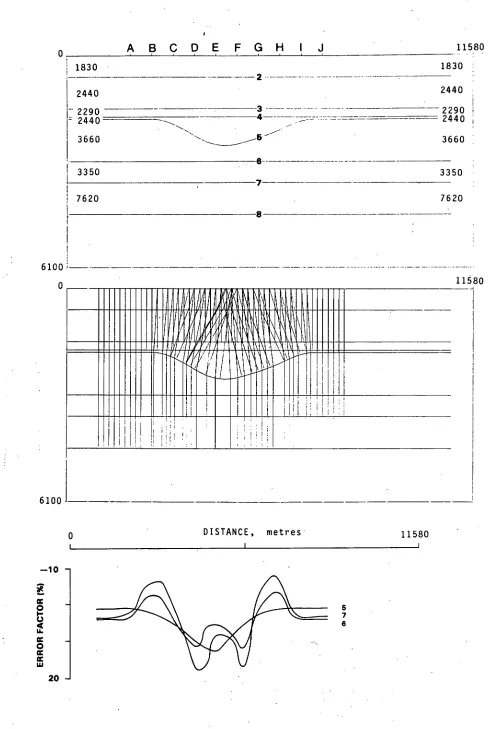
Error factors for surface 5 (Figure 2.16) show a significant increase (10 percent) above the channel base. The asymmetry ol the error-factor curves results from the different side dips of the channels. Time-difference plots (Figure 2.17) show that migration problems become significant on the channel sides [gathers at D (4270 m), G (5490 m) and H (6100 )]. Raypaths for these gathers pass through a

smaller section of the channel fill than would be expected if the CRP was vertically below the gather location, so stacking velocities are large and error factors increase across the channel. Inspection of the zero-offset raypath plot (Figure 2.16) for surface 5 with a gather at location E indicates three potential CRP's. Figure 2.18 illustrates gathers for the three CRP's for this location, while the time-difference plot shows that although there is little error in determining the vertical traveltime, the far traces arrive much earlier (up to -20 msec across the gather) than the near traces and consequently have higher stacking

0 A B C DEF GH I J 11580

1830 1830

2

2440 2440

3

12290 ₄ 2290

-- 4110 4110-

2740 _--- 2740

0

3350 3350

7

8

6100

0 11580

111

1

011111111

III

41

41,819r/Uli MINIMA II 11 I

4"

1114

1

1

111141

DISTANCE, metres ₁₁₅₈₀

6100

6

5

8

50 -

Fig. 2.17 Gathers and time-difference plots for selected locations along the surface of the high -velocity fill-channeI model 'for surface 5. Solid lines - represent the fixed spread. — •

•

9

2.33

Large oscillations of the error-factor curve for

surface 8 are typical of the effect of raypath problems due to the channel fill. The gather at A (2440 m) (Figure 2.19) shows very little migration error, but the far traces

arrive some 40 msec earlier than for the horizontal case

(Figure 2.20). Shifts in the CRP are necessary to accommodate the distortions produced by the far traces passing through the channel edges. Error factors of the order of 45 percent

result. At C (3050 m) migration problems for the zero-offset trace result in timing errors of -25 msec and the raypaths (Figure 2.19) occur as two distinct packets due to a large shift of the CRP. Again the far traces arrive sooner than expected, but the middle traces arrive later giving the gather a "banana bend" appearance.

The converse situation applies to the gather at location F (4880 m). The near traces, which travel through the base of the channel fill, arrive earlier than expected, while the

far traces (Figure 2.19) which pass through the channel sides and hence a smaller section of the channel fill, arrive later than expected. Time differences of 20 msec occur

between near and far traces (Figure 2.20) resulting in

low stacking velocities and negative error factors. Migration errors are small for this gather.

Error factors for horizons below the channel exhibit

2.34 lead to more significant errors because of the small NMO

associated with deeper horizons.

Large oscillations of the variation-factor curves (Figure 2.21) for surface 8 (Figure 2.16) depict the

significant effect of the raypath problems due to the channel fill. The errors for the gather at A are relatively small but increase for large offsets and the long spread due to

the earlier arrival of the far traces (Figures 2.19 and 2.20). Variation plots for the two spreads at location A show

discrepancies of between 5 and 10 percent (Figure 2.21). The large inaccuracies result from the much earlier arrival

of the traces as shot-receiver distance increases (Figure 2.20). Changes occur in variation factor of up to 14 percent for

the short spread and 8 percent for the long spread due to increasing offset.

Time-difference plots and gather plots at D and F show that the near traces which travel near the base of the channel fill arrive earlier than expected while the far traces,

because they pass through the channel sides and hence a

smaller section of the channel fill, arrive later than expected. Consequently stacking velocities are lower than rms velocities and variation factors are negative. Migration errors tend to be minimal. There is little variation in stacking velocity with offset for both spreads.

Variation factors for gathers at I and J are similar to those on the opposite channel side, except for the effect of the slight steeper channel side. These gathers are character-ised by large variation factors and large differences in

/ '

'I

/W/V

/

/ ,

, .

---'', _----

mounn

1111,11/

‘7

41

_\iff

-

r

0 GEOMIONE LOCATION, m 2190

Fig. 2.18 Gathers at E (4570 m) for the high velocity fill channel base illustrating non-zero offset raypaths for CRP's at A, B and C. Time-difference plots are also given.

A

30

20

10

VARIATION

FA

C

TO

R,

%

0

SHOT-RECEIVER DISTANCE, metres

Fig. 2.20 High velocity rill channel time-difference plots for surface to. Solid line represents the fixed spread.

\

2440B

--- --- _________

,., 6700 I 2440B 7320J

7320J

67001

1830A

1830)k•

5490 G

5490G

41.4 227700.B 1100

OFFSET, metres

Fig. _{1.:.21 High velocity fill channel variation-factor} plots illustrating the percentage deviation of the stacking velocity from the rms velocity as a function of offset distance for a short spread (dashed lines) and a long sprea6 (soliC. lines) at selected gather locations.

-id

2.37 (b) Low velocity channel fill

The zero-offset raypath plots (Figure 2.22) for the buried low velocity channel fill show migration of the CRP

for horizons below the channel to be opposite to that for the high velocity fill model.

Error factors for surface 5 indicate trends similar to • the high velocity fill channel and show a 12 percent increase over the channel base.

For gathers above the channel sides sampling of a smaller portion of channel fill than would occur for a vertical CRP results in migration errors of up to 190 msec (Figure 2.23). Raypath plots for gathers (Figure 2.23) illustrate this trend. The gather at F (4880 m) demonstrates a curious effect.

Here the far traces arrive much later than one would

expect, thereby making the stacking velocity lower. Because the zero offset ray arrives 70 msec earlier than a vertical ray, velocity determination by least squares line fitting of a T 2-X 2 plot will result in an excessively large stacking velocity.

Error factor trends for horizons deeper than the channel base tend to mirror the curves for the high velocity channel fill case. Comparison of zero-offset raypaths (Figures 2.16 and 2.22) for deep horizons indicates that for a high velocity channel

0 DISTANCE, metres 11580

5 7 6

0 ;

BCDE

1830 • 1830

_

2

2440 2440

— 2290 3

4 ' 2440

3660 3660

6

3350 3350

7

7620 7620

8

11580

—10 — 6100

6100

2190

CISOPHONI LOCATION.

Fig. 2.23 Selected gathers and time-difference plots for surface 5 for the low velocity fill channel model. Solid lines represent the fixed spread.

OIMPNONII LOCATION rn ₂₁₉₀

Fig. 2.24 Selected gathers and time-difference plots for surface 7 for the low velocity fill channel model. Solid lines represent the fixed spread.

0

—ZOO

!Illi

ll

41

1

-, I

I,

F

_I

_I

i

Hild i

,

■

...,,,,._

.'41/,/,/

2.40 more low velocity fill material, while the far traces

show a relative time decrease from travelling through a

larger proportion of the higher velocity underlying material. The main effect on the gather at D (3660 m) is a -30 msec difference between the zero offset and vertical traveltimes. Arrivals at the far traces are slightly earlier than for the horizontal case because the rays pass through more of the higher velocity underlying channel base material.

The earlier arrival of the far traces is more pronounced at locations E (4270 m) and F (4880 m) where up to 20 msec difference occurs across the traces.

Offset and spread length variation factors for horizons deeper than the channel base tend to mirror (positive curves are now negative) the curves for the high velocity channel fill model. Variation-factor curves for surface 7 (Figure 2.25) are similar,for both long and short spreads despite large overall inaccuracies in velocity determination over the channel.

These examples indicate that accurate velocity

determination of horizons at depth in areas of buried channels is far from easy and probably rarely achieved in normal

processing. When such models are contrasted with typical "simple" geological sections it may be readily appreciated that substantial errors are inevitable.

5. SYNCLINE

2.41 similar (in many respects) to those from the channel base in the previous channel-fill model. Zero-offset time plots illustrate the defocussing effect of synclines and the associated migration problems.

Error factors for surface 6 show large (5 percent) variations across the structure. Even the gather at A (1220 m), which is over an essentially horizontal section, shows variations due to the overburden geology (Figure 2.27). A slight but distinctive "banana bend" occurs;

traces with an offset of 1550 m or less show an increase in traveltime associated with a slightly slower return path on the synclinal base side. Beyond this distance a slight shift of CRP causes a relative decrease in traveltimes. As gathers move towards B (1980 m) the far traces arrive

much earlier than in the horizontal case, resulting in higher stacking velocities and larger error factors. By D (3660 m) migration errors are large (-65 msec) and the far traces arrive earlier than would normally be expected for the horizontal case, further increasing the error factor. At F (4570 m) migration errors are reduced, but the far traces still arrive much earlier than expected and once

again the error factors are large. The time-difference plots (Figure 2.27) show that migration errors are greatest on the slope of the syncline. The relatively early arrival of the far traces becomes more pronounced as the syncline is crossed, thereby increasing error factors.

The variation-factor plots (Figure 2.28) show a 12 percent • range across the syncline. These plots indicate that the

3

3666600 DD — 1830 A

6100 H

618310 0 0 A H

6700 I 3050C 3050C 6700 I

■•••••••

4270E

20

--- 4270E

15

10

Mt

5

4

4 a

0

-5

-10

••••••••••

0

OFFSET, metres 1100

A