Development and analysis of a fluid power test facility

DEVELOPMENT AND ANALYSIS OF A FLUID POWER TEST FACILITY

by

I.F. Jones B.Sc., B.E.(Hons.)

Submitted in partial fulfilment of the requirements for the degree of Master of Engineering Science in the Faculty of

Engineering, University of Tasmania, Hobart.

January, 1972

Abstract

Introduction

Chapter 1 - Hydraulic Circuit and Instrumentation

1.1 Basic Hydraulic Circuit

₅

1.2 The "System"

₉

1.3

1.4 Instrumentation 13

Chapter 2 - The Four-way Valves

2.1 Valve Mk I 22

2.2 Valve Mk I Modified 24

2.3 Valve Mk II 25

Chapter

3 -

3.1 Flow Equation 32

3.2 Flow Reaction Force 34

3.3

₃₇

Chapter

4 -

4.1 Hydraulic Vibration Testing Machine Models

53

77

4.3 Experimental Results 109

Conclusions 130

Appendices 135

Abstract

The work described in this thesis was undertaken as part of a

project to design and build an electro-hydraulic vibration testing

machine of unusual configuration using the limited manufacturing facilities of the departmental workshops of the Engineering School of the University of Tasmania. A sketch showing the basic concept of the

vibrator design is shown in Chapter 1.

Technical limitations concerning available means of measurement and manufacture resulted in the development of a series of four-way spool valves featuring thin axial flutes milled in the spool lands to limit the area gradient and allow ,a long stroke relative to the flow rating of the valve.

An experimental rig to measure spool forces and flow

characteris-tics under various static and dynamic conditions is described in detail.

Difficulties experienced in the operation of the rig are discussed together with suggested lines of rig development.

Digital simulation of hydraulic servo-mechanisms by the Runge

Kutta technique is examined in detail particularly with respect to

the causes of numerical instability. An alternative approach based

on the Method of Characteristics is also described and found to be

particularly useful for systems containing long pipelines. The latter

method is based on the velocity of pressure propagation in the fluid

media and the results of an experimental investigation to determine

this velocity as a function of pressure in a flexible high pressure

hose are presented.

INTRODUCTION

In essence this thesis describes the first attempt by the

Engineering Department of the University of Tasmania to enter the field of fluid power; in particular the field of high pressure oil power transmission and control. As such it possibly contains much rudimen-tary material. However this is included mainly as a background for those at a similar stage of development, or for those who follow.

The project had as its general aim the development of a variable flow, high pressure test facility to which hydraulic components and systems can be connected. However, as with any developmental project, it is preferable to have a more specific goal to work towards. This was the design and construction of a vibration testing machine to be

used for testing machines and structural components. It was to be a

small, compact unit consisting of an hydraulic servo-mechanism

amplifying the output from an electromagnetic exciter. The frequency range was to be from 5 to 250 Hz and the output was to approximate a sinusoidal waveform with low distortion. Furthermore the unit was to be capable of high force levels, the force approaching 5000 lbf at the

lower frequency limit.

With this specific aim in mind, it was therefore of considerable (1) interest to find a French design of vibration testing machine 5

shown below, which was very similar to that envisaged. The article accompanying the diagram however, gave very little useful information about the design or construction of the device. Nevertheless it was decided to aim for a final design very similar to this. This

decision ruled out the use of commercially available four-way valves for the control valve, and as a consequence the Engineering Department embarked on the development and construction of its own valve designs. At the same time the overall analysis of the servo-mechanism was

Cylinder

Driving

ehambers

DC coil oe, Low pressure outlet

A-C coil _{Valve epioel}

Main piston

•

•

-peessure inlet

The analysis of such a servo-mechanism is of course in no way new.

As long ago as 19 47 Coombes analysed a similar system. But, because (2)

of the difficulty in solving the equations which result from assuming a

sinusoidal valve input, he used the rather interesting approach of assuming a sinusoidal output and deriving the required valve input.

(3)

Hoyle had more success by solving the problem with a sinusoidal

input for a simple servo-mechanism without feedback and with an

incompressible fluid. He obtained a series approximation to the solution

which was valid under certain conditions. However when he added

feed-back, the increased complexity forced him to use an analogue computer

(4)

to obtain a solution. Butler also obtained a solution for the

simple servo-mechanism with cavitation by numerical means. In fact

the equations both Boyle and Butler solved were similar to those

discussed in this thesis under the heading of "Solid-slug models".

However Butler makes no mention of numerical instability occuring as

the valve closes; a problem which caused considerable trouble in this

(5)

If compressibility is included in the models the equations

become even more difficult to solve. Consequently most of the models

which include it have been studied with the aid of analogue computers.

( 6 )

Martin and Lichtarowicz used this method to investigate the onset

of cavitation in a servo-mechanism similar to that studied here, but

without feedback. In this project it was unfortunate that a suitable

analogue computer was not readily available. A fast, digital computer

however, was, and consequently the solutions were attempted numerically. _—

This lead to many interesting problems in itself, such as numerical

instability.

Probably the most common method of solution is to linearize the

equations (7 ' 8)

This has the great advantage that the conventional

techniques of control engineering may then be employed in the analysis.

The simple servo-mechanism without feedback was studied in this fashion

(9) ( 10 )

by Reeves while Ashley and Mills investigated a much more complex

servo-mechanism. The latter although not directly applicable to the

servo-mechanism studied in this thesis is of interest because of the

two-stage, flapper controlled valve used to control the ram. Ashley

and Mills showed that the flow behaviour of this type of valve does not

follow the classical dependence on the square root of the valve pressure

drop. In fact the load pressure has only a small effect on the flow;

a fact which could be of some value in a vibration tester. However the

most useful linearization in relation to this project is one by Lambert

and Davies (11). The servo-mechanism they studied is identical to that

in this project and the third-order, linearized model they derive has

been used later to compare with the results obtained by numerically

intergrating the non-linear equations of the system.

The main disadvantage with linearized models, however, is that

the linearization tends to remove some of the distortion in the waveforms.

this respect.

Electric motors

Needle valve

Measuring i tank

Accumulator

Pressur.

gauge

boll valve

Relie; valve

Filter

(i)

HYDRAULIC CIRCUIT AND INSTRUMENTATION

1.1 The Basic Hydraulic Circuit

A schematic diagram of the hydraulic circuit is shown in figure

1.1. Basically it consisted of a pump supplying oil at constant

pressure to a "system" under study. This "system" normally required highly irregularcflows, both of a relatively high frequency pulsating nature and of quite variable average flow rate. The accumulator. was included to smooth out the high frequency pulsations while the variation in average flow was overcome, initially, by the relief

.valve diverting excess oil from the fixed displacement pump back to

the reservoir, and later by a.pressure compensated variable

displace-ment pump. The

supply pressure. TO monitor the supply pressure a Bourdon tube type

pressure gauge was connected to the supply upstream of the "full—flow" ball valve used to isolate the system from the supply.

Reservoir

Oil Cooler Main 14ydrau tic Circuit

Figure 1.1

From the "system" the oil could be taken through a needle valve,

which was used to apply back-pressures to the "system", to a two-way

valve which either directed the flow into the measuring tank or back

to the reservoir. Unfortunately this two-way valve was of the closed

.centre type; an open centre had been ordered but as there would have

been a considerable delay in its delivery a closed centre was accepted. This was a bad mistake for the interruption to the oil

flow as the valve passed through centre caused serious pressure

pulses which not only upset the operation of the "system" but could

also damage the pressure transducers used on the rig, particularly

if, as is anticipated, the supply pressure is increased. It would

be highly desirable to change this valve to an open centre type in

the near

future.

The other main feature of figure 1.1 is the oil cooling circuit

on the left. The cooling was achieved

by

(section 1.3) as it had many interesting

described in detail

features in itself.

The oil used in the circuit was a light "hydraulic" mineral oil

•

(BP HLP65). It hadaddatives for antiwear, antirust, antifoam,

anti-oxidation and a pour depressant. At 100°F the specific gravity was

0.85 and the viscosity 33 centistokes.

Originally the pump, accumulator, relief valve and reservoir

were bought as a complete commercial unit. The pump was a fixed

displacement vane pump capable of pressures up to 2000.psi and a

maximum flow of between 3.5 and

4

pressure from 500 to 2000 psi.

There were several drawbacks with this unit. The main one was

the continuous, constant, high power input required by the fixed

displacement-pump. As this power was dissipated in the oil, it

represented a considerable heat input, and the oil temperature

relatively small maximum flow offered by this pump severely limited the

results that could be obtained. This was very apparent in the early

studies of the valve characteristics, for the valves had been designed

on the assumption of significantly higher. flows.

Late in the project it became possible to purchase a new pump.

The type chosen was a pressure Compensated, variable displacement,

piston pump capable of maintaining pressures from 200 to 3000 psi at

flows up to a maximum of over 6.5 gpm, Fortunately the motor supplied

with the original unit had been excessively large and it was possible

to use this same motor with the bigger pump.

This pump was found to be very satisfactory. Not only was the

maximum flow now of the order of that assumed in designing the valves,

but, because of the variable displacement, the average power input was

greatly reduced, even though the pump was larger. This lower average

power input was due to the considerable periods of time during which

the flow requirements of the "system" were only small. With the

fixed displacement pump this made no difference, for the flow not

required by the "system" was diverted to the reservoir by the relief

valve. However with the variable displacement pump the pressure

compensator shut down the flow, and hence power input, to suit the

requirements of the "system". This usually enabled the oil cooler to

maintain the oil temperature within reasonable limits. The pressure

compensator also meant that the relief valve was no longer really

necessary. Nevertheless it was left on the rig and set to operate at

a pressure approximately 50% above working pressure, which in this

case had been limited to 1000 psi by the original pressure transducers,

to safeguard against any pressure rise due to a malfunction in the

pressure compensator.

Some photographs of the experimental rig are shown in figure 1.2.

These show the rig set up for the dynamic tests on the four-way valve

At the extreme left, the rear of the oil cooler pump can be seen.

(b) The rocker arm can be clearly seen between the valve spool and exciter. The accelerometers are the small cylindrical objects at the end of the valve spool and exciter coupling. The large cylindrical device above tho valve is the displacement transducer.

Figure 1.2

1.2 The "System"

Up to.the present, the Y'Systet" has in the main, consisted of a four-way valve, described in detail in Chapter 2. As such the lt syst em U

was rather ill-defined with respect to the hydraulic circuit, for this

changed depending upon which valve characteristics were being studied

at any given time, To

facilitate these frequent

both within the "system" and to and from the supply. These hoses

were fitted with threaded steel couplings and consequently changes

could be carried out very easily and rapidly.

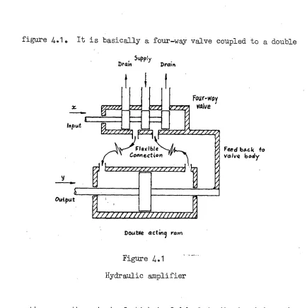
Eventually the "system" will be developed into the hydraulic

amplifier for the vibration tester. This will probably be similar to

the servo-mechanism shown in figure 1.3. In this a four-way valve

Supply brain Drain

Feedback to

valve body

Double 44thiff ram

Figure 1.3

A possible hydraulic amplifier for the vibration tester

controls the motion of a double-acting ram. By oscillating the

valve with an electromagnetic exciter the ram can be made to vibrate

•

1.3 The Oil Cooling Circuit.

Originally it was thought that the heat loss from the pipework

and particularly from the sides of the oil reservoir, might have been

sufficient to maintain a reasonable oil temperature. This also

appeared to be supported by the fact that the manufacturers of the

original unit had not mentioned nor included any form of oil cooling

for that unit. However it soon became apparent that there was almost

no cooling afforded. by heat loss from the pipework or reservoir and

the temperature rose at a rather disturbing rate while the motor and

pump were running. Presumably the painted surfaces of the reservoir

and the fairly still air conditions in the laboratory resulted in a

much lower heat transfer coefficient, between the surfaces and the

air, than expected. In fact an estimate was made of the likely

temper-ature rise assuming no heat loss to.the surroundings and this was found

to agree.reasonably well with the observed temperature rise of

approx-imately 2 F/min. This of course set a severe limit on the length of

run that could be made, for it was observed that for oil temperatures

-

above approximately 190°F, not only did the original pump, the vane

pump, become - excessively noisy but the relief valve also malfunctioned;

it appeared to stick intermittently. FUrthermore, the large

tempera-ture variation during a run caused significant differences to the

results obtained, under what were otherwise identical conditions. The

design of an oil cooler was therefore commenced. This was hampered

by the somewhat vague and.variable information on heat transfer

coefficients and it was no real surprise to find this first design in

error by almost an order of magnitude in heat transfer coefficient.

The design consisted of a coil of 3/8 in. diameter copper tube,

approximately 20 ft. in length, immersed in the oil reservoir. Through

this coil cold water was run. Measurements with this arrangement

showed a very poor cooling efficiency. The heat absorption was only

of the order of a third the heat input and the heat transfer coefficient

was less than 20 BTU/hr °F sqft. It was also noted that the heat

ficient was on the oil side of the coil. With a thermometer it was

observed that a thin, cool, viscous sheath of oil formed over the

coil and even though the oil in the reservoir was kept in constant

circulation by the steady flow of the vane gimp, it was not sufficient

to break up this insulating sheath of cool oil. This could be further

confirmed by vigorously moving the coil in the 'oil, which improved

the heat transfer.

Consequently the circuit was rearranged slightly. A small gear

pump was obtained and coupled to a variable speed motor. This was

then used to pump the oil through the coil,.which was now immersed in

cold flowing water. This showed a great improvement in heat transfer..

Measurements made with this arrangement indicated that the heat

transfer coefficient was approximately proportional to the oil flow,

and a coefficient of almost 100 BTU/111. °F sq ft. was measured at an

oil flow of 1 gpm; very considerably higher than with the coil

immersed in the oil: Unfortunately an attempt to measure the coef-

ficient at an oil flow of 1.5 gpm failed when the light flexible hose -

connecting. the pump to the coil came : off the pump fitting and resulted'

in oil being sprayed all over the room. Nevertheless it was considered

. that this arrangement would be satisfactory until the new pump arrived,

for although it did not remove all the heat being input, it removed

enough to extend the•useful run time by a factor of over three.

A further interesting observation was made with this arrangement.

At low temperatures the oil cooler could very nearly cope with the

heat inflow and the temperature could be kept rising at a low rate.

However when the oil reached a critical temperature of approximately

120 °F, the *oil seemed to rise in temperature much more rapidly and it t

Was difficult to reduce the temperature even by lowering the oil

pressure to below 500 psi. At this pressure the oil cooler should

have coped reasonably well. It could be

that

near the cold tube, wall, being quite viscous, could form a thin insulating

sheath, while the low viscosity hot oil from the reservoir might form

a high velocity jet down the centre of the tube. Unfortunately, as

this was not a primary aim of this project and time was running short,

no measurements were taken to confirm or disprove this apparent change

in oil cooler efficiency. However it is worth noting, perhaps for

future investigation, particularly as the temperature at which

occurs is close to that .at which the rig is usually run, namely 100°F.

This could also seriously upset the operation of any automatically

controlled oil cooling circuit using a similar arrangement.

With the arrival of the new pump the oil cooler was again

modi-fied to try and improve its efficiency. The old coil was cut into

two new coile and these were then coupled in parallel. The reasoning

behind this was as follows. With the same pressure drop across .the

coils as previously - it could not be increased because of the danger

of the hose slipping from the pump fitting - the flow would be increased,

for this pressure now acted across a shorter length of tube. Therefore

provided the heat transfer coefficient kept rising with flow, as

seemed likely from the measurements that had already been taken, the

total heat transfer would be greater, for the two coils together still

had the same surface area, but a higher coefficient. Measurements

taken with this new arrangement confirmed that for the same oil

velocity within the tubes the coefficient was the same. However the

improvement expected was not obtained. The cause of this was the small 0

flow capacity of'the oil cooler pump. The maximum flow, which now had

two paths to flow through, only resulted in an oil velocity within each

tube, of the same magnitude as previously. Consequently there was no

increase in the heat transfer coefficient, and hence no improvement in

efficiency. Of course the pressure drop across the coils had decreased,

but this was of little consequence,.except perhaps, for the improved

safety factor with regard to the hose connections;

This arrangement also suffered from another drawback. The hot oil .

of the cool oil in the reservoir, instead of mixing with it. This was

further aggravated by the oil cooler, for it drew off oil from the

bottom of the reservoir and returned it at about mid-height. Hence

there were two distinct layers in the reservoir; a hot layer at the

top and a reasonably cold layer towards the bottom, with a fairly well

defined interface. An attempt to mix these regions by discharging the

oil from the oil cooler into the reservoir above the oil surface, was

abandoned when it was found that the oil jet, impinging on the surface,

entrained a large amount of air which it was considered desirable to

keep

out

of the circuit.

A better technique would have been to draw

off the oil for the oil cooler, from near the top of the reservoir.

However, when the measuring tank on the rig filled with oil, the level

in the reservoir fell, and consequently the highest point that could

be used was about ' mid-height. Even so, this should have been an improve-ment.

It could be that an oil cooler in the main return line would be

a more suitable arrangement. In any case a new, or at least highly

modified design will be required if there is to be any possibility, at

high power inputs, of maintaining a constant oil temperature. There

is also no reason why it should not be automatically controlled.*

1.4 Instrumentation

1.4.1 Pressure.

Initially a great deal of difficulty was experienced in

obtaining pressure recordings. This was not so much a fault of the

pressure transducers themselves, but more a question of the reliability

of the associated electronic equipment. This was of fairly old vintage

and suffered from very poor drift and noise characteristics. These

transducers also, because of their small pressure range, fixed the

maximum supply pressure at 1000 psi.

* An investigation is currently being carried out on the feasability

of an oil cooler in the pump suction line. This would automatically

control the oil temperature at the pump inlet. Results to date have.

This allowed the experimental results already obtained to be used in

later work. The new transducers were of the diaphram-bonded strain

gauge type (MB Electronics Model 510A). But unlike others, which

required external bridge and amplifier circuits, these were completely

self contained. Built into them was a d.c. bridge circuit with

temper-ature and power supply compensation and a high gain d.c. amplifier.

The pressure range Was from 0 to 2500 psi (absolute), and the drift

and power supply compensation was excellent. No data was supplied

by the manufacturers on the dynamic performance of the transducers,

but this is expected to be more than adequate, as the electronics

um.amm.%

is all d.c. and 'the resonant frequency of the diaphram assembly is

stated to be greater than 20 KHz.

One of the most annoying aspects of these units, and a major

1

drawback, was, the need to isolate the input and output. This often

proved difficult to accomplish if several instruments were being run

off the same power supply. The reason was that if the output of

another instrument Were displayed together with the output of the

transducer, on, say, a dual beam CRO then it was possible to complete an electrical circuit from the output to the input of the transducer,

via the common earths on the CRO and the electrical circuit of the

other instrument. To overcome this, small, individual, floating

output, power Supplies are to be made for each transducer.

1.4.2 Flow

Although no flow meter as Such was used on the rig, average flows could be measured by directing the oil into a measuring tank

and timing a given level change. The oil level in the tank was

indi-cated by means of a clear plastic tube fixed to the outside of the

tank and connected to the inside at the top and bottom. However this

only showed the correct oil level under static conditions. During

flow measurements the oil level was changing continually and

difference between the oil levels in the tank and tube was needed to

create the oil flow into or out of the tube. This difference in

levels was obviously dependent on both the rate of change of the oil

level and the length of tube involved, i.e. on the oil flow and the

oil level. Measurements of this were made, at varying levels, by

suddenly stopping an oil flow into the tank and observing the subse-

quent

rise in oil level within the tube, as the oil in the tank and

tube came to equilibrium. These measurements showed that the

maxi-mum error

1.4.3 Force on the Valve Spool

To measure the force being transmitted to the valve spool

a small, teel rocker arm was incorporated between the exciter and

spool. This can be readily seen in figure 1.2(b). The force was

y effered irom the deflection of the m. To measure the deflection, ar

strain gauges were glued to the upper and lower surface of the arm.

Originally these strain gauges were connected to a commercial strain

gauge unit, which used an a.c. bridge .circuit. However this unit

showed large drifts compared to the forces (more correctly strains)

being measured. The drift was of the order of + 1 lb compared to

the maximum flow reaction force of approximately 8 lb. The unit

also, because, of the low frequency carrier used, had large phase

shifts at frequencies well below 100 cps. It was therefore discarded

and replaced by a d.c. bridge circuit and small integrated circuit

d.c. amplifier. This worked well, although noise from the integrated

circuit tended to be a little large. Later some high gain, high .

stability preamplifiers were purchased and one of these was coupled

to the bridge in place of the integrated circuit. This was found to

be highly sati'sfactory.

1.4.4 Acceleration

Accelerations of both the valve spool and the exciter were

measured with small piezoelectric type transducers (Brael & Kjaer -

•

end of the valve spool and the other to the top of the moving element

of the exciter. The frequency response was limited by the

preampli-fiers coupled to the accelerometers (Brilel & Kjaer - type 2622) and

was flat within + 005 dB from 2 Hz to 10 KHz. These preamplifiers

also scaled the output to 10 Oh (g is the acceleration due to

gravity). Besides being used to measure the accelerations, these

accelerometers were incorporated in the feedback loop of the

vibra-tion exciter control. This is described later in secvibra-tion 1.4.6.

1.4.5 Displacement

In the static tests the displacement of the valve spool was

determined by the use of a dial gauge. This however had one fairly

serious drawback. That was, the dial gauge exerted a quite

signifi-cant force on the valve spool and this had to be allowed for in the

force measurements. Unfortunately this was complicated by the fact

that the force-displacement characteristic of this

gauge

from an hysteresis type effect. This caused the force exerted by

the dial gauge to differ depending upon which way the spool had been

moved to a given position. To a certain extent this was overcome

by tapping the valve body with a small hammer (this had to be done

in any case in order to overcome difficulties of valve sticking).

Displacements during dynamic tests were taken with a small

differential transformer displacement transducer (Hewlett Packard

Model 24DCDT 1000). Basically thiS consisted of a . transformer coil

assembly and a small core which, when displaced along the axis of

the coil assembly altered the coupling between the windings of the

transformer. This difference in coupling was used to produce an

output voltage proportional to the core position. To excite the

primary . winding of the transformer a d.c.-powered oscillator was used.

A quite compact, self-contained transducer was produced by

incorpo-rating the differential transformer, oscillator and demodulator all

within the one case. To transmit the valve spool motion to the core

The main disadvantage of this transducer was the very low

frequency of the oscillator. This meant the filter in the output

stage of the demodulator attenuated the output signal rather badly

and also introduced large phase shifts, at quite low frequencies.

To some extent allowance could be made for this as the nominal filter

characteristics and

3

3

frequency the amplitude was approximately one half of what it should

have been and the phase shift was nearly 60 ° . It would be preferable

to have a transducer with a considerably higher internal carrier

frequency.

1.4.6 Exciter and Vibration Controller

The exciter was a conventional electromagnetic unit driven

by a power amplifier (MB Electronics PM-50 exciter, 2250 MB

ampli-fier), It had.a maximum force capability of 50 lb, if air cooling

was employed, and a maximum stroke of + 0.5 ins. The power amplifier

was driven by the output of the vibration controller.

The vibration controller was basically a sine wave signal

gener-ator, the output of which was controlled by a feedback loop (Brael

& Kjaer - type 1025). In this case the output from an accelerometer

on the valve Spool was used as the feedback signal to the controller.

The controller, if necessary, integrated this signal to give velocity

or displacement, and then rectified and filtered it to obtain an

average input. This was compared to a preset level and an error

signal used to control the output of the signal generator. Hence,

this differed from the type of controller usually associated with this

type of vibration equipment in that it only controlled the average

level of the vibration whether this was acceleration, velocity or

displacement; and in no way controlled the actual wave Shape. This

was somewhat of a disadvantage during the dynamic tests on the valve,

for the valve characteristics caused significant distortions to the

•

Normally the controller was used in a mode that maintained a

constant amplitude of only the acceleration, velocity or displacement.

However it also had facilities to enable a cross-over frequency to be

set at which the control changed from one input variable to another.

Either a constant displacement-constant acceleration, or constant

velocity-constant acceleration mode of operation could be selected.

For the dynamic tests on the valve, the former mode was used, i.e.

constant displacement-constant acceleration. The cross-over

frequency was slightly less than

55

frequency range of the controller and exciter combined was from

5

Hz

to 10

KHz, However power requirements limited the maximum frequency

on

1.4.7 Ultra-Violet Recorder and Preamplifiers

For the permanent recording Of most of the measured variables

on the experimental rig a U.V. recorder was used. This consisted

of a number of small galvanometers which deflected, by means of a

little mirror attached to. the galvanometer suspension, a fine spot

of ultra-violet light onto a sensitised paper. This paper could be

driven through the recorder at varying speeds. It was developed in

ordinary light leaving the trace quite visible.

If

provided the paper was stored in a dark place (to stop further

-.development). The response of the galvanometers was flat to 300 Hz

which was quite adequate for most of the signals being recorded.

However some recordings, such as pressure, were so rapid that it was

necessary to use a CRO to observe them, particularly the amplitude,

as the galvanometers attenuated the peaks. The galvanometers were

electrically

damped

the

The preamplifiers were designed and built in the department using

integrated circuits. The original specification was for a d.c.

Feedback

from 0.1 to 10 and impedance matched to the U.V. recorder

galvano-meters which had a resistance of only 120n. It was also to have

very low electrical and temperature drifts. The circuit sketched in

figure 1.4 was built and tested. It was found to be quite

satisfac-tory provided the output impedance of the source driving it was not

too high. The reason for this was that the integrated circuit

required an input bias current of approximately 20 nA. This was

normally only important in the case of piezoelectric type transducers.

Operational

Amplifier

411,-

Rp - protection for galvanometer

- damp;ng resistance for

lalvanometer

Figure 1.4

Galvanometer preamplifier

However, some of the equipment it was anticipated using with

these preamplifiers was found to have a large d.c. offset voltage of

the order of 11 V. Consequently the specification had to be

modi-fied to allow a.c. coupling at the input and this, in fact, caused

very great problems. This was because of the bias current required

by the input stage of the integrated circuit. With a capacitor

coupling between the source and .input the only means of supplying

this current was via some form of bias resistor circuit. But the

specification required an input impedance - of greater than 1 M12.

itp Rd

IKA

Galvanometer

bias current was approximately 20 nA the voltage offset across this

resistance was then 20 mV. This was quite large compared to the

input signals expected. An idea of their range can be gained by

observing that the galvanometers required only about 60 mV for full

scale deflection and even at the lowest amplifier gain of 0.1 this

represented only 600 mV at the input. Relative to the smallest

signal expected the offset was a factor of three times larger! The

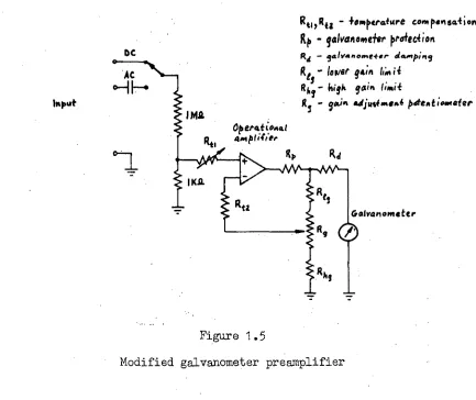
final compromise arrangement is shown in figure 1.5.

Input

DC

AC

HE"'

I MA

Operatienuti

emplWer

Rt,,Riz - temperature compensation

Rp - qalvanowlefer profettion

Rd - lolvono..e.tfir damping

Rts - lower qe;n Isii R1,1- high gain

- adjus4me..4 keteetimmefer

•

•••

Figure 1.5

Modified galvanometer preamplifier

This was only moderately satisfactory because of the large

attenuation of signal at the input. This meant the signal being fed

to the operational amplifier was becoming comparable with noise and

consequently at gains greater than about 5 the noise at the output

became excessive. A further problem was that the circuit could only

be temperature . compensated for either d.c. or a.c. but not both as

the impedance'seen by the input to the operational amplifier was

the offset on switching from d.c. to a.c. it did not overcome the

problem and consequently the trace had a quite considerable offset

on switching over.

Nevertheless as a considerable amount of time

had

been spent on this design it was decided

with it.

It

reasonably priced commercial unit, which would satisfy the specifica-

tion,

but as yet none has been 'found

that

would be entirely

satisfactory.

CH.POT

THE FOUR-WAY VALVES

2.1 Valve Mk I .

At the time this project was comme ed a four-way, spool Valve

was already under construction in the dep tmental workshop. It had

a three land type spool as shown in the det 1 drawing, figure 2.1.

Essentially the valve consisted of three part..- A mounting flange and

outer body which had the threaded holes for the high pressure hose

fittings, an inner sleeve in which the valve pox' were machined, and

I

finally the valve spool itself. As it was not expe ed that a long

component life would be required, in the first valve design anyway, all

components were made from mild steel. This also meant they could be

easily machined. The close radial fit between the spool and sleeve

was achieved by first making them with a slight interference fit. The

sleeve was then honed and finally thespool and sleeve lapped. A

‘•

feature of this design was the ease with which it could be dismantled \.

or altered. Considerable modifications tO the valve characteristics, or even style, -could be made by siinply'machig' a new sleeve and spool.

An examination of this first valve design however showed that it

had many faults. The most obvious one was the asymetrical nature of

the valve ports (see section through sleeve, figure 2.1). With a-

supply pressure of 1000 psi . it was anticipated that the valve would

lock in the closed position due to the large side thrust caused by this. There was a.probleml too, of the end lands of the valve spool

fouling the drain holes. These drain holes had already been moved in

order to clear some "0" ring seals that had been placed between the

sleeve and body!. Farthermore a quick estimate of the flow characteristics

of the valve showed that the maximum flow would be developed at a

displacement of- only about 0.01 in. This Was thought to be somewhat

small for accurate measurements within the laboratory and particularly

•

lands. Nevertheless it was deeided to perservere with the fabrication

of this valve so • that the overall assembly of the hydraulic rig would

not be delayed. It was also expected that the experience gained, not

only in the manufacture of the valve components but also in the

opera-tion of the hydraulic rig ) would be of great benefit in later valve designs and experiments. At the same time, possible modifications to this valve were investigated in an attempt to see if some of these

difficulties might be overcome fairly simply. As well as this the

design of a completely new sleeve and spool (Valve Mk II) was

commenced.

As predicted, when the valve was tested on the rig, it was found

to lock as. it passed through centre. It could only be moved with a

great deal of difficulty and very large forces. Also the full flow

was reached within a very small valve travel as had been expected.

The leakage on the other hand appeared to be fairly small which was a

Very encouraging result.

2.2 Valve Mk I Modified

In order to overcome the large side thrust on the valve spool of valve Mk I, two more slots were cut around the valve sleeve at the central port position, as shown in figure 2.2. This balanced the

Figure 2.2

Section through central port of

pressure forces around the spool at this position. Unfortunately this

could only be done on the central port as the resultant slot at the

other two port positions would have touched the leakage drain holes!

In any case, as the design of the new spool and sleeve was

_well

advanced it was decided to concentrate on the central port only, and

see how it behaved.

The valve was reassembled and connected to the high pressure

supply. Tests on this modified valve proved reasonably satisfactory

as far as the

However the pump could only manage to maintain 600 psi or less across

the valve, even in the fully closed position. It was suspected that

the majority of the flow was in fact leaking around the central land

of the spool, but at the same time it was thought some might have been

leaking between the sleeve and body. In order to determine just how

important this leakage around the sleeve was, the valve spool was

partially removed from the sleeve so that the large end land completely

blocked', the central port. The high pressure oil was again connected

---and the total leakage found to be very small, indicating that for all

intents and purposes the flow previously observed was all past the

central land.

A quick analysis of the flow and pressure drop showed that a

valve underlap of some four thousandths of an inch was required.

Consequently the valve was dismantled again and the sleeve and spool

carefully examined. This Showed that although the slot width and

spool land dimension Were very nearly identical, the two extra slots

that had been cut around the sleeve, were axially displaced by several

thousandths of an inch from the original slot. This together with the

small radial clearance was sufficient to account for the results .

observed (remembering that the port width was now three times larger).

2.3 Valve Mk II

It was decided if possible, in this design, to use the existing

-

it severely limited what could be done with the spool and sleeve. The

main problem was the very large flow obtained at only very small

displacements of a conventional type spool valve with large port widths.

For this valve it was felt that, for the full pump flow at the supply

pressure, a displacement approaching 0.1 in. was desirable. This was

because the tolerances that could be held on the sleeve and spool were

poor relative

normally maintained in this field. Also, for

accurate measurements of the spool displacement, particularly dynamic

measurements, within the laboratory, a reasonably large displacement .

was necessary. However this meant a total port width of less than

3/16 in.: The problem was therefore to either decrease the spool

diameter and hence port width, in the case of an annular groove type

porty 'or to machine several very small rectangular ports in the

sleeve. For the spool diameter it was decided that the minimum

'diameter that could be handled with any accuracy on the available

equipment was of the order of 0.5 in. or greater. Therefore the

desired maximum spool displacement had to be decreased unless very

small width ports could be made. However the latter appeared quite

difficult as the only convenient way of making a rectangular port was

by slotting across the sleeve, and the tolerances that needed to be

maintained to give the. required port width accuracy, with a spool

diameter greater than 0.5 in., were unrealistic.

By chance, .at about this time, a slotted or fluted spool

construction was discovered. This.had spool lands much longer than

the port size. Slots were then machined in the lands in such a way

. that the end of each slot just touched the edge of the port. See

figure 2.3. This allowed the actual port width in the sleeve to be

large and yet still present an effective port width, for the oil flow,

of just the combined width of the slots in the spool land. The one

major drawback with this technique was the difficulty in locating the

ends of the slots accurately. With this particular valve the problem

was partly overcome by measuring the average position of the ends of

SECT

Va

lve

Mk It

C

RO

S

S

SEC

TIO

Drain Supply, Drain

)

1

L

L/_,L1

1

To double actin, ram

to match. However with later valves which are to be hardened by heat

treatment, any distortion of the spool will result in non-uniformity

of the slot end-positions around the spool, as these will have to be

cut before hardening.

The other main feature that had to be considered was how many lands

to have on the spool. As already mentioned in the discussion of valve

Mk I, if a.three land construction were used the end ports could not

be placed uniformly around the sleeve as the resultant slot fouled the

leakage drain holes. Consequently the only valve spool that could be

constructed that would fit the existing outer body Was a two land type,

'shown in figure 2.3. This was very unfortunate as it left oil trapped

between the end caps and the valve spool. • Normally this type of valve

would be made with four lands as shown in figure 2.4. In this case

Figure 2.4

Conventional four land,. four-way valve - .

there was no room to place the extra two lands and this presented

difficulties in later experiments due to slight pressures built up in

these end chambers. These caused extra axial forces to be exerted on

the valve spool.-

As previously, the spool and sleeve were made from mild steel.

The radial fit was also obtained as before,-i.e. the spool was first

made an interference fit with the sleeve, the sleeve then honed and

- 29 -

were taken of the radial clearance. However the fit was certainly

reasonable, for the leakage flows were small, approximately 1.5% full

flow, as can be seen from the results presented in the next chapter.

In comparison the tolerances actually held on the other dimensions

were not very good. The ends of the slots were within approximately

+ 0.001 in. of each other and there was an average overlap of slightly

greater than 0.001 in. on the high pressure side of the valve lands

and an average underlap of approximately 0.001 in. on the low pressure

side of the lands. As

it turned out this was not very critical, for

the full flow displacement was relatively large, being approximately 0.1 in. Also the slot effective area was not strictly determined by

the displacement of the slot alone but by a throat area which was

also determined by the slot shape, as described in the next chapter. One further feature of the valve was the provision of an axial hole through the centre of the valve spool. This was done in readiness

for hydrostatic bearings on the spool', if these were required later.

This axial hole was to, carry oil from the high pressure. oil chamber to

several small radial holes drilled through the lands, between the slots, as shown in figure 2.5. Restrictions were to be screwed into.

r

ix.* lanai

Nigh pressure

eZ,43

,4

541thion AA

Figure 2.5

Hydrostatic bearing for valve spool.

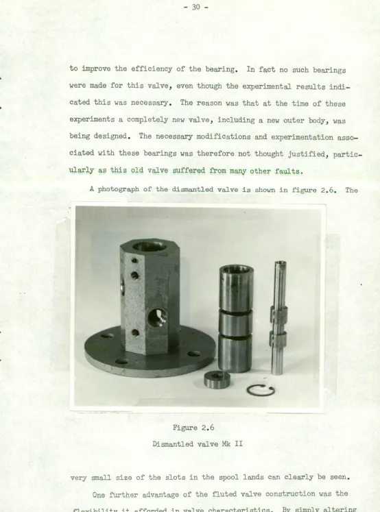
to improve the efficiency of the bearing. In fact no such bearings were made for this valve, even though the experimental results indi-cated this was necessary. The reason was that at the time of these experiments a completely new valve, including a new outer body, was being designed. The necessary modifications and experimentation asso-ciated with these bearings was therefore not thought justified, partic-ularly as this old vnlve suffered from many other faults.

A photograph of the dismantled valve is shown in figure 2.6. The

Figure 2.6

Dismantled valve Mk II

necessary. In fact something of this nature could possibly be used to

overcome problems of cavitation in the hydraulic amplifier of the

vibration test rig.

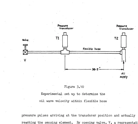
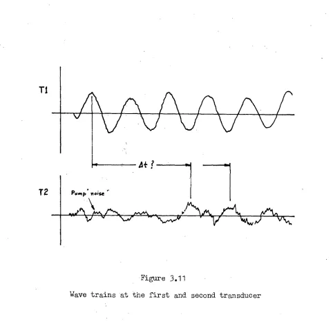
kfurther point of interest relevant to this section is the orifice

flow nomograph presented in appendix 1. This was found to be extremely

useful throughout the project.. It allowed very easy rapid estimates of

the flow behaviour of orifice-like restrictions to be made, and this

was particularly handy during the valve designs.

computer program was written to produce the nomograph on the digital

incremental plotter coupled to the Elliott 503 computer at the

University. The program procedures or subroutines which were used to

plot the axes were written fairly generally so that almost any

nomo-graph could be produced with a minimum of time and effort.

CHAPTER 3

STATIC BEHAVIOUR OF THE VALVE

3.1

Flow Equation

If "steady-state" conditions are considered to exist within the

valve and the flow in the vicinity of the metering orifice is incom-

pressible,

_{non viscous and turbulent, then the flow will follow the}

"orifice" equation:

where Q = rate of flow .

Cd = discharge coefficient

•

A =

• Sp = pressure drop across valve

• f = oil density

That this equation does in the behaviour of most valves of the type being considered here, i.e. valves with a . large

pressure drop. across an orifice type restriction, has been shown by

many workers in this area(78, 12) . Indeed, as will be shown later

in this chapter, the valve studied in this experiment was no exception.

In general the discharge coefficient, C d , is taken to be constant.

This is not strictly correct, particularly for very low pressure drops

or small valve openings (12). However other effects are usually much

more important than this in causing discrepancies between the measured

and calculated flows, and for most valves the assumption of Constant

C

d is very good. This was certainly true of the valve studied in this

experiment. For an orifice with sharp edges a coefficient of 0.6 - 0.65

is usually observed; for slightly rounded edges it is 0.8 - 0.9 and

varies somewhat. In respect to the fluted valve the metering orifice .

had as well as sharp edges a reasonably smooth flat "edge". See

figure 3.1. Therefore, for design purposes a coefficient of 0.7 was

assumed. This turned out to be close to the value actually measured,

60

el X 2 0. 52

.

_

8

KO .120 .

actual displacement (0.001in) Figure 3.1

The valve metering orifice

A further point that needs examining more closely is the

relation-ship between spool displacement and orifice area for a fluted valve

spool. In the more conventional "square raand" type. spool valve the

orifice area is simply , .the product of the displacement and the port

width. However with the fluted design there is in fact a "throat" of

Considerably smaller area than the displacement times the port width.

This is clearly, shown in figure 3.1. Moreover this throat is not a

linear function of the displacement of the spool, as shown in figure 3.Z.

Figure 3.2

In this figure an effective displacement has been obtained by dividing

the throat area by the port width (strictly speaking, by the combined

slot width). This is the equivalent displacement that would be required

to give the same orifice area with a ttsquare_landtt spool. Figure

however, also shows that over the range of displacements expected, i.e.

displacements upAo 0.1 in., the effective displacement can be

approxi-mated quite well by

X

ec a c.4

where k = 0.52 approximately, for the valve considered

here.

In general k will be different for different valves and displacements.

The orifice area is therefore given by

A=kwx

where w = port (combined slot) width

and the flow equation becomes

C

d kW 3C.1?-61-

f

4.4 As this equation is used later in deriving the equations for the

dynamic behaviour of the system, it is perhaps pertinent to comment on

the meaning of the 'steady-state" assumption, originally used in deriving

these equations. In the dynamic situation, steady-state conditions can

not in reality be said to exist. However it is assumed that the speed

with which the flow in the vicinity of the metering orifice changes,

due to variations in the upstream or downstream pressure, or due to

changes in spool position, is very much more rapid than the speed with

which these "external" changes occur. Hence at any instant during

changing conditions the flow through the valve is assumed to be the same

as the flow that would have resulted had

tho

spool position existed during steady-state conditions.

3.2 Flow Reaction Force

Consider the schematic diagram, figure 3.3 showing one metering

Valve

spool

Figure 3.3

Section through spool valve

through duct B. In general the areas of the ducts and the chamber,

are large compared to the area of the orifice and consequently the

velocities are small with the exception of the velocity of the oil jet

passing through the orifice. This jet is not only of high velocity

but it enters duct B. at an angle, e 900_{, and therefore carries away}

some axial momentum. This it could only have, gained from the "spool"

chamber and consequently there must be a reaction force onthe spool

which tends to close it. This is very briefly the Origin of the flow

reaction force.

Referring back to figure 3.3) provided the angle of the jet, 6,

is known, the axial force on the spool can be calculated. This force

'must be the net axial component of the rate of change of momentum of

the oil passing through the valve. Because the velocity of the oil

entering the chamber is very small compared to that of the jet leaving

it, the momentum flux entering' the chamber is usually ignored. The

momentum flux, MI leaving the chamber can be determined at the vena

contracta of the jet. It is

where v_{2 —} - velocity at the.vena contracta.

By the Bernoulli equation

The axial force, Fp _{is given by the net axial change in momentum}

--- flux, i.e.

F

Combining this with the flow equation (3.2) finally gives

F

----a

C

d

K w x

If the direction of flow is reversed so that the jet flows into,

the chamber from duct B, the equation still holds and the force still

tends to close the valve.

For a "square-land" valve when the valve opening, x, is small

compared with the Other dimensions of the chamber, but large compared

with the radial clearance, the angle, 6, is found to be approximately

69o (12)

was nowhere near square l -the.angle.being about 350 as shown in figure

11

3.4.

. •

these angles, probably closer to 350 than 69° due to the effect of

Port

Figure 3.4

Spool land edge angle

the slot on the flow'. As Shown later, the angle in fact was

Stlpply Back press/4u

valve

MeaSurms 'Fmk

1

—X

30 Experimental Results

3.3.1 Pressure-Flow Characteristics

Because of the peculiarities, of valve Mk II, particularly

in having only two lands, instead of the more usual four, it was

difficult to find a satisfactory way of coupling it to the rig, The

most satisfactory method seemed to be that sketched in figure 3.5.

However even this had the disadvantage that any difference between

Drai

Figure 3.5

. Hydraulic circuit for static tests

the oil pressures at the measuring tank and return line caused a

resultant force on the spool as these pressures were communicated to

the chambers between the end-caps and the spool lands. FUrtherMore

the leakage flow measured when the valve was closed was that across

the whole land, not just from the high

pressure

Fortunately this was not a very great disadvantage in this case as the

only occasion for which the leakage flow could be measured was for.

"zero" back pressure. In all other cases the tack. pressure could not

be maintained with only leakage flow, as the outside edge of the land

opened the port to the end chamber and hence zero pressure. In any .case,

with "zero" back pressure . the - major part of the leakage flow should have

been from the high'pressure edge of the land to

the port as the.pressure

(Strictly speaking this was not quite correct, for the 'port did not

extend continuously around the sleeve and consequently between port

sections there would have been a slight pressure build up).

The "outside" land Characteristics, i.e. the characteristics from

the port to the end chamber, were net studied in this particular experi-

ment.

character-istics across the "inside" lands were required for the dynamic studies

• anticipated with this particular valve. Secondly, as a result of the

two land construction, the results obtained for the "outside" lands were

: expected to be somewhat unreliable. This was because of the slight

pressure increase that would have been created in the end chamber due

. to the oil flow through it. This would have upset the flow reaction

'force readings .. .Also'the-large clearance between the .end-cap and the

• valve spindle would have resulted in a significant leakage flow pastthe

end-cap.:

• One further point that should be made about this valve is that the

characteristics of anymetering orifice cannot be assumed to remain

the same if the directionof oil flow is 'reversed. In fact it is very

likely that there willbe.a difference, for in one case the oil flows

• .through a convergent slot and throat into a fairly large duct, while for

the reverse flow,-the oil passes from the duct, through the throat into

a divergent slot. In all that follows the "inside" land characteristics

are considered for an oil flow out through the spool slots to 'the duct

or port.

. The raw data obtained from valve Mk iI,.with . a supply pressure, of

1000 psi, is shown plotted in figure 3.6. Positive flows were taken to

be flows through one port, while negative flows were through the other

port. At small flows the plots are reasonably linear; however at

higher flows there is a marked roll-off or saturation effect as it is

commonly called. At least some of this roll-off cah. be considered to

be due to pressure drops within the hoses and fittings both upstream

and downstream Of the valve. These caused a drop in the total.pressure

t_ =

en

Li-

stage, in assuming the total roll-off to be due to this cause, as the

valve need not have been linear. Indeed this Was one reason for

actually measuring the valve characteristics). With one exception the

hoses and fittings upstream of the valve were large and should

have

offered

only

a small resistance to the flow. The exception was at the

entry to

upstream of the valve, it was assumed that, as the e in. hole was the

most significant restriction, it caused mostof the pressure drop.- It

was then assumed to behave as a sharp edged orifice of the same

diameter.

Downstream of the experimental valve the oil had to flow through

several fittings and valves. However in this case the pressure drop

was measured directly by a pressure transducer placed just downstream

of the experimental valve. This made it possible to calculate an

equivalent orifice type restriction to represent the loses downstream

of the valve. It should be noted, however, that this was only

applic-able to the "zero" back pressure results. ( Strictly speaking, even

though these results were obtained with the back pressure valve fully

open, the back pressure was not zero due to the pressure drops down-

stream). For all other results the back pressure was maintained constant

by the back pressure valve irrespective of the ail flow. The hydraulic

circuit therefore looked somewhat like

figure 3.7

figure 3.7 (b)

•

•

Upstream Restriction due to restriction back preside valYf

Experimental

SuppIr pree. Valve ..••••••\ Drain pras.

(a)

Ups+ /vain

resfriction

ExPerimentel Valve

suPtlY l'•u. Back pres.(torestarri)

( 3 ) Figure 3.7

Hydraulic circuit for (a) "zero" back pressure,

C k w (x+x

ThiS explains the greater droop in the "zero" back pressure curve; the results in this case. had the added effect of A flow dependent pressure drop downstream, as well as upstream. The estimates of the pressure

drops upstream and downstream of the valve were used to evaluate the

approximate pressures that actually existed acrossthe metering orifice

of the Valve at any flow. This, together with the assumption. that the

valve behaved, at least to . a . first approximation in accordance with the

orifice equation (3.2), enabled a Correction to be made to , the flow

results to give an estimate of the flows that would have resulted had

there been no pressure drops Upstream or downstream That the valve

did behave, at least.t0.a first approximation, in accordance with the

orifice equation, can be 'deduced from the resultsalready presented- in

figure 3.6. In addition to this correction; a small correction was made

for the non-linearity of the orifice area with displacement. The

"corrected" results are plotted in figure 3.8. There-is:stiil .a small ,

'amount of roll-off at the higher flows. This Could no doubt be

elimi-nated by assuming:slightly higher losses. However this is hardly

justified in view of the assumptions, and estimates already made to

obtain these curveL. In new valve designs, one of Which is presently under construction, Provision has been made for pressure tappings into the valve body,to'enable the pressure drop across the metering orifice

tobeacCUrately measured.

Figure 3.8 also shows that the Valve wad . slightly•under lapped,

theextrapoIated flow curves reach zero flow l ignoring leakage, at

a small negative displacement, x This is'taken'into account . in -

some of the mathematical models. presented in chapter . 4 by displacing the Origin of the orifice flow equation as below:

The results presented in figure 3.8

( 3.4)

also Show that,. with the exception of •

the 600_ psi back pressure set, the coefficient of discharge is very nearly constant. The average value, excluding the 600 psi results, is

•11,

-43-

the case of the 600 psi set and this could explain why the discharge

coefficient in that case is lower, at 0.69.

It should be noted however, that these discharge coefficients, and

indeed figure 3.8 itself, do not in reality describe the actual,

physical valve. They represent the behaviour that would be expected

from a valve of similar design to the one discussed here : but

with a

linear displacement throat area characteristic and constant pressure

drop across the metering orifice. In chapter ₄

_results

valve, hoses and fittings, and as such figure 3.6 represents the

behaviour more correctly than this figure. The discharge coefficients

use in chapter 4, therefore, have been chosen so as to best

approxi-mate

the behaviour shown

to show that the actual metering orificev,does in fact behave in

accord-ance with

the orifice

though

physical appearance is

more that of a restricting passage than an orifice.

3.3.2 Flow Reaction Force

As already mentioned, because valve Mk II had only two spool

lands, it was possible that significant errors could occur in the

flow reaction force measurements. These, could arise as a result of

different oil pressures within the chambers between the end caps of the

valve and the valve spool lands (see figure 3.5). In addition, during

the actual tests of the valve, two further effects were observed. The

most significant effect was the valve spool sticking, often called

hydraulic lock, particularly at high back pressures. To overcome this

it was necessary to lightly tap the valve body with a small hammer to

jar the spool free, This tapping, however, could itself introduce

bias into the results as it was found that tapping the side of the

valve body had very little effect; the tap had to be in an axial

direction and in the case of high back pressures it had to be

reason-ably heavy. The other significant effect was the force exerted on

the spool shaft by the dial gauge used tO Measure the spool position.

This was complicated by the fact that the dial gauge force, besides