Reasoning by Term Rewriting
by Michael Bulmer, B.Sc. (ions)
submitted in fulfilment of the requirements for the degree of Doctor of Philosophy
December 1995
I declare that this thesis contains no material which has been accepted for the award of any other degree or diploma by the University or any other institution, and that, to the best of my knowledge and belief, this thesis contains no material previously published or written by another person, except when due reference is made in the text of the thesis.
Abstract
We propose a broad system for reasoning by term rewriting. Our general aim is to capture mathematical and scientific reasoning in a coherent sys-tem. To this end we introduce several new processes which allow concrete descriptions of standard notions.
For deductive reasoning we extend traditional methods for finding canoni-cal rewrite systems to a general method for systems involving both equa-tions and inequaequa-tions. We introduce the notion of side condiequa-tions for non-theorems and show how they provide a new kind of meta-reasoning whereby an automated reasoner can determine why it failed to prove a given state-ment. A method for the automatic proof of inductive theorems by an ana-logue of mathematical induction is also presented.
A new algorithm is given for inductively generating conjectures (function equations) from a set of observations (a rewrite database). This is a process of scientific induction and we prove some fundamental results linking it to mathematical induction. Comparisons are given with standard inductive learning systems, such as FOIL, to illustrate the expressive power of our algorithm.
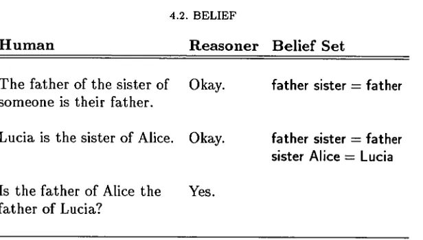
We obtain probabilistic measures of the strength of a single conjecture using statistical testing and an information measure. For a collection of conjec-tures we are then able to quantify Popper's well-known falsifiability criterion for the strength of a theory. We also introduce a non-standard modal oper-ator to extended our deductive reasoning to reasoning with conjectures. We use belief dynamics as the framework of an implementation of the rea-soning methods. Consistency analysis, using the same canonical-form algo-rithm introduced earlier, allows the reasoner to build a belief set from given knowledge and to form a working theory from the conjectures it makes. Again a meta-reasoning is introduced, with the reasoner then able to decide what experiments need to be carried out when it conjectures more than one consistent theory from given set of observations.
Contents
List of Examples
List of Figures viii
List of Tables ix
Acknowledgments xi
Chapter 1. Introduction 1
Chapter 2. Preliminaries 5
2.1. Language 5
2.1.1. Algebraic Definition 5
2.1.2. Categorical Definition 6
2.2. Predicates 6
2.2.1. Entities 7
2.3. Structural Rules 8
2.3.1. Category without Products 8
2.3.2. Category with Products 8
2.3.3. Sets 9
2.3.4. Term Orderings 11
Chapter 3. Proof Methods 13
3.1. Equational Proof 13
3.2. Proving Equations 14
3.2.1. Proof by Normalization 14
CONTENTS ii 3.2.3. Uniqueness of Canonical Rewrite Systems 16
3.2.4. Proof by Invariance 19
3.2.5. Proof by Contradiction 20
3.2.6. Proving Compound Sentences - Conjunction and Disjunction 23
3.3. Proving Inductive Theorems 24
3.3.1. Strong Completeness 24
3.3.2. Inductive Theorems 27
3.3.3. Characterizing Ambiguity 29
3.4. Proving Inequations 32
3.4.1. Proof by Contradiction 32
3.4.2. Proving Compound Sentences - Implication 33
3.4.3. Compound Hypotheses 34
3.4.4. Minimal Systems 36
3.4.5. Proof by Invariance 41
3.4.6. Inductive Proofs of Inequations 41
3.5. Theorems and Possible Theorems 42
3.5.1. Side Conditions 42
3.5.2. Side conditions for Compound Sentences 45
3.6. Abductive Reasoning 47
3.7. Solving equational systems 48
Chapter 4. Logic and Belief 54
4.1. External Truth: Logic of Equations 54
4.1.1. Quantification 54
4.1.2. Consequence Relations 55
4.2. Belief 57
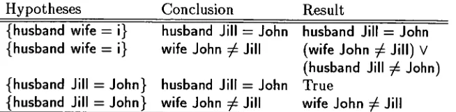
4.2.1. Implementing Belief: Dialogue and Proof 59
4.2.2. Belief Dynamics 62
4.2.3. Contraction 63
4.2.4. Expansion and Revision 64
CONTENTS iii
4.3.1. Meaning 67
Chapter 5. Learning Equations from a Database 70
5.1. Induction Method 70
5.1.1. Facts and Conjectures 70
5.1.2. Induction Algorithm 72
5.1.3. Families and Gender 75
5.1.4. Inductive Generation of Function Inequations 79
5.2. Language Dynamics 79
5.3. Applications 81
5.3.1. Classification 81
5.3.2. Family Relationships 83
Chapter 6. Inductive Belief 86
6.1. Numerical Measures of Conjecture Strength 86
6.1.1. Hypothesis Testing 86
6.1.2. Posterior Measures 88
6.1.3. Predictive Measures 90
6.1.4. Information Content 93
6.2. Consistency and Experiments 95
6.2.1. Closure 95
6.2.2. Competing Theories 98
6.2.3. Inductive Experiments 100
6.2.4. Falsifiability 102
6.3. Blocks World 106
6.4. Theoretical Systems 110
6.4.1. Data Compression and Axioms 110
6.4.2. Toy Physics 112
6.4.3. Theories Concerning Points 112
6.4.4. Theories Concerning Numbers 114
CONTENTS iv
6.5.1. Modal Operators 118
6.5.2. Reasoning with Probability 119
Chapter 7. Conclusion
121
7.1. Dialogue with a Scientist
121
7.2. Concluding Remarks
122
Bibliography
127
List of Examples
2.1 Set reduction 10
3.1 Normalization proof 15
3.2 Lexicographic ordering 17
3.3 Invariance proof 19
3.4 Contradiction proof 21
3.5 Unbounded hypotheses 22
3.6 Non-theorem 22
3.7 Conjunctive conclusion 23
3.8 Disjunctive conclusion 23
3.9 Non-deductive theorem 24
3.10 Unique maximal theories 25
3.11 Multiple maximal theories 26
3.12 Functional completeness with ambiguity 29
3.13 Infinite domain 31
3.14 Obtaining inductive truth with co 32
3.15 Contradiction proof of an inequation 32
3.16 Non-theorem 33
3.17 Proving an implication 33
LIST OF EXAMPLES vi
3.19 Hypotheses with implication 35
3.20 Multiple minimal systems from KBI 37
3.21 Invariance proof of an inequation 41
3.22 Importance of ordering 43
3.23 Non-extraneous side condition 43
3.24 Side conditions from an unbounded non-theorem 44
3.25 Impossible theorem 44
3.26 Side conditions for compound conclusion 45 3.27 Side conditions for compound hypotheses 45
3.28 Impossible conjunction 46
3.29 Hypotheses with implication (revisited) 46
3.30 Abductive diagnosis 47
3.31 Solving a simple system 49
3.32 Solving with inverse functions 49
3.33 Solving with multi-valued functions 50
3.34 Solving an inconsistent system 50
3.35 Solving with redundant equations 51
3.36 Eliminating unknowns 51
3.37 Solving a system with two indeterminates 52
4.1 Simple truth 59
4.2 Side conditions 59
4.3 No information 60
4.4 Impossibility 61
4.5 Implication 62
LIST OF EXAMPLES vii
4.7 Working system 66
4.8 Meanings of conjunctions 68
4.9 Internal proof 69
5.1 Refinement of conjectures 75
5.2 Consistency of conjectures 76
5.3 Finite induction and infinite deduction 77
5.4 Recursive conjectures 77
5.5 Facts from infinite domains 77
6.1 Consistent subsets 96
6.2 Two competing theories 99
6.3 Three competing theories 99
6.4 Conflicting predictions 101
6.5 Three conflicting predictions 101
6.6 Extraneous result 102
6.7 Predicate theory strength 104
6.8 Equal theory strength 105
6.9 Multi-sorted theory strength 105
6.10 Simple learning in a blocks world 106
6.11 Working theories in a blocks world 107
6.12 Conjectured axioms 111
6.13 Probable truth 120
6.14 Answers from probable information 120
7.1 Dialogue with simple answers 121
List of Figures
3.1 Motivating family tree 16
5.1 Adam and Eve's family tree 78
5.2 Visual data for classification 82
5.3 Two isomorphic family trees 84
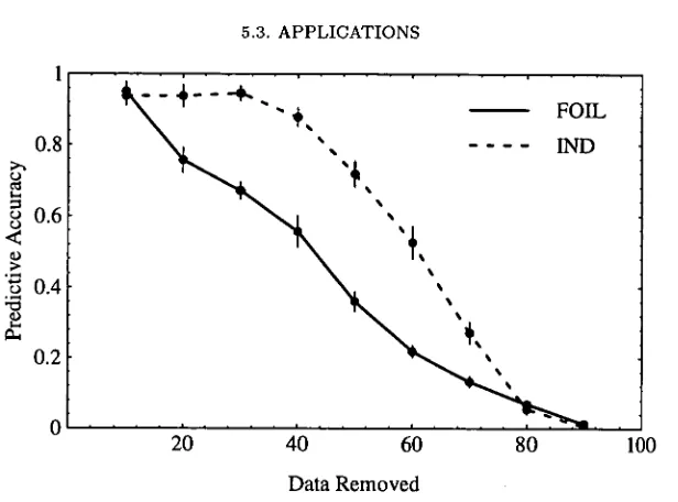
5.4 Predictive performance of FOIL and rewrite induction 85
6.1 Measure based on hypothesis testing 87
6.2 Posterior measure based on a uniform prior distribution 89 6.3 Posterior measure based on a binomial prior distribution 90
6.4 Measure based on predictive power 91
6.5 General predictive measure 92
6.6 Declining self-information of supporting observations 93
6.7 Declining entropy of observations 94
6.8 Growing knowledge in a blocks world 107 6.9 A blocks world with multiple theories 108
List of Tables
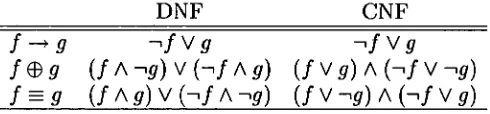
3.1 Disjunctive and conjunctive normal forms 35
3.2 Inference rules for KBC 40
3.3 Results of subproofs for Example 3.27 46
4.1 Dialogue with truth (based on Example 3.1) 60 4.2 Dialogue with side condition (based on Example 3.22) 60
4.3 Dialogue without answer 60
4.4 Dialogue with impossibility 61
4.5 Dialogue with impossibility (revisited) 61 4.6 Dialogue with hypothetical (based on Example 3.17) 62 4.7 Dialogue with local impossibility (based on Example 3.28) 63
4.8 Dialogue with contraction 64
4.9 Dialogue with a changing view 66
6.1 Maximally consistent sets for Figure 6.9(e) 108 6.2 Maximally consistent sets for Figure 6.9(f) 109 6.3 Maximally consistent sets for Figure 6.9(g) 109 6.4 Unique maximally consistent set for Figure 6.9(h) 110 6.5 Maximally consistent sets from D3 113 6.6 Maximally consistent sets from N i. 117
7.1 Dialogue with simple answers 123
LIST OF TABLES
7.2 Dialogue with crucial experiments
124
7.3 Dialogue with crucial experiments (continued) 125
Acknowledgments
I would like to deeply thank Desmond Fearnley-Sander for his guidance and patient supervision during this work. His great idealism and sense of purpose have been an inspiration throughout.
Simon Wotherspoon, Tim Stokes, arid La Monte Yarroll have been invaluable both in discussions of the material and in their friendship. I would also like to thank Kym Hill for his technical assistance, and all of the members of the Mathematics Department for its rich atmosphere. Finally, I give special thanks to my wife, Bronwyn, for her constant support.
CHAPTER 1
Introduction
Both automated reasoning and term rewriting have a rich history. However, much of the focus in automated reasoning has been on methods based on classical logic and logic programming systems. Although some applications of term rewriting have been considered, such as in [26], it still remains a small part of the field. In this work we seek to present a general and unified approach to automated reasoning through term rewriting.
Our broad aims are then two-fold. Firstly we give a thorough set of algo-rithms for reasoning by term rewriting. These include completion algoalgo-rithms for systems of equations and inequations, and an algorithm for generating function equations inductively from a ground rewrite system. The second aim is to use this concrete system of rewriting methods as a means of defin-ing and explordefin-ing standard notions of deductive and inductive reasondefin-ing. Of course these aims are intimately dependent on each other. The result will be a working prototype which is both motivated by and useful for rea-soning. With this in mind we will often talk about a reasoner, meaning simultaneously the idealized model of reasoning and the resulting concrete implementation.
We begin in Chapter 2 by giving the language in which we represent our knowledge and with which we reason. Term equations are a natural means of meeting these two needs. In order to concentrate on reasoning as much as term rewriting we adopt the simplest algebra of terms in which everything is ground (that is, variable-free), as given by Fearnley-Sander [15]. This language is still very expressive and also has a number of theoretical ad-vantages, such as the decidability of termination for a given rewrite system [12]
An important addition to the basic language of terms is the set constructor, a special instance of the potential entities described in [4]. The role of function terms can be quite limiting as confluence requires each function to have no more than one value. Sets provide a convenient method of handling multi-valued functions.
Chapter 3 looks at automated deductive proof techniques. The traditional method of deciding whether an equation is an equational consequence of a system E is to find a canonical rewrite system,
R,
for E and reduce both1. INTRODUCTION 2 sides of the equation with R. We call such a method proof by normalization and note that it is limited in a number of ways. It gives no procedure for generalizing to proving inequations from systems of equations and inequa-tions, and will also fail to prove a valid equation if the initial stage of finding the canonical system does not terminate.
We instead concentrate on proof by contradiction whereby we add the nega-tion of the equanega-tion to be proved to the system and seek a canonical form of the extended system. If in doing so we find that the system is inconsistent then we say that the equation is proved. This procedure is then immediately
semidecidable since every valid equation will eventually give such a contra-diction if the completion algorithm maintains its system in reduced form at each stage. We can also immediately prove inequations, their negations now being equations that get added to the system of hypotheses.
If the completion of the extended system terminates but does not find an inconsistency then we can interpret the result as side conditions, condi-tions which can be added to the original hypotheses to produce a theorem which can be proved. This gives the automated deductive reasoner a level of meta-reasoning, whereby it can not only prove a valid theorem but can also identify why it could not prove a non-theorem.
Related to the identification of side conditions is the process of solving a system of equations for an unknown. While we do not have variables in our term language, we can treat certain terms as being indeterminate in meaning. This gives a process for finding values for such unknowns which does not require any unification procedure.
The algorithm used for proof by contradiction processes single equations and inequations only. However, we extend the proof method to a full propo-sitional language in which the equations are the atoms. Reduction of the hypotheses and conclusion to disjunctive and conjunctive normal forms, re-spectively, generates a collection of subtheorems required to prove the origi-nal theorem. In Chapter 4 we show that this extension of the proof method to the propositional language gives a consequence relation, and hence forms the reasoning component of an AGM belief system [20].
1. INTRODUCTION 3 In particular, we give an algorithm which is proven to give a unique reduced form for equivalent systems of equations and inequations. This gives rise to a third deductive proof technique, dubbed proof by invariance, whereby a conclusion is a consequence of a system if the canonical forms of the system and the system augmented by the (non-negated) conclusion are the same. The automated proofs so far have all been of deductive theorems, but we can also automate the proof of inductive theorems, where the conclusion is an inductive consequence of the hypotheses. This is the induction of
mathe-matical induction, for which proof by consistency is a well known approach. We formalize it in our theory of term algebras and are able to characterize inductive theorems and the unambiguity property of Kapur and Musser [31] needed for proof by consistency to be valid.
A second kind of induction is that of scientific induction where we make observations and then conjecture new theorems based on the observations. We present an algorithm in Chapter 5 which generates function equations from a given rewrite system, the rewrite system capturing the observations made together with other general knowledge. We are then able give results which make concrete the relation between the mathematical induction and this scientific process.
Because of our simple term language we are able to quantify notions of belief using probability theory. We initial look at several probability measures of the strength of a single conjecture, based on statistical hypothesis testing and on the amount of information present in the conjecture. Later when looking at a system of conjectures, a theory, we extend these notions to quantify Popper's falsifiability measure of the strength of a theory [38]. We also look at qualitative information about belief, particularly the consis-tency of a belief system. In Chapter 4 we apply these ideas to systems based on declarative knowledge, where the reasoner is told information which it must then decide whether or not to believe in. We can use a close-minded model where any information that is inconsistent with already established beliefs is rejected, giving a monotonicity of belief. Alternatively, we can treat all declared knowledge as mutable, so if inconsistent information is given then we may instead reject earlier held beliefs.
When we move to inductive reasoning we must then make similar decisions about our inductively generated knowledge. In this case all of our knowledge is contingent on the observations from which it was conjectured and so if the total set of conjectures is inconsistent then we must find some subset to take as a working theory. Another kind of meta-reasoning arises here with the reasoner also being able to decide what is causing the inconsistency between possible theories. The result is that the reasoner can decide what
1. INTRODUCTION 4
CHAPTER 2
Preliminaries
2.1. Language
The language we will use is that of variable-free terms. The first section here defines this algebra in terms of a generating signature. In subsequent sections we introduce structural relations between certain terms in the lan-guage, capturing these relations as rewrite rules.
2.1.1. Algebraic Definition
A signature E is a pair (S,57 —s• x .5.) , where S is a non-empty set of sorts and Es* x s* is a family of sets, not necessarily disjoint, indexed by 5* x S*, where 5* is the set defined by
1. ground, sentence E S*;
2. If s E S then s E S*; 3. If s,tES*thensxtES*;
4. If s E S*,s ground, then {s} E S*.
An element f of E( is an operator of type (a, 7), and we say f has domain
a and codomain 7. If f has type (a, r), we will write f : a —> 7. If an operator f has type (ground, 7) we will also write f E T and say that f is a grounded term of type T.
We additionally require that each set E contains the identity operator
ia : a —4 a, that each set E,r) contains the empty set 0 : a —> T, and that
each 5T: —(a,ground) is a one-element set containing the erase operator !, : a —+ ground.
We also identify the sort {{a}} with the sort {a}, as expressed in the struc-tural rule S7 given in Section 2.3.3.
A signature E generates the term algebra TE. The terms of TE are defined and constructed by:
1. Each operator f E E(,,T) is a term of type a —4 T;
2. If f is a term of type a —> T then f is also a term of type {a} {7};
2.2. PREDICATES 6 3. If t1 , , tr,, are terms of type a al, , a
-
an then the tuple (ti,... ,tn) is a term of type a x • • • x an;
4. If t1 , , 4, are terms all of type a T then the set {t1,... ,tn} is a term of type a ---+ r;
5. If t is a term of type a T and f is a term of type T then the
application ft is a term of type a —* 11).
If f : T is a term with a not ground then we call f a E-function. If f is term arising from 1. then we call f a E-word.
2.1.2. Categorical Definition
For a given S-sorted signature E, we have an associated category CE with • objects S*,
• morphisms consisting of the operators in Es. x s,
• a function dom defined by dom(f) = a if the morphism f arose from an operator in
• a function cod defined by cod(f) = T if the morphism f arose from an operator in
• an identity morphism ia for each object a, corresponding to the identity operator i, E E(,,,), and
• composition o given by term application defined above.
Additionally the object ground is a terminal object for the category, with !, the unique morphism from a to ground.
The terms of our language are now generated by composition in this cate-gory, that is, by "following the arrows". This gives a simple pictorial way of describing a signature and the language it generates. We will usually use juxtaposition in place of o.
The category will have products if the signature contains any operators of arity greater than one. Much can be achieved though with only unary operators.
2.2. Predicates
In addition to the terminal object ground, each E also has the distinguished object sentence. An element of sentence is to be thought of as a truth value, while a morphism from a sort a to sentence is a predicate on a. We always have the two elements True, False E sentence.
We further extend our signature E, and the term algebra it generates, by introducing for each sort a the new morphism
2.2. PREDICATES 7
Consider the signature
= Alice, John E person, E
father : person —> person •
We can then represent the equality of the terms father Alice and John as the single term
=person (father Alice, John).
We can similarly define the new morphisms 0, and to represent inequa- tions and rules. We will usually write =,, 0,, and as infix operators. The a is also determined by the codomains of the equated terms (which naturally must be same) and so we will usually write =a as the polymorphic
Note that if f, g : r —> a then =, ( f, g) sentence so that dom(f = g)
is T. In particular, if dom(f = g) is ground, as in father Alice = John, we
call f = g a grounded equation.
For a given E we define the sets of >J-equations, EE, and E-rules, RE, by EE {S S I S, t E TE, S, t : 7}
RE = {S t I S7 t E TE, S, t : 7}.
For any E-equation e of the form s = t we define the negation of e to be s t. The set of E-inequations, –,EE, is the set of negations of all E-equations. We Write FE = U —ICE for the set of all E-equations and E-inequations. We will call a subset F C FE a E-system.
Note that we also have an empirical notion of equality, where we treat the terms as strings. In particular, for s,t E TE We write s t if s and t are identical (as strings), and s t if s and t are not identical.
To express conjunctions we introduce
and : sentence x sentence —> sentence
so that we may, for instance, form the term
and (father Alice =person John, male father =sentence True !).
We similarly define or, xor, implies, and not.
2.2.1. Entities
f
f, if dom (g) = ground; S3: f ! gf
if dom(g) 0 ground2.3. STRUCTURAL RULES 8
Alice, John, Paul E person. We call such declared words the E-entities of E. The products and sets of entities are also automatically entities.
The important point is that these entities are distinct. Having declared a collection of E-entities we implicitly require that any E-system F contains the inequation a 0 b for all E-entities a and b with a # b. Thus if we declare True and False to be E-entities then every E-system will contain True 0 False. We will usually declare ground words to be entities by writing them with an uppercase letter (reflecting the similarity with a proper noun). Any grounded word that is not declared to be a E-entity is called a indeterminate. Without Without the implicit entity inequations it is possible to have a consistent system with x = John, for example. Indeterminates thus serve the purpose of variables in the sense of solving equations, rather than in a unification process (see Section 3.7).
Indeterminates should always be ordered higher than entities. For example, the equation x = John oriented as x -4 John makes sense as a variable assignment whereas John x does not conform to our notion of entity. It is possible to view any grounded term as an indeterminate. The rule father Alice ---+ John in a sense assigns the value John to the indeterminate father Alice.
2.3. Structural Rules
The structural properties of our definitions so far can be captured using rewrite rules. Throughout our work we will assume that the rules given in the following sections are available for reducing a term to normal form.
2.3.1. Category without Products
The only rules we require for a category without products are those for the identity and erase morphisms. These are given in [28] and are as follows:
Si: i f f S2:
f
i —> f2.3.2. Category with Products
2.3. STRUCTURAL RULES 9 The inclusion of projection operators can also help model certain reasoning tasks, but their use is unnecessary for our purposes.
2.3.3. Sets
A potential entity is an algebraic construction that models a case statement and their inclusion in rewriting systems greatly increases the reasoning that can be performed. For example, the potential entity
cas e((a, f), (0,g), (6,h))
is potentially f, g, or h, depending on the value of the boolean conditions a, 0, and S. These general constructions, originating in [15], have a rich algebraic structure [4]. However, a restricted form of them motivates a construction for sets of terms.
Consider the example of the function aunt which models the function that returns the aunt of a person. Since a person may have more than one aunt, this function is multi-valued and hence cannot be directly captured by a confluent rewrite system. Potential entities in which the boolean conditions are completely indeterminate may be viewed as sets.
For example, as a potential entity we could write the function aunt as aunt = case((a, sister father), (0, sister mother))
or, using set notation instead, as
aunt = {sister father, sister mother}.
The elements of the set must all be of the same type o- —> T, giving a set
of type o- {r}. The structural rules for sets are the same as those for potential entities [4], suppressing the boolean conditions:
S5: I {gi, •••, gn} {fgi, •••, S6: fn} g {fig, fng}
S7: {• • • , {gi, .••7gM}7 • • } {• • • 7 gll •••7 gM7 • • • }
S8: {f, f7 g17 •••I gn} {f, gi, •••7gn}
S9: ({fi, , fn}, {(L, g), • • • , (fn, 9)1 S10: (f, {gi,... , gm}) , (f, gm)}
S5 and S6 define the relationship between f : a —4 r and f : {a} —› The next four involve alterations to the boolean conditions in the case construction, but these are not explicitly of interest when looking at sets. Our sets are commutative since the order of terms in potential entities is irrelevant.
2.3. STRUCTURAL RULES 10 ought to be type-preserving, which is not the case if we replace {f} by
f.
Related to this is an ambiguity in the associated equational reasoning. If
F =
{aunt Alice = {Jenny}, aunt Alice = {Kelly}},then we have {Jenny} = aunt Alice = {Kelly}, indicating that
F
is inconsis-tent. If we allow {f}= f
then we also haveaunt Alice = {aunt Alice} = {aunt Alice, aunt Alice}
= {{Jenny}, {Kelly}} = {Jenny, Kelly},
giving a second equational meaning of
F.
Hence we exclude {f} =f
so that if Alice indeed has two aunts then we must give the single equation aunt Alice = {Jenny, Kelly}. The implications of this are seen again in Ex-ample 3.33. It is possible for an implementation to invoke a preprocessor to convertF
intoF' =
{aunt Alice = {Jenny, Kelly}}. A practical rea-soner should be able to learn aunt Alice = {Jenny} and the later learn aunt Alice = {Kelly} without giving inconsistency, particularly under the assumption that its data is noiseless. However, this is a meta-reasoning and not part of our equational theory.Working with the boolean conditions of potential entities requires binary boolean operators, and hence products. Another advantage of the above structural rules is that by not manipulating the conditions, we can work with sets without the necessary presence of products.
EXAMPLE 2.1 (Set reduction). As an example of the structural rules S5-S8, consider the signature
Alice, John, Jill, Jenny, Kelly, Mary E person,
= father : person person, E
sister, aunt : person --* {person}, female : person --+ sentence
and rewrite system
/aunt —> sister {father, mother},
father Alice John, mother Alice + Jill, ----
R =
sister John {Jenny}, sister Jill {Kelly, Mary}, . female Jenny --- True, female Kelly —> True,female Mary True
2.3. STRUCTURAL RULES 11 Finding the value of female aunt Alice makes use of all of the given rules not involving products:
female aunt Alice
female sister {father, mother}Alice -+S6 female sister {father Alice, mother Alice}
female sister {John, Jill} -->S5 female {sister John, sister Jill}
female {{Jenny}, {Kelly, Mary}}
- 4 S7 female {Jenny, Kelly, Mary}
- + S5 {female Jenny, female Kelly, female Mary} -1=t {True, True, True}
-+ S8 {True}
In E the type of female is person sentence, but the construction of TE in- cluded the term female : {person} {sentence}. This is the morphism used in the term female aunt Alice. The change can be made explicitly through type inference, or implicitly, as above, through the rules S5 and S6. 0 We can view equality as a binary operator so that we may write, for example, a term
= (aunt, sister {father, mother}).
This then involves a product of sets, and so is structurally reduced to the set of equations
{aunt = sister father, aunt = sister mother}.
Equations involving internal set constructors thus express (non-exclusive) disjunction, as opposed to the standard sets of equations, our equational systems, which we view as conjunctions.
However, this structurally reduced form is less amenable to rewriting than that used in the R of Example 2.1. We will usually view equality and rewrite as being external to TE, maintaining = and at the head of term expressions.
2.3.4. Term Orderings
Let S be the set of structural rules Si-S10. A term s is in structural normal
form if s cannot be reduced by S. A term s is the structural normal form
of a term t if t s and s is in structural normal form.
2.3. STRUCTURAL RULES 12 For example,
6(father Alice) = 2, 6(and(male Alice, True)) = 2, b({Alice, Lucia}) = 1.
Since sets distribute to both the right and the left, any term involving a set will have length 1.
DEFINITION 2.2. Given an ordering > on the words of E, we extend > to TE by giving an ordering on terms s,t E TE in structural normal form.
• If 6(s) 0 6(t) then s > t if and only if 6(s) > 6(t); • if 6(s) = 6(0 then
— if s = (s1,... , sn),t = (si,. ,sn) and k > 0 is the first integer such that sk tk then s > t if and only if sk > tk;
if s = {si, , s,}, t = {si, , sm} , where the si and t2 are or- dered by >, then
* if n m then s> t if and only if 11> 771;
* otherwise if k > 0 is the first integer such that sk tk then
s > t if and only if sk > tk;
— otherwise if s = si • • • sn , t = t1 • • tn, and k > 0 is the first integer such that sk tk then s > t if and only if sk > tk;
Thus for example
father Alice > John,
and(male Alice, True) > and (True, male Alice), {father Alice, Paul} > {John, Paul}.
CHAPTER 3
Proof Methods
In this chapter we are primarily interested in developing a complete proof method for deductive theorems over the propositional language with equa-tions as atoms and connectives V, A,
ej.
We find that the most amenable method is proof by contradiction, though an associated process, proof by invariance, will also play an important role. Along the way we will also examine the proof of inductive theorems, look at how non-theorems can be extended to give theorems, and finally consider how we might solve systems of equations in a variable-free language.3.1. Equational Proof
DEFINITION 3.1. Let
F
be a E-system. We define the relation =F on TEas follows:
Axiom: If (s = t) E
F
then S =F t. Reflexivity: S =F S for all s E T. Symmetry: If S =F t then t =F S.Transitivity: If S =F t and t =F U then S =F U.
Application: If S =F t then SU =F tU for all u E TE with cod(u) = dom(t). Product: If S =F t then (... , s,...) =F (• • • ,t, • • •)•
Set: If S =F t then {.. • ,s, • • • =F {• • • ,t, • • •}•
Structure: If s t by the structural rules Si - S10 then S =F t.
If S =F t then we write
F =
(s = t) and say that s = t is a consequence ofF.
DEFINITION 3.2. If S =F t for some (s t)
E F
thenF
is an inconsistentE-system, and we write
F
H
I. OtherwiseF
is said to be a consistentsystem.
A rewrite system
R
over TE is a subset of the rewrite rules R.E. The appli-cation of a rule(1
—>
r) ER
on a term s involves replacing an occurrence of1
in s (if any) with r. If the resulting term is t we say that s rewrites to t3.2. PROVING EQUATIONS 14 If s —*R t and t cannot be rewritten by R then we say that t is an R-normal
form of s. If there is some u such that s u and t —>*R u then we write
S 4-* t.
If there is no infinite rewriting S S1 • • • then we say that R is
terminating. Termination is a decidable property for our ground language
TE [12].
3.2. Proving Equations
Our first goal is to outline three methods for proving that a specific equation is the logical consequence of a set of equations. These methods will then be used as the basis for the more general problem of proving an equation or inequation to be a consequence of a system of equations and inequations. The first method, proof by normalization, is a standard equational proof technique. Relying on the soundness and completeness of the Knuth-Bendix procedure, we prove an equational conclusion by normalizing it with respect to a canonical rewrite system generated from the equational hypotheses. This method gives no generalization to systems involving inequations, and will fail to prove a valid equation if the canonical system is unbounded. This lack of semidecidability has been addressed in [13], but here we avoid it by introducing a second method, proof by contradiction. For such a proof we augment the hypotheses with the negated conclusion and then reduce the resulting system. This requires an extension to the Knuth-Bendix procedure to process inequations.
This extended procedure is sufficient to prove anything by contradiction that could be proved by normalization, in addition to allowing proof from hypotheses involving inequations. However, for equations alone we also have the strong result that two systems are equivalent if and only if their canonical forms are identical. This gives rise to a third technique, proof by invariance. Our final task is to obtain a canonical form algorithm for systems with inequations which has this same property.
3.2.1. Proof by Normalization
The standard rewrite method for determining whether F f is to find a canonical set of rewrite rules R for F and apply those rules to each side of the equation. Such a canonical set is generated by the Knuth-Bendix completion procedure ( [32], [29], [13], [7]). Since the Knuth-Bendix procedure is sound and complete [27], both sides have the same normal form if and only if
F H f. We thus call this rewrite-based method proof by normalization.
Define
3.2. PROVING EQUATIONS 15 The Knuth-Bendix algorithm is presented below.
3.2.2. Basic Knuth-Bendix Procedure
It will be useful to view completion as a function which takes a set of equa-tions and inequaequa-tions and returns a set of rewrite rules and inequaequa-tions. Thus we define KB : P(CE U P(RE U –,EE) to be the Knuth-Bendix algorithm. For a system
F
C FE, the algorithm begins in the initial state (E0 , Uo ,0),
whereE
0
=F n EE
and Uo =F
n The following inference rules (see [13] and [26] for these with equations alone) are then repeatedly applied in order:Delete (E U {s = s} , U,
Compose (E,U, RU {s t})
Simplify (E U{s = t} , U, R)
Orient (E U {s = t},U, R)
Collapse (E ,U, RU {s —› t})
Deduce (E,U, R)
(E, U, R)
(E,U, RU u})
u{s= u},U,
(E,U, Ru Is t})
(E u fu = t} ,U, R)
(E u = tl,U, R)
if t u
if t -+R u if
s
>t
if S ->R u ifS
--+Rt If this process terminates inN
steps with final state(EN, UN, RN)
then we say that KB(F) =UN
URN. (EN
will always be empty if the procedure terminates). If the process does not terminate then we say that the canonical system forF
isunbounded.
It is also possible for the process to fail if at some stage the rewrite rule sys-tem Rk is non-terminating. This cannot happen when using a total-degree ordering but may happen for other orderings (see Example 3.2). Dauchet and Tison [12] give an algorithm for deciding the termination of a rewrite system, and this can be used if necessary to check for failure. If the proce-dure does not fail in this way and terminates we say it is
successful.
Note that the inequations inF
are unaffected by the KB procedure. That is U0 =UN,
or alternativelyKB(F) = KB(E0) U Uo.
We will later extend the list of inference rules given above to process inequa-tions as well.
EXAMPLE 3.1 (Normalization proof). The majority of examples in this chap-ter use a toy world described by the signature
John, Jill, Alice, Lucia, George, Bob, Paul E person, father, mother, husband, wife,
sister, fatherinlaw : person --+ person, male : person sentence
3.2. PROVING EQUATIONS 16
Bob Betty
Jenny John
George 1 Kate
I
I
iJill Kelly Mary --1— Peter
Alice Lucia Paul
FIGURE 3.1. Motivating family tree
Consider the theorem
F =
{father sister = father, sister Alice = Lucia},f =
(father Alice = father Lucia).In proving this by normalization we first apply KB to
F
to obtain the rewrite systemR =
father sister --+ father, sister Alice Lucia, father Alice —+ father LuciaThe normal form of the left-hand side of
f
with respect toR
is father Lucia, as is that of the right-hand side, thus proving the theorem. 03.2.3. Uniqueness of Canonical Rewrite Systems
DEFINITION 3.3. A rewrite system
R
isconvergent
for a set of equationsF
ifR
presents the same theory as doesF,
i.e. ifs t
if and only ifS =F
t. DEFINITION 3.4. A rewrite systemR
isreduced
if for all(s t)
ER, t
is in normal form with respect toR
ands
is in normal form with respect toR\(s t).
DEFINITION 3.5. A reduced and convergent rewrite system is said to be
canonical.
Huet [27] has shown that the output of KB(F) is a canonical system for
F.
If we do not have a total ordering on our terms then an equational theory may have more than once canonical rewrite system, as seen in [13]. If we allowed variables in the algebra then obtaining a total ordering may be difficult, and even if we had one the best we can say is that the canonical rewrite systems will be isomorphic [14]. By working with our ground algebra we can always obtain a total ordering,as
given in Section 2.3.4, and furthermore we have the following strong result:3.2. PROVING EQUATIONS 17 PROOF. Let RI, R2 be two canonical rewrite systems for F, with R1 0 B2. Consider any (1 —> r) E R2 \ Ri. Since B2 is convergent we have that /
=F
r, so we must have a rewrite proof of 1 =F r from the rules in R1 , as R1 is also convergent for F.Suppose r is not a normal form under R 1 . Then we have 1 s <—*Ri r, for some s, with 1 > r > s. Again, since R 1 is convergent for F, we have r =F S, so in R2 we must have r t 4—*R2 s, for some t, with r> s > t. This gives / --q?2 t, with r > t, which contradicts R2 being reduced.
If r is already a normal form under R 1 then we must have 1 s, since 1 # r, with 1 > s. Thus 1 =F S so under R2 we have 1 t 4—*R2 s, for some t, with 1 > s > t. This now gives / --4*R2 t, with 1 > t, which again contradicts R2 being reduced.
Either case gives a contradiction, so we must have R 1 = B2.
This theorem is motivated by the corresponding result for reduced Grobner bases [9]. Polynomial algebras share the lack of variables with our ground term algebras, making the completion procedures for each very similar. This is particularly apparent when looking at the non-commutative polynomials of [34].
The uniqueness theorem gives rise to several other results which are useful in formulating proof strategies.
COROLLARY 3.1. For a given input F and fixed term ordering, the output of KB is independent of the order in which the equations in F are processed.
PROOF. As mentioned above, the output of KB is a canonical rewrite sys- tem for F. Theorem 3.1 gives that this is then necessarily independent of
equation ordering. 0
This trivial result is not so trivial when extending KB to process inequa-tions. We include it here for comparison with the development of KBC in Section 3.4.4.
In our applications we will almost exclusively use a total degree ordering on our terms (see Section 2.3.4). This guarantees that at every stage of the Knuth-Bendix process the set of rewrite rules R is terminating. How-ever, sometimes a lexicographic ordering is more appropriate for a particular problem, as in the following example:
EXAMPLE 3.2 (Lexicographic ordering). Consider a model of the group of square symmetries with two generators h and r. We view these as a reflection and a rotation which map the corner points of a square onto its corner points, and so give a signature
3.2. PROVING EQUATIONS 18 (This model is presented in more detail in Section 6.4.2). Three equations are sufficient to define the behaviour of the two functions, giving
FD ={ hh=i,rrrr=i, rh=hrrr 1.
With a total-degree ordering on terms, if r > h we obtain the canonical system
R1 ={ hh—>i,rhr—>h,rrr—hrh,rrh--hrr while if h > r then we get the larger system
hh--+i,rrrr-->i,hrh-4rrr, R2 = 1 hrr—*rrh,rhr—>h,rrrh—dir
The real aim of finding a canonical system for FD is to be able to deter-mine which sequences of rotations and reflections are equivalent by finding normal forms for them. The normal forms produced by R 1 and R2 can be rather strange in relation to the original model. The natural and pragmatic normal form would instead be a sequence of reflections followed by a series of rotations, and this is what we obtain with a lexicographic ordering and r> h:
R3 = hh—+i,rrrr--i,rh—hrrr 1.
Even though the last rule increases the length of a term, we know it is terminating because it moves an h to the left at every step.
Unfortunately, lexicographic ordering is not perfect for this example, since if we chose Ii > r then during KB Deduce would produce a new equation rh r=h which is oriented as h r h r and gives a non-terminating system. Hence for this ordering the KB procedure fails. Since this can be detected, as in [14] , some form of backtracking may be useful. 0
Given then that we may be interested in using lexicographic orderings, we rephrase the previous corollary as:
COROLLARY 3.2. For a given input F and fixed term ordering, if KB
suc-ceeds then the output KB(F) is unique.
The last result we are interested in gives an important relationship between equivalent equational systems and KB. Constructing an algorithm for sys-tems with inequations with the same relationship will be our focus in Sec-tion 3.4.4.
DEFINITION 3.6. If F1 = e if and only if F2 j= e then F1 and F2 are said to be equivalent systems of equations.
3.2. PROVING EQUATIONS 19 Th
PROOF. If F1 and F2 are equivalent then S =F1 t if and only if S =F2 t. We
can modify the proof of Theorem 3.1, using F 1 , F2 for RI, R2, to show that KB(F1 ) = KB(F2).
The converse holds by the soundness of KB. 0
This corollary justifies proof by invariance, to be discussed in the following section. Also, since F and R = KB(F) are equivalent, it gives the additional result:
COROLLARY 3.4. For a set of equations F and an equation f,
KB(F U f) = KB(KB(F) U f).
3.2.4. Proof by Invariance
A second method of determining whether f E F is entailed by F C e is to apply the Knuth-Bendix algorithm KB to both the sets F and F U f. If f is indeed implied by F then F and FU f are equivalent, so by Corollary 3.3 the results of KB will be the same.
We write
F kKB f if KB(F) = KB(F U f
and define FKB={fETIFkKBf}. PROPOSITION 3.1. FKB, = FKB•
PROOF. If f E FKB„, then by the soundness and completeness of the Knuth-Bendix procedure we have that F
H f.
Thus the two sets of equations F andFU f are equivalent, and hence by Corollary 3.3 we have KB(F) = KB(FUf),
so that f E FKB.
Conversely, if KB(F) = KB(F U f) then at some stage in the right-hand application of KB the inference rule Delete must have been used to remove
f. That is the equations of F must be used to reduce both sides of f to the
same term, so that f E FKB,. 0
EXAMPLE 3.3 (Invariance proof). Consider again the theorem given in Ex-ample 3.1. The canonical system for the hypotheses F is the given
R = father sister father, sister Alice Lucia,
father Alice father Lucia
Depending on the order in which KB processes the equations, when finding the canonical system for FU f either f will be reduced to a tautology by the
3.2. PROVING EQUATIONS 20 Note that from the earlier identity KB(F) = KB(E 0) U Uo we can never use
KB to prove that an inequation is the consequence of a system.
3.2.5. Proof by Contradiction
An alternative method of proving an equation to be the consequence of a sys-tem is proof by
contradiction.
We will show that this method can prove any equation that could be proved by normalization or invariance. Additionally proof of inequations from a system of equations and inequations is imme-diately possible, information about non-theorems can be obtained from the result of the contradiction method, and a contradiction proof incorporates a useful semidecidability (as seen in Example 3.5).To prove the theorem
F =f
by contradiction we find the canonical form of the systemF U
If it includes a contradiction then the theorem is true, otherwise it is false.To find contradictions in the system we need to extend the basic Knuth-Bendix procedure so that inequations are processed. For the system
F =
E
0
U U0 , this can simply be done by completing E0 alone and reducing the inequations in U0 with the result. However, this separation is somewhat artificial in that we would like to viewF
as a complete theory in itself. This is highlighted by a case where KB(E0) is unbounded butE
0
U Uo is inconsistent. Contradiction then gives a semidecidable proof procedure, as illustrated in Example 3.5.To define a proof by contradiction method we extend the set of inference rules for KB to obtain a new procedure, Knuth-Bendix with
inequations,
or KBI, which we can apply to the whole theoryF.
The two rules needed are the following:Contradiction (E U {s s} , 1
SimplifyU (E U
{st}, R) = (E U u} , R)
ift
These two inference rules generate no additional equations or inequations and so do not effect the termination of the Knuth-Bendix procedure. Specifi-cally, if KB had terminated then the equation set given as input would have been reduced to the empty set. Unless a contradiction is obtained, the equation set in KBI will also reduce to the empty set. The number of in-equations will be the same, but each will be in reduced form with respect to the generated rewrite rules.
3.2. PROVING EQUATIONS 21 Since the completion of the equations in a system
F
is unaffected by the inequations inF,
we have the following simple result:LEMMA 3.1.
For F C .F with K.131(F) 0 1,
KBI(F)
n
=KB(F
n
e).
With KBI : P(T) P(R, U —,£) we can introduce the corresponding notion of entailment. We define
Hum-,
byF
k
KBE
,
f
if KBI(F U=
and again putFlum-, = {f E F
F
Hum-,
f }.
PROPOSITION 3.2.FKB =
PROOF.
Suppose
(1 =
r) E FKB so that KB(FU(1 = r)) =
KB(F). Then at some stage of KB the inference ruleDelete
must be invoked, so that(1 =
r) must reduce to give an equation(s = s).
But then in the application of KBI the corresponding inequation(1
r) will produce the inequation(s s),
a contradiction, so that KBI(F U(1 0 r)) = 1,
giving(1 =
EThe proof of the converse is similar.
This result shows that we can prove anything that could be proved using KB alone. Additionally we are now able to prove theorems with hypotheses or conclusion in
,
as discussed in Section 3.4.1.We can now be more precise about the notions of
theorem
andproof.
ForF C .F
andf
E .7. we call the pair(F, f)
apossible theorem.
IfF Hum
-,
I
then we call(F, f)
atheorem
and writeF = f.
If KBI(F Uf) 1
we call(F, f)
anon
-theorem
and writeF f.
We will talk aboutproving
a possible theorem(F, f),
the empirical act of computing KBI(F U --if), and say that(F, f)
isproved
if we find thatF = f.
EXAMPLE 3.4 (Contradiction proof). Returning again to Example 3.1, we want to prove the possible theorem
(F, f),
whereF =
{father sister = father, sister Alice = Lucia},f =
(father Alice = father Lucia).We thus apply KBI to the augmented system
father sister = father, sister Alice = Lucia,
F U f =
father Alice 0 father Lucia
3.2. PROVING EQUATIONS 22 EXAMPLE 3.5 (Unbounded hypotheses). Consider the set of equations
F
= { father Jill = George,fatherinlaw father = father mother J'
from which we would like to prove the conclusion
father mother Jill = fatherinlaw George.
A normalization proof requires a canonical system for F but KB(F) is un-bounded, containing the rules
father mother?' Jill -4 fatherinlawk George
for all k > 1. Hence the first part of the normalization proof cannot succeed. For a contradiction proof the negated conclusion leads to I with the first rule generated, thus terminating KBI and proving the theorem. 0
In an implementation of KBI we must naturally try to detect an unbounded completion process and terminate the procedure. Since the rewrite system is maintained in reduced form one way of doing this is to set an arbitrary bound on the length of terms that can be generated, declaring a system to be unbounded if we ever produce a new rule involving a term of length greater than this bound. If we abort in this way as part of a proof by contradiction then we will assume that we have a non-theorem.
EXAMPLE 3.6 (Non-theorem). Consider now
F = {father sister = father, sister Alice = Lucia},
f = (father Alice = John).
Applying KBI to F U -i f , with Alice > Lucia, gives
{
father sister father, sister Alice —> Lucia,
father Alice —> father Lucia, father Lucia
0
John •Thus F and f do not constitute a theorem since a contradiction was not found. However, the result of KBI can be used to determine what conditions need to be added to the hypotheses F to give a theorem. This process is considered in Section 3.5. 0
Working with a variable-free algebra means we have a trivial semantics for our systems, reflected in the simple definition of consistency (Definition 3.2). This allows the following important result, giving a test for consistency. LEMMA 3.2. F C .7' is consistent if and only if KBI(F) 0 I.
PROOF. Let E = F fl e, the equations in F. By Lemma 3.1 the rules, R, generated for E by KBI are a canonical system for E. Thus if F is not consistent then by the completeness of R there is a rewrite reduction of some (s E F to a contradiction, so that KBI(F) = I. Similarly, if KBI(F) returns I then by the soundness of R there is an equational proof
3.2. PROVING EQUATIONS 23
3.2.6. Proving Compound Sentences - Conjunction and Disjunc-tion
So far we have only looked at proving single equations, but the process can be extended to general sentences. The two simplest cases are conclusions involving the external connectives of conjunction (A) and disjunction (V). Firstly, to prove a possible theorem
(F,
h
A • • A fn) we must try provingeach
(F, A), ,(F, L
i
)
in turn, obtaining a theorem only if each subproof was successful (i.e. finding KBI(F U-ifj)
= I for eachj).
EXAMPLE 3.7 (Conjunctive conclusion). Consider the possible theorem with
F
=
male father = True !, father sister = father,sister Alice = Lucia, father Lucia = John
f =
(male John = True) A (father Alice = John).We find KBI(F U {male John 0 True}) = I and KBI(F U {father Alice 0 John}) = I, so that
F = f.
The case where the conclusion involves a disjunction, and indeed when it is any compound sentence in general, can be handled in a similar manner. A proof is attempted for each atomic sentence and then the results are com-bined to determine whether the whole compound sentence is a consequence of the hypotheses. For instance, to prove a possible theorem
(F, A
V • • • V fn )we must prove at least one of
(F, ,(F,
Li), requiring possibly n sep-arate applications of KBI.However, for disjunction we have an alternative approach which allows proof in just one step by noting that -, (fi V• • •Vfn ) is equivalent to (-ifi A • • •A--ifra).
Thus the negation of our conclusion is simply a conjunction of inequations, a
set
of inequations in the same way the set of hypotheses represents a conjunction. We can then apply KBI toF
u , —ifn
}
to determine whether(F, 1
1
V • • • VL
i
)
is a theorem.EXAMPLE 3.8 (Disjunctive conclusion). To prove the possible theorem with
F
=
father Lucia = John male father = True !, father sister = father,f =
(male John = True) V (father Alice = John). we apply KBI toF
U {male John0
True, father Alice 0 John}.A contradiction is obtained since the hypotheses reduce male John to True, giving
F = f.
3.3. PROVING INDUCTIVE THEOREMS 24
With this simple method for handling disjunctions we can work with any conclusion by expressing it in conjunctive normal form.
3.3. Proving Inductive Theorems
We begin this section with an example of a theorem that none of the pre-ceding methods can prove.
EXAMPLE 3.9 (Non-deductive theorem). Consider the signature = True, False E sentence,
E
not : sentence sentence
and the possible theorem with
F = {not False = True, not True = False},
f = (not not = i).
The reason that we might think of (F, f) as a theorem is that we have com- plete information about the behaviour of not and know that the conclusion holds for all entities in its domain. Yet F has the simple canonical system
R = {not False True, not True False},
which clearly cannot reduce —if to a contradiction. Hence F f.
The theorems we have looked at so far and have proved have all been de-ductive in nature. Our methods fail on this example as it is an inductive theorem. We will look extensively at the generation of such theorems in Chapter 5, but for now we give some definitions which motivate a corre-sponding proof method.
3.3.1. Strong Completeness
Let .F = e U —.6., the set of all equations and inequations between terms in TE. So far we have only defined s =E t for equations E; for F C .7* we write
S =F t if s =Fne t.
DEFINITION 3.7. Let FCY. A rewrite system R is weakly complete for F if whenever s =F t then s
This is the sense in which the result of Knuth-Bendix completion is com-plete, and (along with soundness) is the justification of our deductive proof methods. However, an alternative notion of completeness can be given in terms of consistency (see, for example, [6] and [30]).
3.3. PROVING INDUCTIVE THEOREMS 25
Hence if we have a strongly complete system then Lemma 3.2 gives a straight-forward procedure for deciding whether a particular equation is a theorem of that system or not. This is the technique of proof by
consistency,
also known as "inductionless induction" because it allows the proof of inductive theorems without the use of standard structural induction [23], [31]. To apply proof by consistency we need first to define more precisely what we mean by a theorem and then how we may characterize strongly complete systems. The following discussion develops the ideas in [31] for our proof system.DEFINITION 3.9. For
F
C F ande
EE,
if KBI(F U= 1
then we calle
adeductive theorem
ofF
and write (as before)F = e.
All of the theorems we have proved in previous sections have been deductive theorems, while the theorem of Example 3.9 was not. We write DF for the set of all deductive theorems of
F.
Note that ifF
is inconsistent then DF= E.
We say that e EE
isconsistent with F
ifF U e
is consistent, and write CF for the set of all equations that are consistent withF.
DEFINITION 3.10.
C
CE
is aconsistent theory
ofF
ifC
is consistent and VF CC
(and henceF
C C). C is amaximally consistent theory
if it is a consistent theory ofF
and there is noe E
such thatC
U e is consistent.Thus each consistent theory
C
ofF
satisfies DFC
CC
CF. The following lemma shows that DF is itself a consistent theory forF
and is thus the smallest consistent theory.LEMMA 3.3.
If F
C.F is consistent then
DFis
aconsistent theory for F.
PROOF. Since
F
is consistent, KBI(F) I. 'LetE=FnE
so thatR
= KBI(F)n7Z = KB(E).
SinceE = f
for eachf
E DF, we can perform a series of proofs by invariance to find that KB(E U VF)=
R.
ButF
is consistent so we knowR
does not reduce any inequation inF
to a contradiction, andhence DF is a consistent theory. Ei
Furthermore, we can similarly show that if
e
EE
is consistent withF
then it is also consistent with DF.EXAMPLE 3.10 (Unique maximal theories). For the
F
of Example 3.9, the deductive theorems ofF
areDF
=
{not2i False = not2i False, not2i False = not2i+1 True}, i,i>owhere we write not° for i. The set
3.3. PROVING INDUCTIVE THEOREMS 26 is a consistent theory for F while
=
DFU {not2i = not2i, not2i+ 1 = not23+1 } i,j>ois a maximally consistent theory for F. It is straightforward to see that CI is actually unique as a maximal theory. 0
EXAMPLE 3.11 (Multiple maximal theories). Consider a smaller system F' = {not False = True},
with deductive theorems
DFI
=
{noti False = not i-1 True}.i>1 This time both
=
DF, U {not not = i} and C2 = DF,U
{not not = not}are consistent theories for F but Ci U C2 is not consistent, since we have False =c, not not False =c,2 not False =F True.
Thus we cannot have a single maximally consistent theory for F since both C1 and C2 can be extended to a maximal theory. Indeed we find that
=
DF, U {not 2i = not 2i, not2i4-1 = not2j+1} i,j>oand C = DFI U {not 2i = not 2i+ 1 } i,i>o
are both maximally consistent theories for F. 0
DEFINITION 3.11. f E E is a theorem of F c .F if it is in the intersection of all maximally consistent theories of F.
We use TF to denote the set of all theorems of F. Since DF is a subset of all consistent theories, all deductive theorems are immediately theorems of
F.
LEMMA 3.4. If F c .F has a unique maximally consistent theory C then
C = CF. Conversely, if there is a consistent theory C such that C = CF
then C is maximal and unique.
3.3. PROVING INDUCTIVE THEOREMS 27 By the definition of a theorem, if an F has a unique maximally consistent theory C then the theorems of F are exactly the elements of C. We follow [31] and call such a system unambiguous. Conversely, if the theorems of
F are exactly the elements of some maximally consistent theory C, then C
must be unique. Lemma 3.4 then gives the important result:
THEOREM 3.2 (Strong Completeness). F is unambiguous if and only if
TF =CF7
that is, if and only if the theorems of F are exactly the equations that are consistent with F.
This statement is equivalent to saying that if F is unambiguous then CF is the only consistent theory for F.
3.3.2. Inductive Theorems
The equations we have called theorems of F are exactly those that must hold in any maximal and consistent theory for F. That is, if f is a theorem of F then in any consistent model where the equations and inequations in F hold, so must f. If f is a deductive theorem then we can indeed prove this relationship, using proof by contradiction. The remaining, non-deductive, theorems will be called inductive theorems of F.
DEFINITION 3.12. For F C .7' if e E E is a theorem of F and e DF then e is an inductive theorem of F.
The discussion so far has been quite general. In this section and the next we make more precise statements about the nature of inductive theorems and unambiguous systems.
DEFINITION 3.13. A sort a in a signature E is entity rich if there are at least two distinct E-entities a, b E a. A signature E is entity rich if each sort in E is entity rich.
We will assume in the following two sections that we have an entity rich signature. Without it most of the ideas and proofs become trivial. If f :
a —* 7 and 7 has only a single entity b, then any maximal theory must have fa = b and so ambiguity cannot arise.
For our language of a term algebra we can obtain the following characteri-zation of inductive theorems.
THEOREM 3.3. If the only inequations in F C .T are entity inequations and
e E E is an inductive theorem of F, then dom(e) 0 ground.
![FIGURE 5.2. Visual data for classification (from [3])](https://thumb-us.123doks.com/thumbv2/123dok_us/8469287.339950/97.565.158.407.84.314/figure-visual-data-for-classification-from.webp)
![FIGURE 5.3. Two isomorphic family trees (from [25])](https://thumb-us.123doks.com/thumbv2/123dok_us/8469287.339950/99.562.107.429.113.277/figure-isomorphic-family-trees.webp)