www.earth-syst-sci-data.net/9/193/2017/ doi:10.5194/essd-9-193-2017
© Author(s) 2017. CC Attribution 3.0 License.
KRILLBASE: a circumpolar database of Antarctic krill
and salp numerical densities, 1926–2016
Angus Atkinson1, Simeon L. Hill2, Evgeny A. Pakhomov3,4, Volker Siegel5, Ricardo Anadon6, Sanae Chiba7, Kendra L. Daly8, Rod Downie9, Sophie Fielding2, Peter Fretwell2, Laura Gerrish2,
Graham W. Hosie10, Mark J. Jessopp11, So Kawaguchi12, Bjørn A. Krafft13, Valerie Loeb14, Jun Nishikawa15, Helen J. Peat2, Christian S. Reiss16, Robin M. Ross17, Langdon B. Quetin17, Katrin Schmidt10, Deborah K. Steinberg18, Roshni C. Subramaniam19, Geraint A. Tarling2, and
Peter Ward2
1Plymouth Marine Laboratory, Prospect Place, The Hoe, Plymouth, Pl13DH, UK 2British Antarctic Survey, High Cross, Madingley Road, Cambridge, CB3 OET, UK 3Department of Earth, Ocean and Atmospheric Sciences, University of British Columbia,
2207-2020 Main Mall, Vancouver, BC, V6T 1Z4, Canada
4Institute for the Oceans and Fisheries (IOF), AERL, 231-2202 Main Mall,
University of British Columbia, Vancouver, BC, V6T 1Z4, Canada 5Thünen Institute of Sea Fisheries, Palmaille 9, 22767 Hamburg, Germany
6Department Biology of Organisms and Systems, University of Oviedo,
C/ Catedrático Rodrigo Uría s/n, 33071 Oviedo, Asturias, Spain 7JAMSTEC, 3173-25 Showamachi, Kanazawaku, Yokohama 2360001, Japan 8College of Marine Science, University of South Florida, St. Petersburg, FL 33701, USA
9World Wildlife Fund, The Living Planet Centre, Rufford House, Brewery Road,
Woking, Surrey, GU214LL, UK
10Sir Alister Hardy Foundation for Ocean Sciences, The Laboratory, Citadel Hill, Plymouth, PL1 2PB, UK 11MaREI Centre, Environmental Research Institute, University College Cork, Haulbowline Rd, Cork, Ireland
12Australian Antarctic Division, Channel Highway, Kingston, TAS 7050, Australia 13Institute of Marine Research, P.O. Box 1870, 5817 Nordnes, Bergen, Norway
14Moss Landing Marine Laboratories, 8272 Moss Landing Road, Moss Landing, CA 95039, USA 15Tokai University, 3-20-1, Orido, Shimizu, Shizuoka 424-8610, Japan
16NOAA Fisheries, Southwest Fisheries Science Center, Antarctic Ecosystem Research Division,
8901 La Jolla Shores Dr, La Jolla, CA 92037, USA
17Marine Science Institute, University of California at Santa Barbara, Santa Barbara, CA 93106-6150, USA 18Virginia Institute of Marine Science, College of William & Mary, Gloucester Pt., VA 23062, USA 19Antarctic Climate and Ecosystems Cooperative Research Centre (ACE CRC), University of Tasmania,
Private Bag 80, Hobart, TAS 7001, Australia
Correspondence to:Angus Atkinson (aat@pml.ac.uk)
Received: 20 October 2016 – Discussion started: 15 November 2016 Revised: 10 February 2017 – Accepted: 14 February 2017 – Published: 16 March 2017
Abstract. Antarctic krill (Euphausia superba) and salps are major macroplankton contributors to Southern
and whether singly or in chains). These were combined into a central database, KRILLBASE, together with en-vironmental information, standardisation and metadata. The aim is to provide a temporal-spatial data resource to support a variety of research such as biogeochemistry, autecology, higher predator foraging and food web mod-elling in addition to fisheries management and conservation. Previous versions of KRILLBASE have led to a series of papers since 2004 which illustrate some of the potential uses of this database. With increasing numbers of requests for these data we here provide an updated version of KRILLBASE that contains data from 15 194 net hauls, including 12 758 with krill abundance data and 9726 with salp abundance data. These data were collected by 10 nations and span 56 seasons in two epochs (1926–1939 and 1976–2016). Here, we illustrate the seasonal, inter-annual, regional and depth coverage of sampling, and provide both circumpolar- and regional-scale distri-bution maps. Krill abundance data have been standardised to accommodate variation in sampling methods, and we have presented these as well as the raw data. Information is provided on how to screen, interpret and use KRILLBASE to reduce artefacts in interpretation, with contact points for the main data providers.
The DOI for the published data set is doi:10.5285/8b00a915-94e3-4a04-a903-dd4956346439.
1 Introduction
The crustacean euphausiid speciesEuphausia superba (here-after “krill”) and the tunicate family Salpidae (here(here-after “salps”) are key large zooplankton taxa of the Southern Ocean. Both taxa are important in biogeochemical cycling and nutrient export (Pakhomov et al., 2002; Phillips et al., 2009; Gleiber et al., 2012; Schmidt et al., 2016). They have broadly similar size, but have fundamentally different life cycles, habitat preferences, and nutritional composition and thus have contrasting roles in the food web. Krill is a major food item for a suite of vertebrate and invertebrate predator species (Murphy et al., 2007; Trathan and Hill, 2016). Salps appear in the diets of various invertebrates, fish and birds but do not seem to be as important as krill to most of the air-breathing predator group (Pakhomov et al., 2002). Also, compared to krill, salps seem to prefer warmer, deeper water habitats with moderate food concentrations and less sea ice (Pakhomov et al., 2002; Loeb and Santora, 2012).
Over the past 100 years the Southern Ocean has experi-enced regional warming (Gille, 2002; Meredith and King, 2005; Whitehouse et al., 2008) and regionally variable changes in sea ice cover (de la Mare, 1997; Murphy et al., 2014; Stammerjohn et al., 2012). Whether there has been a consequent reorganisation of plankton distributions is a topic of much interest and debate (Pakhomov et al., 2002; Atkin-son et al., 2004; Ward et al., 2012; Loeb et al., 1997, 2015). Climate model ensembles predict that current positive trends in atmospheric Southern Annular Mode (SAM) anomalies will continue this century (Gillett and Fyfe, 2013). Since the population dynamics of key euphausiid and salp species re-late to these climatic drivers (Saba et al., 2014; Ross et al., 2014; Steinberg et al., 2015; Loeb and Santora, 2015), we need to understand the spatial and temporal dynamics of both krill and salps.
In addition to their ecological role, krill are also the dominant fished species in the Southern Ocean in terms of catch weight, with a potential sustainable yield
equiva-lent to 11 % of current global fishery landings (Grant et al., 2013). The Antarctic krill fishery is managed by the Com-mission for the Conservation of Antarctic Marine Living Re-sources (CCAMLR) which is committed to precautionary, ecosystem-based management. This means that CCAMLR is responsible for managing the impacts of the fishery on the health, resilience and integrity of the wider ecosystem. However, there is little information about many relevant as-pects of krill ecology and population dynamics (Siegel and Watkins 2016), including genetic stock identity (Jarman and Deagle, 2016), and predator–prey relationships (Trathan and Hill, 2016). Reducing these uncertainties might be necessary for CCAMLR to achieve its conservation objectives (Consta-ble, 2011).
Fishery managers and stakeholder groups aim to improve more finely resolved temporal and spatial management ap-proaches, but more information is needed to achieve this (Hill and Cannon, 2013). Thus, understanding krill distri-bution and dynamics is also important for the development of sustainable fishery management and conservation policy (e.g. identifying suitable Marine Protected Areas and assess-ing the dynamics of fished stocks). Consequently, a cross-sector group representing the fishing industry, scientists and conservation NGOs has recently called for improvements in the availability of information to improve understanding of the state of the krill-based ecosystem and management of the fishery (Hill et al., 2014).
Stein-Marine protected Area 1000 m isobath Antarctic Polar Front
Stations CCAMLR subareas with krill catch limits
90° W 90° E
0°
180°
70° S
[image:3.612.49.286.64.301.2]50 ° S
Figure 1.Distribution of sampling stations in KRILLBASE, show-ing generally elevated samplshow-ing effort in and around designated ar-eas of protection and management. These stations may have krill or salp data or both; Fig. S1 in the Supplement provides the distribu-tion of just the krill sampling stadistribu-tions.
berg et al., 2015; Kinzey et al., 2015; Krafft et al., 2016). However, despite the technology used, these multi-year time series surveys only cover a tiny fraction of the Southern Ocean area. A larger-scale and longer-term perspective is thus useful to provide context for the standardised monitor-ing data sets.
The KRILLBASE project was started at the end of the 1990s to bring together the data necessary for this broader context. It was initiated by Angus Atkinson, Evgeny Pakho-mov and Volker Siegel and is one of many examples of international collaboration in Antarctic research. Over the last 15 years we have documented and collated over 200 data sets, some of which are 90 years old and previously only available on paper log-sheets, distributed across library archives. KRILLBASE thus pre-dates many other data res-cue and compilation initiatives. Only by combining data in this way can we provide coverage on a scale commensurate with that of large marine ecosystems or with management and conservation areas (Fig. 1). The most recent update to KRILLBASE was completed in 2016, and making these data more accessible improves the capacity of a broader commu-nity to investigate the dynamics and distribution of ecolog-ically important krill and salps, and to enhance the respon-sible management of krill fisheries and the conservation of Southern Ocean ecosystems.
The objectives of publishing the revised KRILLBASE are (a) to provide a link to key data and metadata for those
wish-ing access to the krill and salp data sets, (b) to illustrate the scope and coverage, with examples of potential uses of these data, (c) to explain in detail its structure, with caveats and guidelines on how the data can be used, and (d) to provide a single, citable reference for these combined data sets.
2 Data and methods
2.1 KRILLBASE overview: summary
The data introduced here were compiled as part of a long-term project to rescue and compile data on a range of krill and salp variables, derived from net sampling sur-veys. This paper introduces the most recent version of the krill and salp abundance data. More specifically, the main fields indicate numerical density (i.e. the number of indi-vidual postlarval krill or salps under 1 m2 of sea-surface area), which we refer to as abundance for brevity. The ver-sion of the data that we present here (doi:10.5285/8b00a915-94e3-4a04-a903-dd4956346439, which can be accessed via https://www.bas.ac.uk/project/krillbase) amalgamates exist-ing time series and other surveys of numerical density of postlarval krill, Euphausia superba, and salps. These data span 1926–1939 (plus 1951) and 1976–2016, albeit with variable spatial and temporal coverage. It is important to em-phasise that this is a multi-national composite database not a synoptic snapshot or a true time series, so care is needed when using and interpreting these data due to the differ-ent sampling methods used. Table 1 provides a summary of its composite structure. In this paper phrases referring to KRILLBASE column headings are in uppercase italics (e.g. BOTTOM_SAMPLING_DEPTH_M) whereas search-able terms within the data (e.g.stratified haul) are italicised. The basic data set is in a single table with an accompa-nying table of column descriptions. These are available ei-ther in their entirety as two downloadable CSV files, or as a resource that can be queried online. Both of these versions can be accessed via the doi:10.5285/8b00a915-94e3-4a04-a903-dd4956346439. Metadata are available via (a) this pa-per, which forms a reference that needs to be cited for the data source, and (b) detailed descriptions of data sources for each row of the data. These data are held at the Polar Data Centre at British Antarctic Survey to allow traceability, con-tinuity of access and future updating.
2.2 Relationships to other databases
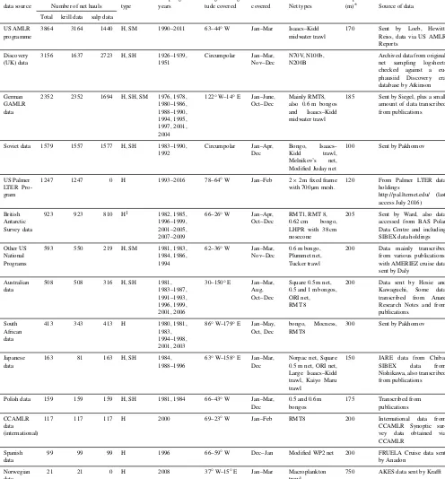
Table 1.Sources of data for KRILLBASE, according to nation and major sampling programme. Sources are listed in descending order of number of hauls provided. More information on the actual data sources (including the references used where data were transcribed from publications) is provided in the SOURCE field of the database. Coverage is not necessarily evenly spread within the longitudinal boundaries, which are presented in nearest integer degrees. For haul type – H: normal haul; SH: stratified haul that has been pooled into an equivalent “stratified pooled haul”. SM: survey mean haul, where density estimates are only available as a mean from multiple stations comprising a survey (see Sect. 2.3).
National Haul Sampling Range of longi- Months Depth
data source Number of net hauls type years tude covered covered Net types (m)∗ Source of data
Total krill data salp data
US AMLR programme
3864 3164 1440 H, SM 1990–2011 63–44◦W Jan–Mar Isaacs–Kidd
midwater trawl
170 Sent by Loeb, Hewitt,
Reiss, data via US AMLR Reports
Discovery (UK) data
3156 1637 2723 H, SH 1926–1939,
1951
Circumpolar Jan–Mar,
Nov–Dec
N70V, N100b, N200B
Archived data from original
net sampling logsheets
checked against a
eu-phausiid Discovery era
database by Atkinson
German GAMLR data
2352 2352 1694 H, SH, SM 1976, 1978,
1980–1986, 1988–1990, 1994, 1995, 1997, 2001, 2004
122◦W–14◦E Jan–June, Oct–Dec
Mainly RMT8, also 0.6 m bongos
and Isaacs–Kidd
midwater trawl
185 Sent by Siegel, plus a small
amount of data transcribed from publications
Soviet data 1579 1557 1577 H, SH 1983–1990,
1992 Circumpolar Jan–Apr, Dec Bongo, Isaacs– Kidd trawl, Melnikov’s net,
Modified Juday net
100 Sent by Pakhomov
US Palmer LTER Pro-gram
1247 1247 0 H 1993–2016 78–64◦W Jan–Feb 2×2 m fixed frame
with 700 µm mesh.
120 From Palmer LTER data
holdings
http://pal.lternet.edu/ (last access July 2016)
British Antarctic Survey data
923 923 810 H1 1982, 1985,
1996–1999, 2001–2005, 2007–2009
66–26◦W Jan–Apr,
Oct–Dec
RMT1, RMT 8,
0.62 cm bongo,
LHPR with 38 cm nosecone
205 Sent by Ward, also data
accessed from BAS Polar Data Centre and including SIBEX data holdings
Other US National Programs
593 550 219 H, SM 1981, 1983,
1984, 1986, 1994
62–36◦W Jan–Mar,
Nov–Dec
0.6 m bongo, Plummet net, Tucker trawl
200 Data mainly transcribed
from various publications, with AMERIEZ cruise data sent by Daly
Australian data
508 508 316 H, SH 1981,
1983–1987, 1991–1993, 1996, 1999, 2001, 2006
30–150◦E Jan–Mar,
Aug, Oct–Dec
Square 0.5 m net, 0.5 and 1 m bongos, ORI net, RMT 8
200 Data sent by Hosie and
Kawaguchi, Some data
transcribed from Anare
Research Notes and from publications.
South African data
413 343 413 H 1980, 1981,
1983, 1994–1998, 2001, 2003
86◦W–179◦E Jan–May,
Oct, Dec
bongo, Mocness,
RMT8
300 Sent by Pakhomov
Japanese data
163 81 163 H, SH 1984,
1988–1996
63◦W–158◦E Jan–Mar, Dec
Norpac net, Square 0.5 m net, ORI net, Large Isaacs–Kidd trawl, Kaiyo Maru trawl
150 JARE data from Chiba,
SIBEX data from
Nishikawa, also transcribed from publications
Polish data 159 159 159 H, SH 1981, 1984 66–43◦W Jan–Mar,
Dec
0.5 and 0.6 m bongos
175 Transcribed from
publications
CCAMLR data (international)
117 117 117 H 2000 69–23◦W Jan–Feb RMT8 200 International data from
CCAMLR Synoptic
sur-vey data obtained via
CCAMLR
Spanish data
99 99 99 H 1996 66–59◦W Dec–Jan Modified WP2 net 200 FRUELA Cruise data sent
by Anadon
Norwegian data
21 21 0 H 2008 37◦W–15◦E Jan–Mar Macroplankton
trawl
750 AKES data sent by Krafft
Other initiatives emphasise the spatial and taxonomic component of data records. For example a previous version of the KRILLBASE data is stored as presence/absence data at SCAR-MarBIN http://www.scarmarbin.be/ (De Broyer et al., 2014). SCAR-MarBIN from the Antarctic node of global-scale initiatives including the Ocean Biogeographical Infor-mation System (OBIS, http://www.iobis.org/) and the Global Biodiversity Information Facility (GBIF, http://www.gbif. org/). Previous versions of KRILLBASE are also available from CCAMLR (https://www.ccamlr.org/) and as part of a gridded global data set of macroplankton biomass (Moriarty et al., 2013). The present version augments this with 50 % more data. If necessary the abundance values can be con-verted to an approximation of biomass (mg C m−3) using, for example, the procedure of Moriarty et al. (2013), who first calculated the number of individuals per m3by dividing den-sity by sampling depth (BOTTOM_SAMPLING_DEPTH_M -TOP_SAMPLING_DEPTH_M), and then applied fixed con-version factors of 63 and 24 mg C ind−1 for krill and salps respectively.
Two of the data sets used in KRILLBASE are available from their respective data websites (http://pal.lternet.edu/ and https://swfsc.noaa.gov/aerd/). Although these do not in-clude the standardised krill abundances available in KRILL-BASE, we refer the user to these two websites to obtain the most up-to-date source data from the Palmer-LTER and US-AMLR time series data. A separate data holding external to KRILLBASE, for example including winter krill data from US SO-GLOBEC, is at BCO-DMO http://www.bco-dmo. org/. The purpose of KRILLBASE is not to duplicate all of these efforts but to bring the krill and salp data together within a single file linked to metadata, in order hopefully to make it more user friendly.
2.3 Structure of KRILLBASE
It is important to differentiate “records” (i.e. rows of the data in KRILLBASE) from “net hauls” and from “sampling sta-tions”. The most common situation is for each record to rep-resent a single net haul at a single station. There is one in-dexing column (labelled “STATION” and 28 further columns (i.e. fields) describing searchable and filterable date, time, position, sampling and environmental information as well as krill and salp abundance. The detailed description of each of these columns is provided in Table 2, while more detail on the nets used for sampling is in Table 3).
While most of the 14 543 records pertain to a single haul made at a station, there are actually four types of record. These are differentiated in the “RECORD_TYPE” column. The most common record, where a single net haul was taken at the station, is simply labelled “haul”. The second cate-gory is labelled “stratified haul”, (2243 records), and these hauls form part of a depth-resolved stratified series made at a station (e.g. 0–50, 50–100, 100–200). The third category is “stratified pooled haul” (567 records) and these pool the
abovementionedstratified haulsinto a single combined “vir-tual haul”, in this example from 0–200 m. The fourth cat-egory (48 records) is labelled “survey mean”. In these the record provides the arithmetic mean abundance from multi-ple stations within a survey. While less than optimal, this ag-gregated information was the only data recoverable from the relevant surveys, which provided data from a valuable 1290 stations during the 1980s.
The krill data are presented as both the observed abun-dance (NUMBER_OF_KRILL_UNDER_1M2, no. m−2) and the abundance standardised relative to a benchmark ( STAN-DARDISED_KRILL_UNDER_1M2, no. m−2), which is ex-plained in Sect. 2.7. The salp data are presented as observed abundance for all species combined, where an individual can be either a solitary oozoid or an individual within an aggre-gate chain (NUMBER_OF_SALPS_UNDER_1M2, no. m−2). Overall there are 15 191 hauls in the database, from 13 542 stations. Of these hauls, 7295 have abundance information on both krill and salps. Others have absent data for either salps or krill, and these are flagged as “not a number” (NaN). This distinguishes it clearly from zero, which indicates that either no krill or no salps were caught. Absent data should therefore not be confused with zeros.
In stratified pooled haul records the NUM-BER_OF_KRILL_UNDER_1M2 and NUM-BER_OF_SALPS_UNDER_1M2 values are the sums of the componentstratified hauls, but are not given (NaN) if data were missing from one or more of thestratified hauls. Location information is generally taken from the deepest component stratified haul. Time information is taken from the shallowest component stratified haul as krill densities are most sensitive to light levels in the surface layers.
2.4 Data processing and error checking
Stations were plotted one survey at a time to identify er-rors in station positions, stations plotting on land, or with latitude and longitudes transposed or with the wrong sign. Implausibly large distances between consecutive sampling points were identified and corrected. Suspiciously low den-sities were identified, based on known or estimated volumes filtered by the various nets and the assumption that no fewer than one krill could have been caught. This procedure iden-tified and led to the correction of a major error made on one portion of the data when converting numbers of krill per 1000 m3to numbers of krill per m−2. Tests of date, time and position coincidence led to the removal of several portions of data that had been entered twice with different station num-bers.
Table 2.Detailed description of the columns in KRILLBASE.
Column heading Description
STATION Unique identifier for each record (row). The first three letters identify the source of the data (starting letters of the name of the individual, national programme, or country which provided the data). The next four numbers identify the season of sampling (e.g. 1926 spans October 1925 to September 1926). The next three letters provide additional sample information, often referring either to the net type used or the name of the sampling survey. Additional characters at the end list the station numbers etc. These are, as far as possible, the same as used in the original sources, with British Antarctic Survey and Palmer LTER cruise station numbers being replaced by cruise-unique “event numbers”. Records are typically resolved to station but see RECORD_TYPE for more information on resolution.
RECORD_ TYPE
This is an important field that will need screening before any use of the database. Records labelled “haul” are the usual situation meaning that the record refers to a single net haul. “Survey mean” represents a record where the krill or salp density represents an arithmetic mean of a group of stations whose central position and sampling point are thus provided in the database with less accuracy then the other records.Survey meansare given only when it was not possible to obtain station-specific data. “Stratified haul” represents a haul, usually within the top 200 m, which forms part of a stratified series (e.g. 0–50, 50–100, 100–200 m). “Stratified pooled haul” represents a record that integrates these respectivestratified hauls, whereby the krill or salp densities from the component nets have been summed (in this example into an equivalent 0–200 m haul). Thus to avoid double counting, any use of the data should sift out eitherstratified haulsorstratified pooled hauls.
NUMBER_ OF_STATIONS
ForSurvey meandata (see RECORD_TYPE) this refers to the number of stations that have been averaged to provide
the krill or salp density values.
NUMBER_ OF_NETS
This refers to the number of sequentially fished nets included in the estimate (e.g. the value would be 3 for a
stratified pooled haulconsisting of a stratified series sampling 0–50, 50–100 and 100–200 m, and it would be 32 for
asurvey meanwhich averages 32 hauls). A LHPR haul counts as one net despite multiple gauzes being cut. This
value is also 1 for a paired bongo haul (two nets fished concurrently).
LATITUDE South is negative. Units are decimal degrees.
LONGITUDE West is negative. Units are decimal degrees.
SEASON This is the austral “summer” season of sampling. For example the 1926 season spans all data from 1 October 1925 through to 30 September 1926.
DAYS_FROM_ 1ST_OCT
This is the day of sampling during the austral season. Therefore 1 October is DAYS_FROM_1ST_OCT=1. The value for dates after 28 February vary depending on whether they occur during a leap year.
DATE The date of sampling, based on the dates provided to us (see “DATE ACCURACY” column).
DATE_ ACCURACY
“D” means the exact day of sampling is known. “M” means that we have been provided only with the month in which samples were taken, so the record’s DATE value is entered as the middle of the month. “Y” means only the year of sampling was provided, so the date is recorded here simply as 1 January (this affects one record only).
NET_TIME This is the time of the haul: either the start, midpoint or end times of hauls were used, as provided to us. Absent data means no net time information was available, or it was not entered into the database because the station was already classified as either day or night (Discovery data net times are recorded in their published “Station Lists” but not entered in KRILLBASE). Net times forStratified pooled haulsrepresent that of the shallowest net of the series.
GMT_OR_ LOCAL
Information on whether the time in the previous column is GMT (labelled “GMT”). Data which were provided as local times with a stated offset to GMT have been converted to GMT. Data which were provided as local times with no offset have not been converted and are labelled “local”. Absent data means there was no net time information.
DAY_NIGHT This field indicates whether the net was hauled in daylight (labelled “day”) or night time (labelled “night”) and was used in the calculation of standardised krill densities. See DAY_NIGHT_METHOD for information on the source of these data.
DAY_NIGHT_ METHOD
Table 2.Continued.
Column heading Description
NET_TYPE This is a brief name for the sampling net used. See Table 3 for more detailed descriptions of each net.
MOUTH_AREA_ OF_NET_M2
This is a nominal mouth area of the net calculated from the net dimensions. It is typically the simple linear area of the mouth, but for RMT8 and 1 it is assigned as value of 8 and 1 respectively. Bongo nets are assigned as an area of both openings combined and LHPR is given as maximum net diameter – both of these are used to crudely compensate for the lack of towing bridles and wire/release gear directly in front of the net, as compared to the standard ring nets often of similar net dimensions.
TOP_SAMPLING_ DEPTH_M
Shallowest sampling depth (m).
BOTTOM_ SAMPLING_ DEPTH_M
Deepest sampling depth (m). Note that whilst most hauls were oblique, double oblique or vertical, a small minority were nearly horizontal, as shown by similar top and bottom depths. These would need to be screened out of nearly all analyses as they provide little information on numerical densities (no. m−2).
VOLUME_ FIL-TERED_M3
Volume of water (m3) filtered by the net. This value is provided only when the value is provided with the density data.
N_OR_S_ POLAR_FRONT
Position (North or South) relative to the Antarctic Polar Front as published by Orsi et al. (1995).
WATER_DEPTH_ MEAN_
WITHIN_10KM
Mean water depth within a 10 km radius. In South Polar Stereographic projection, the stations were superimposed on the Gebco 2014 Grid bathymetry (http://www.gebco.net) and all pixels within a 10 km radius of the station were extracted. After removing data above sea level, the remaining pixel value for water depth was averaged.
WATER_DEPTH_ RANGE_ WITHIN_10KM
Depth range within a 10 km radius. In the procedure above, having removed pixels above sea level, the range in water depth was calculated as the difference between the shallowest and the deepest pixel. This will provide an index of even-ness of bathymetry (e.g. proximity to seamounts, canyons, continental slope).
CLIMATOLO-GICAL_ TEMPERATURE
Long-term average February sea-surface temperature for the sampling location. This is not the actual sea tempera-ture at the time of sampling but a climatological mean sea-surface value for February, averaged over the years 1979 to 2014, based on data downloaded July 2016 from http://apps.ecmwf.int/datasets/data/interim-full-moda/levtype= sfc/. Data were provided on a 0.75◦by 0.75◦grid and we extracted mean values using the same 10 km buffer method used for the bathymetry. These values may indicate a relative thermal regime as a basis for station characterisation.
SD_OF_SURVEY_ MEAN_KRILL
The standard deviation of the krill densities extracted from the publications where thesurvey meanvalue of krill density is provided (see column RECORD_TYPE).
NUMBER_OF_ KRILL_UNDER_ 1M2
Numerical density,N, of numbers of postlarval krill under 1 m2(or, where based on a length frequency distribution as in the Discovery Investigations, it is krill>19 mm in length). Where the numbers of krillnwere provided per m3 filtered, the density of krill was calculated based on top-sampling depthtand bottom-sampling depthbin metres asN=n×(b−t).
STANDARDISED_ KRILL_UNDER_ 1M2
Standardised numerical density of postlarval krill. To reduce possible artefacts arising from differences in sampling method in KRILLBASE, this column presents krill density according to a single sampling method. This method is a 0–200 m night-time RMT8 haul on 1 January, following the standardisation method in Atkinson et al. (2008). See main text for more details.
CAVEATS Any issues which might require particular caution when using the data (e.g. potential inaccuracies in estimated date or day/night or sampling depths outside of the normal range) are listed here. Default is blank.
NUMBER_OF_ SALPS_UNDER_ 1M2
The numerical density of salps, calculated as for krill. All individuals are counted, irrespective of which salp species or whether they are solitaries or components of aggregate chains. Standardised salp densities have not been calcu-lated.
Table 3.Nets used in KRILLBASE. The nets are listed in alphabetical order.
Name given in Nominal mouth Number of Description of net
KRILLBASE area hauls
0.5 m bongo 0.39 23 0.5 m diameter bongo from ABDEX cruises (nominal mouth area is that of both nets)
0.6 m bongo 0.57 1040 0.6 m diameter bongo net (nominal mouth area is of both nets)
0.62 m bongo 0.6 452 BAS bongo: 62 cm diameter (nominal mouth area is of both nets), 0.1 and 0.2 mm mesh
0.71 m bongo 0.79 261 0.71 cm bongo net (Nominal mouth area is of both nets) 1 m ringnet 0.79 111 Modern 1 m diameter ring net
2 m fixed frame net 4 1247 2 m square sided, fixed frame net, 700 µm main mesh, 500 µm cod end (Palmer LTER grid)
IKS net 1 48 IKS 1 mm mesh net, 1 m2, 1 mm mesh
Isaacs–Kidd 3.08 4217 Isaac Kidd midwater trawl, 4.5 mm mesh Juday net 0.11 15 0.37 m diameter Juday net, 0.15 mm mesh
Kaiyu Maru trawl 8 50 Kaiyo Maru midwater trawl (KYMT: 9 and 7 m2 mouth area), 3.4 mm mesh (Nishikawa et al., 1995)
Large Isaacs–Kidd 6 300 Large Isaacs–Kidd trawl including 100 one used for Japanese SIBEX and the 6 m2(4.5 mm mesh) one for Russian/Ukrainian sampling
Large Melnikov net 0.5 17 0.5 m2Melnikov trawl, 0.63 mm mesh
LHPR 0.45 28 Longhurst Hardy Plankton Recorder with 38 cm diameter nosecone used by BAS (0.2 mm mesh)
MOCNESS 1 6 MOCNESS net
Modified Juday net 0.5 694 Modified Juday net, 0.5 m2mouth area, 0.178 mm mesh N100B 0.79 1835 Discovery’s N100B net (1 m diam. ring net)
N200B 3.14 18 N200B net used briefly in 1926 (2 m diameter ring net: soon abandoned as hard to handle)
N70V net 0.39 1396 Discovery’s closing N70V net, also Polish N70V net
Norpac net 0.16 44 0.45 m diameter NORPAC net of JARE expeditions (330 µm net with flowme-ter)
ORI net 2.01 35 Japanese ORI net, 1.6 m diameter mouth, 2 mm mesh Plummet net 1 26 1 m2plummet net used on AMERIEZ (US) cruises in 1980s
RMT1 1 94 RMT 1 net, 0.33 mm mesh
RMT8 8 2753 RMT 8 net, 5 mm mesh
Macroplankton trawl
38 21 “Macroplankton trawl” of research vessel G.O. Sars (AKES data), 3 mm mesh size measured from knot to knot/7 mm stretched mesh. The trawl has the same mesh in all panels from mouth to cod end. Towing speed was 2.5–3 kn. Data and trawl gear is described in Krafft et al. (2010).
Small Melnikov net 0.22 178 0.22 m2Melnikov trawl, 0.63 mm mesh
ORI-VMPS 0.25 85 Square net, 0.5 m across from Australian ANARE and Japanese (Nishikawa and Tsuda, 2001) sampling
Tucker trawl 9 98 Tucker trawl, 4 mm main mesh to a 1 mm cod end, towed at 2 kn. Described in Lancraft et al. (1989)
WP2 0.26 99 WP2 net from Spanish FRUELA cruises
well within expected values (Hamner and Hamner, 2000). The highly patchy spatial distribution of each taxon results in right-skewed frequency distributions, with modes at zero, i.e. no krill caught (Fig. 2). This distribution type is an im-portant consideration in analyses.
Water depths for every net sample were obtained by su-perimposing the stations on a GEBCO_2014 grid, version 20150318, www.gebco.net bathymetry using Arc GIS 10.4.1 and extracting the minimum, mean and maximum water depth within 10 km of each station. The bathymetric
± 500 1000 1500 2000 2500 3000 3500 4000 4500
0 0.4 0.8 1.2 1.6 2 2.4 2.8 3.2 3.6 4 4.4
F
requ
ency
Log10 (NUMBER_OF_KRILL_UNDER_1M2 +1)
Krill abundance
± 500 1000 1500 1000 2500 3000 3500 4000
0 0.4 0.8 1.2 1.6 2 2.4 2.8 3.2 3.6 4 4.4
F
requ
ency
Log10 (STANDARDISED_KRILL_UNDER_1M2 +1)
Standardised krill abundance
± 500 1000 1500 2000 2500 3000 3500
0 0.4 0.8 1.2 1.6 2 2.4 2.8 3.2 3.6 4 4.4
F
requ
ency
Log10 (STANDARDISED_KRILL_UNDER_1M2 +1)
Salp abundance (a)
(b)
[image:9.612.310.545.60.335.2](c)
Figure 2. Frequency distribution of krill and salp abundances in the database. The data were filtered to removestratified hauls be-fore plotting the frequency of remaining hauls in relation to loga-rithmic bins. Data are presented for(a)krill raw (unstandardised) abundance,(b)krill standardised abundance and(c)salp (unstan-dardised) abundance.
catches were from warmer waters north of the Antarctic Po-lar Front, giving grounds for suspicion, for example of iden-tification. We kept these records since expatriated individuals are a possibility and we did not want to judge the data pro-vided. Data caveat issues are indicated and described in the fields DATE_ACCURACY and CAVEATS respectively.
2.5 Variation in sampling coverage and method
[image:9.612.69.268.63.358.2]Figure 1 shows that KRILLBASE sampling is highly uneven, focusing on areas of fishing or historical interest to nations in the Atlantic sector (USA, Germany, UK, Poland, South Africa, Spain) or Indian sectors (Soviet Union, Japan, Aus-tralia). While Fig. 1 plots the stations with either krill or salp data or both, Fig. S1 in the Supplement plots only those sta-tions with krill data. Data compilation was mainly focused on the Antarctic zone; 765 records are north of the Antarctic Po-lar Front. “Discovery” sampling (i.e. those data obtained as part of the Discovery Investigations in the 1920s and 1930s) started nearer South Georgia and became increasingly cir-cumpolar but, despite this, major gaps in sample coverage
Figure 3.Circumpolar variation in sampling method. This plot is based on all data in KRILLBASE, whether for krill or salps or both. (a)Time of year of sampling (mean day from 1 October).(b) Bot-tom depth of sampling. The data set plotted includes the stratified pooled hauls and thus excludes their component stratified hauls (see Sect. 2.3).(c)Mean mouth area of the net, based on the nominal values presented for each net type in Table 3. Antarctic Polar Front position is from Orsi et al. (1995).
exist in important areas such as the Ross Sea, Weddell Sea and in large parts of the Pacific sector.
The composite nature of KRILLBASE means that the sampling methods vary. Figure 3 illustrates this with a cir-cumpolar comparison of the seasonal timing of sampling (Fig. 3a), bottom depth of sampling (Fig. 3b) and mouth area of the net (Fig. 3c). Time of year of sampling has a poten-tially strong influence on the abundance of zooplankton, due to life cycle and behavioural traits such as seasonal vertical migration (Foxton, 1966; Atkinson et al., 2012a; Cleary et al., 2016). While samples were obtained during most months of the year, 89 % of the hauls were conducted in the period December to March (Fig. 4), with no longitudinal bias in tim-ing (Fig. 3a). However, in sparsely sampled areas, particu-larly north of the Antarctic Polar Front, sample timing varied greatly, underlining the caution needed in interpreting these samples. The original objectives for using KRILLBASE did not require winter samples but some winter data are available from several key surveys (e.g. http://www.bco-dmo.org/) and could be included in subsequent updates of KRILLBASE.
Figure 4.Relative frequency of stations sampled within each month of the year.
Figure 5. Vertical distribution of krill and salps based on 793 stratified krill hauls and 2130 stratified salp hauls. Given the non-standard depth horizons between the various surveys sampling in this manner, the data were first subdivided into a nominal seven categories of mean sampling depths, namely 0–50, 50–100, 100– 150, 150–200, 200–300, 300–500 and>500 m. Mean krill or salp densities are presented in each of these mean depth groups, plotted against mean sampling depth within each depth band.
greatly between the component surveys, as indicated by the chequered colours of Fig. 3b. Some screening by the user is necessary to remove stations where an unrepresentative portion of the depth distribution was covered. Figure 5 sum-marises the vertical distribution of krill and salps where strat-ified series of net hauls were undertaken (269 krill stations and 563 salp stations). This shows the highest densities of krill in the top 200 m, with declining densities below this. KRILLBASE is suitable for exploring the horizontal distri-bution of krill in the important epipelagic zone, but is un-suitable to map horizontal distribution below 200 m. These deeper and near- seabed zones are being increasingly recog-nised as important habitats for krill (Gutt and Siegel, 1994; Clarke and Tyler, 2008; Schmidt et al., 2011; Cleary et al., 2016).
Salps have a deeper distribution than krill (Fig. 3) as a re-sult of greater diel and seasonal vertical migrations (Foxton, 1966; Loeb and Santora, 2012). Care is therefore needed to avoid negative bias due to shallow net sampling. A
standardi-Figure 6.Inter-annual sampling coverage. Number of stations sam-pled south of the Antarctic Polar Front in each austral season (Oc-tober to following September). These are presented for(a)the At-lantic sector (nominally defined as 90◦W–10◦E), (b) the Indian sector (10–120◦E) and(c)the Pacific sector (120◦E–90◦W).
sation method similar to that applied to krill may reduce these inconsistencies and provide a better picture of the spatial dis-tribution of salps.
2.6 Inter-annual coverage
Figure 6 divides the Southern Ocean into broad sectors to il-lustrate the inter-annual coverage of sampling. The coverage for salps broadly follows that for krill, with good coverage in the Atlantic sector from 1926 to 1938 and after 1976. In the Indian Ocean sector some data exist from the late 1930s when “Discovery” sampling became circumpolar, reasonable coverage occurred from 1981 to the mid-1990s, but few data have been collected there since. While coverage in the Pacific sector is too sporadic to document time trends, data for the other two sectors are sufficient to examine sectorial patterns of inter-annual and decadal-scale variability of both krill and salps.
[image:10.612.68.267.236.372.2]0 0.1 0.2 0.3 0.4 0.5 0.6 0.7 0.8 0.9 1
0 50 100 150 200 250
D a y l e n g th ( a s a p ro p o rt io n o f 2 4 h )
[image:11.612.82.251.66.218.2]Days after 1 October Lat 50° S Lat 55° S Lat 60° S Lat 65° S
Figure 7.Change in day length with time of year at various lati-tudes, indicating the effect of date inaccuracies on time of day ad-justments made during standardisation of krill abundance.
monitoring programmes. These data can be included in re-gional scale analyses (e.g. time series analyses), but since the data pertain only to the whole survey and not the component stations, care is needed when interpreting the data at finer scales than the 3◦latitude by 9◦longitude grids illustrated.
2.7 Standardisation: methods
The compiled data represent a range of sampling methods with different net types, sampling depths, times of day and times of year (Fig. 3). Such differences in sampling strategy could potentially bias the outcome of analyses. For exam-ple, differences in net mouth size will lead to variable avoid-ance and the mesh size will affect retention. Differences in net geometry, towing speed and trajectory will further af-fect catches, as will light levels and swarm packing density (Hamner and Hamner, 2000; Everson and Bone, 1986; Krag et al., 2014). For example, catchability decreases as light levels increase, meaning that there can be a latitudinal ef-fect because summer days are much longer at high latitudes (Fig. 7). These issues were recognised by Marr (1962) and Mackintosh (1973), who adjusted the densities accordingly when producing circumpolar distribution maps.
To minimise the influence of sampling differences, our database includes both the raw numerical abundances of krill and values standardised to a single sampling method. We cal-culated the standardised krill abundances using the process and conversion factors described in the supplementary ap-pendix of Atkinson et al. (2008). The standardised abundance (STANDARDISED_KRILL_UNDER_1M2) is an estimate of the krill abundance that would have been observed if the haul had conformed with a sampling method consisting of a night-time haul on 1 January, fishing to a depth of 200 m with a mouth area of 8 m2. This strategy achieves near-maximum krill catch that is possible with scientific nets.
T ab le 4. Summary of standardisation process. Standardise for Standard haul characteristics Con v ersion factor Definitions Con v ersion factor applied when: Sampling depth 0–200 m 0.11B / (1 + 0.105B) B = BO TT OM_SAMPLING_ DEPTH_M BO TT OM_SAMPLING_ DEPTH_M < 200 T ime of day Night-time 2.255 D A Y_NIGHT = 0 (day time) 2.255 X X = NEW_D A YLENGTH (specified as a proportion) D A Y_NIGHT = blank (no information) Net mouth area and time of year of sampling Net mouth area = 8 m 2 T ime of year = 1 January L opt pred /K pred Kpred = P × Knon − zero P = exp( L ) / [ 1 + exp( L ) ] Log 10 ( Knon − zero ) = 0 . 474 − 0 . 1912Log 10 M + 0 . 00416 J − 0 . 00002898 J 2 L = − 0 . 6478 + 2 . 335 × Log 10 M + 0 . 0204 J − 0 . 0001086 J 2 M = MOUTH_AREA_OF_NET_M3 J = JULIAN_D A Y_FR OM_OCT L opt pred = Popt × K opt non − zero Popt = 0 . 92 K opt non − zero = 2.74 MOUTH_AREA_OF_NET_M3 <> 8
or DA
YS_FR
OM_1st_OCT
<>
Table 5.Derivation ofDay or nightinformation.
Information available Information used to stan-dardise time of day
ValidNet time(GMT, or Local with specified offset)
Calculate solar elevation and use to determineDay or night
No valid Net time but valid day or night information from ship’s log (values 0 or 1)
Use ship’s log informa-tion to indicate Day or night
No validNet timeor ship’s log information (e.g. when a Local time is specified but no offset is given, and the ship’s log does not specify day or night or in-dicates twilight)
CalculateDay-lengthand use to adjust conversion factor
Standardisation was implemented by multiplying the raw abundances (NUMBER_OF_KRILL_UNDER_1M2, N) by conditional conversion factors as follows:
N0=N 0.11B
1+105B2.255X
2.5208
Kpred,
whereN0is the standardised krill abundance,Bis the bottom sampling depth,Xis a scalar to adjust the day-to-night con-version factor (2.255) andKpred is the expected krill abun-dance based on a general linear model in which mouth area and time of year are the independent variables (see Table 4 and Atkinson et al., 2008, for further details). X=1 when the net was hauled in daylight andX=1/2.255 when it was hauled at night. We also calculated standardised krill densi-ties for nets where there was insufficient information to de-termine whether hauling occurred in daylight or at night. In these cases the value ofXis the probability that the net was hauled in daylight (i.e. day length in hours/24).
The revision of KRILLBASE included reassessment of the DAY_NIGHT field (indicating whether the net was hauled in the daylight or at night; see Table 5). Where valid sam-pling time information was available (consisting of a GMT NET_TIME or a local NET_TIME and sufficient informa-tion to adjust to GMT), we used the Twilight Excel work-book available from http://www.ecy.wa.gov/programs/eap/ models.html to determine whether the haul was conducted in daylight (defined by a solar elevation>−0.833◦). Where no valid sampling time information was available, but there was an indication of day or night in the original data, we used this information. Where it was not possible to make this assessment because of insufficient information, we used the TwilightExcel workbook to calculate day length for the sam-pling date and location, which was then used to adjust the standardised krill density as described above. As this type of standardised krill abundance (indicated by a value of 3 in the DAY_NIGHT_METHOD field) uses a different time of
day adjustment from other standardised krill abundances it is good practice to assess its influence on results.
2.8 Standardisation: caveats on the use of standardised krill densities
KRILLBASE includes standardised krill abundance informa-tion for every haul, stratified pooled haul and survey mean except those with TOP_SAMPLING_DEPTH_M deeper than 50 m (because hauls which exclude the surface layers are not comparable with those that include these layers). These standardised densities will be most reliable when the information underlying the standardisation is accurate. Thus where dates or times have been estimated (for example for survey meandata) the database provides information on the accuracy of date information (DATE_ACCURACY) and the type of time information (DAY_NIGHT_METHOD) avail-able in each record.
Although the ideal method for depth standardisation is to make all hauls equivalent to a haul sampling from 0 to 200 m depth, the standardisation described in Atkinson et al. (2008) and used here, is a partial solution which standard-ises bottom-sampling depth to 200 m when the actual value is less than 200 m. It does not exclude krill caught deeper than 200 m, where krill densities are generally lower (Schmidt et al., 2011), nor does it adjust for nets that did not sam-ple to the surface (TOP_SAMPLING_DEPTH greater than 0 m). Users are advised to screen the data to ensure that top-sampling depths are consistent with their requirements, not-ing that there are 691haulsin the current version of KRILL-BASE have top-sampling depths deeper than 5 m and Atkin-son et al. (2008) excluded such hauls before calculating the conversion factors.
Date information affects the standardisation through the adjustments for time of year and time of day. Atkinson et al. (2008) derived the conversion factors from a data set where the latest sampling date was 26 April. Recent KRILL-BASE updates include hauls taken as late as 30 August, but we have not provided standardised krill densities for sam-pling dates after 30 April because the standardisation is ex-tremely sensitive to dates after this point (e.g. the time-of-year adjustment for 30 August increases krill density by a factor of 3834, compared to a factor of 10 for 26 April, and a factor of 1.16 for 31 January). This strong effect of time of year of sampling on abundance likely reflects both mortal-ity and seasonal vertical migration of krill out of the surface layer late in the season (Cleary et al., 2016)
con-Figure 8.Circumpolar distribution maps of krill based on(a) un-standardised krill densities (no. m−2),(b)standardised krill densi-ties and(c)unstandardised salp densities, showing the stations sam-pled for these. All maps are South Polar Stereographic projection with grid size of 3◦latitude by 9◦longitude. Positions of krill sta-tions are in Fig. S1 in the Supplement. The legend values and colour codings of cells refer to the arithmetic mean krill densities recorded within the cell.
sequence and true dates closer to 1 January will be treated less conservatively. The effect of any date inaccuracies in-creases with time from 1 January. TheDATA_CAVEATSfield in the database clearly indicates for each row which, if any, of the above caveats applies.
3 Results and discussion
3.1 Effects of heterogeneous data sources and standardisation: spatial effects
Figure 8 compares the circumpolar distribution of krill and salps, allowing a comparison between the standardised and unstandardised krill values obtained from KRILLBASE. While hauls with zero krill remained as such, median stan-dardised krill abundance of positive hauls was 2.2 times greater than that of unstandardised values. The overall cir-cumpolar pattern of relative abundance is similar whether based on raw or standardised abundances but the detail in some areas does differ. This is likely due to longer sum-mer days at higher latitudes (requiring upwards adjustment of most catches to night values) or the localised use of poor sampling combinations (e.g. smaller nets and/or early or late season sampling).
The patchy distributions of krill and salps and spatial dif-ferences in sampling density influence the spatial patterns shown in the maps. A few grid cells suggest extremely high krill or salp abundance, but some of these cells only include a few stations. Conversely, cells suggesting absence frequently have too few stations for a reliable picture. Users need to allow for variable sampling coverage, and while our stan-dardisation attempts to reduce net sampling inconsistencies, it does not adjust for variable precision.
3.2 Effects of heterogeneous data sources and standardisation: temporal effects
The South Georgia area exemplifies the krill-based ecosys-tem and this has been sampled for many years (Murphy et al., 2007). We have therefore selected a subset of KRILLBASE in this area to show how sampling method can vary from year to year and how this could affect time trends (Fig. 9). This area has been sampled with a wide variety of methods since the 1920s, and the mean krill abundance varies greatly from year to year due to recruitment variability (Fig. 9a; see also Murphy et al., 2007; Fielding et al., 2014). While the stan-dardised annual mean krill abundances are typically greater than the unstandardised values, the offset varies substantially. This is for a number of reasons, including variable mouth areas and sampling depths of the net (Fig. 9b) and variable time of year and time of day of sampling (Fig. 9c). For exam-ple, net mouth area is generally larger (albeit more variable) in the modern post-1970s era, concomitant with an increase in bottom-sampling depth of the nets. Likewise, during the modern era, the proportions of hauls in mid-summer and at night have increased.
The above factors are included in the standardisation pro-cess, but other issues may be important when deciding how to screen data and interpret time trends from a heterogeneous data set such as KRILLBASE. One factor is the density of sampling coverage within any given year. We have not plot-ted years when there are very few stations sampled (<10 sta-tions) because a patchy swarming species like krill is likely to be missed altogether by such limited sampling. However, the number of stations sampled varies greatly from year to year (Fig. 6) so we have scaled the size of the symbols according to numbers of stations to illustrate the variable confidence in the annual means.
[image:13.612.49.286.63.303.2]Figure 9.Inter-annual variability in sampling. Year-to-year varia-tion in net sampling, and its effect on the difference between stan-dardised and unstanstan-dardised krill density. Austral season is plot-ted on thexaxis of all panels with a vertical line demarcating the Discovery sampling era from the post-1975 sampling era.(a) inter-annual variation in arithmetic mean krill densities in the greater South Georgia area (30–40◦W, 50–60◦S, based on hauls from October to April with a top-sampling depth<20 m and bottom-sampling depth>50 m following Atkinson et al., 2008). While we have not plotted data with fewer than 10 hauls in any year, the sym-bols are in three sizes to illustrate the variability in sampling effort – smallest: 10–20; medium: 20–50; and largest>50 hauls per sea-son.(b)Inter-annual variability in mean mouth area of the net and mean bottom-sampling depth of the net from the hauls in panel(a). (c) Inter-annual variability in Julian day of sampling (days from 1 October) and the percentage of night-time hauls.(d)Percentage of hauls over continental shelves of the sampling area, defined as water depth<1000 m.
Figure 10.Basin-scale krill(a, b)and salp distribution(c, d)within two well-studied sectors of the Southern Ocean, plotted on a finer, 1◦latitude by 2◦longitude grid to highlight habitat differences be-tween the two taxa.
while monitoring in the 1990s and 2000s was more shelf-orientated.
4 Data availability
[image:14.612.92.236.67.479.2]sources (Table 1) regarding queries. This data paper in ad-dition to the data doi should be cited as the metadata and the source of the data, to allow traceability in the use of this database. This will hopefully provide leverage for obtaining future funding to continue rescuing and updating valuable historical data sets from the Southern Ocean. As a final word we urge users to take a few minutes to consult the metadata, in particular Table 2, since almost every use of KRILLBASE will require an initial screening of some of the records.
5 Conclusions and recommendations
5.1 Uses and limitations of KRILLBASE
The first version of KRILLBASE was used by Atkinson et al. (2004) to quantify the circumpolar distribution of krill and salps, examine regional trends in their densities and de-termine inter-annual relationships between krill density and winter sea ice cover. Inter-annual changes in mean krill abun-dance were subsequently related to temperature by White-house et al. (2008), to whale dynamics by Braithwaite et al. (2015) and to the dynamics of other so-called wasp-waist species by Atkinson et al. (2014). The fact that krill and salp abundances vary so much between years is an advan-tage for this inter-annual scale of analysis, because the signal is stronger than the noise.
The spatial component of KRILLBASE has been used more widely. Circumpolar distributions have been used as a context and validation for various models and analyses including biogeochemical carbon cycling (Moriarty, 2009), krill and climate change (Flores et al., 2012; Hill et al., 2013; Piˇnones and Federov, 2016), population connectivity (Thorpe et al., 2007; Siegel and Watkins, 2016), predator for-aging (Pangerc, 2010) and vertical and horizontal krill habitat analyses (Atkinson et al., 2008; Schmidt et al., 2011). These studies have tended to focus on large scales, but smaller-scale analyses of well-sampled areas (as shown in Fig. 10) are amenable to KRILLBASE, for example to interpret preda-tor foraging areas. The caveat here is that these maps are not synoptic, but instead are more akin to probability maps of where krill or salps occur, providing a context for more syn-optic snapshots from surveys (Siegel et al., 2004; Kawaguchi et al., 2004).
In parallel to expansion of the abundance component of KRILLBASE, we are generating a large database on krill length frequency, sex, and maturity stage from scientific and fisheries data, a work still in progress. Combining the length frequency and abundance components provides insights into biomass and production at large scales, allowing a degree of scaling-up of acoustics-derived biomass surveys (Atkinson et al., 2009). The sex/length frequency component has since been used, for example, to relate circumpolar trends in body length to feeding conditions (Schmidt et al., 2014), and to ex-amine sex-related changes in seasonal growth and shrinkage (Tarling et al., 2016).
In comparison to krill, fewer studies have used the salp component of KRILLBASE. Lee et al. (2010) examined inter-annual variability in krill and salps simultaneously, em-phasising the opposite nature of the trends observed in the two taxa. Given the fact that about half of the current KRILL-BASE net hauls have both krill and salps recorded, a simul-taneous evaluation of the two taxa would be valuable. In any of these analyses, however, we emphasise that great care is needed when interpreting time trends, in order to prevent aliasing of real patterns with differences in sampling meth-ods. This applies equally to salps and to krill, for example, the seasonal and diel vertical migrations of salps mean they are prone to under-sampling by shallow nets (Fig. 4).
An additional caveat concerns the issues of net sampling efficiency for mobile species such as krill. RMT8 catches during night-time were set as our benchmark for standard-isation because they were the most efficient means of cap-turing krill, but even these catches were likely to have un-derestimated absolute abundance. This is due to both net avoidance and escapement of the smallest juveniles through the meshes. Nevertheless, the overall circumpolar biomass of krill based on averaged KRILLBASE data is 379 Mt, so it is unlikely that this sampling method is yielding order of mag-nitude underestimates (Atkinson et al., 2009). KRILLBASE may provide insights on the relative distribution and tempo-ral variation in krill density, but modern acoustic methods calibrated with nets are the accepted method for determining krill biomass (Fielding et al., 2014). Integrating the assess-ments from these two fundamentally different types of sam-pling represents the most robust practice to achieve large-scale and long-term estimates of krill biomass.
The Supplement related to this article is available online at doi:10.5194/essd-9-193-2017-supplement.
Author contributions. A. Atkinson, S. L. Hill, E. A. Pakhomov and V. Siegel are the instigators of KRILLBASE or this project to produce the data paper, and are listed in alphabetical order. The re-maining authors are contributors to the database and the current paper, also listed in alphabetical order. Original concept and ini-tial database: A. Atkinson, V. Siegel, and E. A. Pakhomov. Addi-tional data sets: V. Loeb, C. S. Reiss, D. K. Steinberg, L. B. Quetin, R. M. Ross, P. Ward, S. Kawaguchi, G. W. Hosie, S. Fielding, S. Chiba, J. Nishikawa, R. Anadon, and B. A. Krafft; Data check-ing, manipulation, spatial analysis, standardisation and editing: A. Atkinson, S. L. Hill, R. C. Subramaniam, H. J. Peat, L. Gerrish, P. Fretwell, M. J. Jessopp, K. Schmidt, V. Siegel, and E. A. Pakho-mov. Final maps: L. Gerrish. Final data-basing: H. J. Peat; Drafting manuscript: S. L. Hill, and A. Atkinson. Input to manuscript: all.
Acknowledgements. We are greatly indebted to the crews and scientists who have collected thousands of net samples over the last 90 years, analysed the catches, and then provided data in a format that is useable. Boris Trotsenko was a major facilitator in rescuing old Soviet Union data. Marie-Fanny Racault accessed satellite tem-perature climatology data and Janet Silk helped with spatial data checks. We are grateful to Peter Rothery for the original standardis-ation of the krill density data. D. K. Steinberg acknowledges the US National Science Foundation (grant PLR-1440435). B. A. Krafft was supported by the Royal Norwegian Ministry of Fisheries and Coastal affairs, the Institute of Marine Research, the University of Bergen, the Norwegian Antarctic Research Expeditions (NARE), the Norwegian Research Council, Statoil Hydro and the Norwegian Petroleum Directorate. In the last 5 years the funding to update the database was via the Antarctic Climate and Ecosystem Cooperative Research Centre (for R. C. Subramaniam) and the UK Natural Environment Research Council and Department for Environment, Food and Rural Affairs grant NE/L003279/1, Marine Ecosystems Research Program (for Angus Atkinson). After this the final production of the database and creation of this data paper was funded by the World Wildlife Fund.
Edited by: F. Huettmann
Reviewed by: T. O’Brien and two anonymous referees
References
Atkinson, A., Siegel, V., Pakhomov, E., and Rothery, P.: Long-term decline in krill stock and increase in salps within the Southern Ocean, Nature, 432, 100–103, 2004.
Atkinson, A., Siegel, V., Pakhomov, E. A., Rothery, P., Loeb, V., Ross, R. M., Quetin, L. B., Fretwell, P., Schmidt, K., Tarling, G. A., Murphy, E. J., and Fleming, A.: Oceanic circumpolar habitats of Antarctic krill, Mar. Ecol. Prog. Ser., 362, 1–23, 2008. Atkinson, A., Siegel, V., Pakhomov, E. A., Jessopp, M. J., and Loeb,
V: A re-appraisal of the total biomass and production of Antarctic krill, Deep-Sea Res. Pt. I, 56, 727–740, 2009.
Atkinson, A., Ward, P., Hunt, B. P. V., Pakhomov, E. A., and Hosie, G. W.: An overview of Southern Ocean zooplankton data: abun-dance, biomass, feeding and functional relationships, CCAMLR Science, 19, 171–218, 2012a.
Atkinson, A., Nicol, S., Kawaguchi, S., Pakhomov, E. A., Quetin, L. B., Ross, R. M., Hill, S. L., Reiss, C., Siegel, V., and Tarling, G.: Fitting Euphausia superbainto Southern Ocean food-web models: a review of data sources and their limitations, CCAMLR Science, 19, 219–245, 2012b.
Atkinson, A., Hill, S. L., Barange, M., Pakhomov, E. A., Rauben-heimer, D., Schmidt, K., Simpson, S. J., and Reiss, C.: Sardine cycles, krill declines and locust plagues: revisiting “wasp-waist” food webs, Trends Ecol. Evol., 29, 309–316, 2014.
Atkinson, A., Hill, S. L., Pakhomov, E. A., Siegel, V., Anadon, R., Chiba, S., Daly, K. L., Downie, R., Fielding, S., Fretwell, P., Gerrish, L., Hosie, G. W., Jessopp, M. J., Kawaguchi, S., Krafft, B. A, Loeb, V., Nishikawa, J., Peat, H. J., Reiss, C. S., Ross, R. M., Quetin, L. B., Schmidt, K., Steinberg, D. K., Sub-ramaniam, R. C., Tarling, G. A., and Ward, P.: The KRILL-BASE (1926–2016) Antarctic krill and salp abundance database, doi:10.5285/8b00a915-94e3-4a04-a903-dd4956346439, 2016.
Braithwaite, J. E., Meeiwig, J. J., Letessier, T. B., Jenner, K. C. S., and Brierley, A. S.: From sea ice to blubber: linking whale con-dition to krill abundance using historical whaling records, Polar Biol., 38, 1195–1202, 2015.
Clarke, A. and Tyler, P. A.: Adult Antarctic krill feeding at abyssal depths, Curr. Biol., 18, 282–285, 2008.
Constable, A. J.: Lessons from CCAMLR on the implementation of the ecosystem approach to managing fisheries, Fish Fish., 12, 138–151, 2011.
Cleary, A., Durbin, E. G., Cesas, M. C., and Zhou, M. : Winter dis-tribution and size structure of Antarctic krillEuphausia superba populations in-shore along the West Antarctic Peninsula, Mar. Ecol. Prog. Ser., 552, 115–129, doi:10.3354/meps11772, 2016. De Broyer, C., Koubbi, P., Griffiths, H. J., Raymond, B., Udekemd
Acoz, C., Van de Puitte, A. P., Danis, B., David, B., Grant, S., Gutt, J., Held, C., Hosie, G., Huettmann, F., Post, A., and Ropert-Coudert, Y. (Eds.): Biogeographical Atlas of the South-ern Ocean, Scientific Committee for Antarctic Research, Cam-bridge, 498 pp., 2014.
De la Mare, W.: Abrupt mid-twentieth century decline in Antarctic sea-ice extent from whaling records, Nature, 389, 57–60, 1997. Everson, I. and Bone, D. G.: Effectiveness of the RMT 8 system
for sampling krill (Euphausia superba) swarms, Polar Biol., 6, 83–90, 1986.
Fielding, S., Watkins, J. L., Trathan, P. W., Enderlein, P., Waluda, C. M., Stowasser, G., Tarling, G. A., and Murphy, E. J.: Interan-nual variability in Antarctic krill (Euphausia superba) density at South Georgia, Southern Ocean: 1997–2013, ICES J. Mar. Sci., 71, 2578–2588, doi:10.1093/icesjms/fsu104, 2014.
Flores, H., Atkinson, A., Rebolledo, E., Cirelli, V., Cuzin-Roudy, J., Fielding, S., van Franeker, J. A., Groeneveld, J. J., Haralds-son, M., Kawaguchi, S., Krafft, B. A., Lombana, A., Marschoff, E., Meyer, B., Milinevsky, G., Nicol, S., Pakhomov, E. A., Vande Putte, A. P., Reiss, C., Rombolá, E., Schmidt, K., Siegel, V., Tar-ling, G. A., Teschke, M., Tonkes, H., Toullec, J.-Y., Trathan, P. N., Tremblay, N., Werner, R., and Werner, T.: Impact of climate change on Antarctic krill, Mar. Ecol. Prog. Ser., 458, 1–19, 2012. Foxton, P.: The distribution and life history ofSalpa thompsoni Fox-ton, with observations on a related species,Salpa gerlachei Fox-ton, Discovery Reports, 34, 1–116, 1966.
Gutt, J. and Siegel, V.: Benthopelagic aggregations of krill (
Euphau-sia superba) on the deeper shelf of the Weddell Sea, Deep-Sea
Res., 141, 169–178, 1994.
Gille, S. T.: Warming of the Southern Ocean since the 1950s, Sci-ence, 295, 1275–1277, 2002.
Gillett, N. P. and Fyfe, J. C.: Annular mode changes in the CMIP5 simulation, Geophys. Res. Lett., 40, 1189–1193, doi:10.1002/grl.50249, 2013.
Gleiber, M. R., Steinberg, D. K., and Ducklow, H. W.: Time series of vertical flux of zooplankton fecal pellets on the continental shelf of the western Antarctic Peninsula, Mar. Ecol. Prog. Ser., 471, 23–36, 2012.
Grant, S. M., Hill, S. L., Trathan, P. N., and Murphy, E. J.: Ecosys-tem services of the Southern Ocean: trade-offs in decision-making, Antarctic Science, 25, 603–617, 2013.
Hamner, W. M. and Hamner, P. P.: Behavior of Antarctic krill (
Eu-phausia superba): schooling, foraging, and antipredatory
Hill, S. L. and Cannon, M.: A potential feedback approach to ecosystem-based management: model predictive control of the Antarctic krill fishery, CCAMLR Sci., 20, 119–137, 2013. Hill, S. L., Phillips, A., and Atkinson, A.: Potential climate
change effects on the habitat of Antarctic krill in the Wed-dell quadrant of the Southern Ocean, PLoS One, 8, e72246, doi:10.1371/journal.pone.0072246, 2013.
Hill, S., Cavanagh, R., Knowland, C., Grant, S., and Downie, R.: Bridging the krill divide: understanding cross-sector objectives for krill fishing and conservation, British Antarctic Survey, Cam-bridge, 2014.
Jarman, S. N. and Deagle, B. E.: Genetics of Antarctic krill, in: The biology and ecology of Antarctic krill,Euphausia superbaDana, 1850, edited by: Siegel, V., Springer, Dordrecht, the Netherlands, 247–278, 2016.
Kawaguchi, S., Siegel, V., Litvinov, F., Loeb, V., and Watkins, J.: Salp distribution and size composition in the Atlantic sector of the Southern Ocean, Deep-Sea Res. Pt. II, 51, 1369–1381, 2004. Kinzey, D., Watters, G. M., and Reiss, C. S.: Selectivity and two biomass measures in an age-based assessment of Antarctic krill
(Euphausia superba), Fisheries Res., 168, 72–84, 2015.
Krafft, B. A., Melle, W., Knutsen, T., Bagøien, E., Broms, C., Ellert-sen, B., and Siegel, V.: Distribution and demography of Antarctic krill in the Southeast Atlantic sector of the Southern Ocean dur-ing the austral summer 2008, Polar Biol., 33, 957–968, 2010. Krafft, B. A., Skaret, G., Krag, L. A., Rustand, T., and Pedersen,
R.: Antarctic krill and ecosystem monitoring survey at South Orkney Islands in 2016, Institute of Marine Research Report No. 20, 22 pp., 2016.
Krag, L. A., Herrmann, B., Iversen, S. A., Engås, A., Nor-drum, S., and Krafft, B. A.: Size selection of Antarctic krill (Euphausia superba) in trawls, PLoS ONE, 9, e102168, doi:10.1371/journal.pone.0102168, 2014.
Lancraft, T. M., Torres, J. J., and Hopkins, T. L.: Micronekton and macrozooplankton in the open waters near Antarctic ice edge zones (AMERIEZ 1983 and 1986), Polar Biol., 9, 225–233, 1989.
Lee, C. I., Pakhomov, E. A., Atkinson, A., and Siegel, V.: Long-term relationships between the marine environment, krill and salps in the Southern Ocean, J. Mar. Biol., 2010, 410129, doi:10.1155/2010/410129, 2010.
Loeb, V., Siegel, V., Holm-Hansen, O., Hewitt, R., Fraser, W., Triv-elpiece, W., and TrivTriv-elpiece, S.: Effects of sea-ice extent and kril-lor salp dominance on the Antarctic food web, Nature, 387, 897– 900, 1997.
Loeb, V. J. and Santora, J. A.: Population dynamics of Salpa
thompsoni near the Antarctic Peninsula: growth rates and
in-terannual variations in reproductive activity (1993–2009), Progr. Oceanogr., 96, 93–107, 2012.
Loeb, V. J. and Santora, J. A.: Climate variability and spatiotem-poral dynamics of five Southern Ocean krill species, Progr. Oceanogr., 134, 93–122, 2015.
Marr, J. W. S.: The natural history and geography of the Antarc-tic krill (Euphausia superbaDana), Discovery Rep., 32, 33–464, 1962.
Mackintosh, N. A.: Distribution of post-larval krill in the Antarctic, Discovery Rep., 36, 1–94, 1973.
Meredith, M. P. and King, J. C.: Rapid climate change in the ocean west of the Antarctic Peninsula during the second
half of the 20th century, Geophys. Res. Lett., 32, L19604, doi:10.1029/2005GL024042, 2005.
Moriarty, R.: The Role of Macrozooplankton in the Global Car-bon Cycle, PhD Thesis, University of East Anglia, Norwich, UK, 2009.
Moriarty, R., Buitenhuis, E. T., Le Quéré, C., and Gosselin, M.-P.: Distribution of known macrozooplankton abundance and biomass in the global ocean, Earth Syst. Sci. Data, 5, 241–257, doi:10.5194/essd-5-241-2013, 2013.
Murphy, E. J., Watkins, J. L., Trathan, P. N., Reid, K., Meredith, M. P., Thorpe, S. E., Johnston, N. M., Clarke, A., Tarling, G. A., Collins, M. A., Forcada, J., Shreeve, R. S., Atkinson, A., Korb, R., Whitehouse, M. J., Ward, P., Rodhouse, P. G., Enderlein, P., Hirst, A. G., Martin, A. R., Hill, S. L., Staniland, I. J., Pond, D. W., Briggs, D. R., Cunningham, N. J., and Fleming, A. H.: Spatial and temporal operation of the Scotia Sea ecosystem: a review of large-scale links in a krill centered food web, Philos. T. Roy. Soc. B, 362, 113–148, 2007.
Murphy, E. J., Clarke, A., Abram, N. J., and Turner, J.: Variability of sea-ice in the northern Weddell Sea during the 20th century, J. Geophys. Res.-Oceans, 119, 4549–4572, 2014.
Nishikawa, J. and Tsuda, A.: Diel vertical migration of the pelagic tunicate,Salpa thompsoniin the Southern Ocean during the aus-tral summer, Polar Biol., 24, 299–302, 2001.
Nishikawa, J., Naganobu, M., Ichii, T., Ishii, H., Terazaki, M., and Kawaguchi, K.: Distribution of salps near the South Shetland Is-lands during austral summer, 1990–1991 with special reference to krill distribution, Polar Biol., 15, 31–39, 1995.
Orsi, A. H., Whitworth, T., and Nowlin, W. D.: On the meridional extent and fronts of the Antarctic Circumpolar Current, Deep-Sea Res. Pt. I, 42, 641–673, 1995.
Pakhomov, E. A., Froneman, P. W., and Perissinotto, R.: Salp/krill interactions in the Southern Ocean: spatial segregation and impli-cations for the carbon flux, Deep-Sea Res. Pt. II, 49, 1881–1907, 2002.
Pangerc, T.: Baleen whale acoustic presence around South Georgia, PhD Thesis, University of East Anglia, Norwich, UK, 2010. Phillips, B., Kremer, P., and Madin, L. P.: Defecation bySalpa
thompsoniand its contribution to vertical flux in the Southern
Ocean, Mar. Biol., 156, 455–467, 2009.
Piˇnones, A. and Fedorov, A. V.: Projected changes of Antarctic krill habitat by the end of the 21st century, Geophys. Res. Lett., 43, 8580–8589, doi:10.1002/2016GL069656, 2016.
Reiss, C. S., Cossio, A. M., Loeb, V., and Demer, D. A.: Variations in the biomass of Antarctic krill (Euphausia superba) around the South Shetland Islands, 1996–2006, ICES J. Mar. Sci., 65, 497– 508, 2008.
Ross, R. M., Quetin, L. B., Newberger, T., Shaw, C. T., Jones, J. L., Oakes, S. A., and Moore, K. J.: Trends, cycles, interannual vari-ability for three pelagic species west of the Antarctic Peninsula 1993–2008, Mar. Ecol. Prog. Ser., 515, 11–32, 2014.
Saba, G. K., Fraser, W. R., Saba, V. S., Iannuzzi, R. A., Coleman, K. E., Doney, S. C., Ducklow, H. W., Martinson, D. G., Miles, T. N., Patterson-Fraser, D. L., Stammerjohn, S. E., Steinberg, D. K., and Schofield, O. M.: Winter and spring controls on the sum-mer food web of the coastal West Antarctic Peninsula, Nature Comm., 5, 4318, doi:10.1038/ncomms5318, 2014.