Edited by:
Dag Lorents Aksnes, University of Bergen, Norway
Reviewed by:
Frederic Maps, Université Laval, Canada Webjørn Melle, Institute of Marine Research, Norway
*Correspondence:
Jason D. Everett [email protected]
Specialty section:
This article was submitted to Marine Ecosystem Ecology, a section of the journal Frontiers in Marine Science
Received:03 August 2016
Accepted:07 March 2017
Published:22 March 2017
Citation:
Everett JD, Baird ME, Buchanan P, Bulman C, Davies C, Downie R, Griffiths C, Heneghan R, Kloser RJ, Laiolo L, Lara-Lopez A, Lozano-Montes H, Matear RJ, McEnnulty F, Robson B, Rochester W, Skerratt J, Smith JA, Strzelecki J, Suthers IM, Swadling KM, van Ruth P and Richardson AJ (2017) Modeling What We Sample and Sampling What We Model: Challenges for Zooplankton Model Assessment. Front. Mar. Sci. 4:77. doi: 10.3389/fmars.2017.00077
Modeling What We Sample and
Sampling What We Model:
Challenges for Zooplankton Model
Assessment
Jason D. Everett1, 2*, Mark E. Baird3, Pearse Buchanan4, Cathy Bulman3, Claire Davies3, Ryan Downie3, Chris Griffiths4, 5, Ryan Heneghan6, Rudy J. Kloser3, Leonardo Laiolo3, 7, Ana Lara-Lopez8, Hector Lozano-Montes9, Richard J. Matear3, Felicity McEnnulty3, Barbara Robson10, Wayne Rochester11, Jenny Skerratt3, James A. Smith1, 2, Joanna Strzelecki9, Iain M. Suthers1, 2, Kerrie M. Swadling4, 12, Paul van Ruth13and Anthony J. Richardson6, 11
1Evolution and Ecology Research Centre, University of New South Wales, Sydney, NSW, Australia,2Sydney Institute of
Marine Science, Sidney, NSW, Australia,3CSIRO Oceans and Atmosphere, Hobart, TAS, Australia,4Institute for Marine and
Antarctic Studies, University of Tasmania, Hobart, TAS, Australia,5School of Mathematics and Statistics, University of
Sheffield, Sheffield, UK,6Centre for Applications in Natural Resource Mathematics, School of Mathematics and Physics,
University of Queensland, St. Lucia, QLD, Australia,7Plant Functional Biology and Climate Change Cluster, Faculty of
Science, University of Technology Sydney, NSW, Australia,8Integrated Marine Observing System, University of Tasmania,
Hobart, TAS, Australia,9CSIRO Oceans and Atmosphere, Floreat, WA, Australia,10CSIRO Land and Water, Canberra, ACT,
Australia,11CSIRO Oceans and Atmosphere, Dutton Park, QLD, Australia,12Antarctic Climate & Ecosystems CRC, Hobart,
TAS, Australia,13South Australian Research and Development Institute - Aquatic Sciences, West Beach, SA, Australia
Zooplankton are the intermediate trophic level between phytoplankton and fish, and are an important component of carbon and nutrient cycles, accounting for a large proportion of the energy transfer to pelagic fishes and the deep ocean. Given zooplankton’s importance, models need to adequately represent zooplankton dynamics. A major obstacle, though, is the lack of model assessment. Here we try and stimulate the assessment of zooplankton in models by filling three gaps. The first is that many zooplankton observationalists are unfamiliar with the biogeochemical, ecosystem, size-based and individual-based models that have zooplankton functional groups, so we describe their primary uses and how each typically represents zooplankton. The second gap is that many modelers are unaware of the zooplankton data that are available, and are unaccustomed to the different zooplankton sampling systems, so we describe the main sampling platforms and discuss their strengths and weaknesses for model assessment. Filling these gaps in our understanding of models and observations provides the necessary context to address the last gap—a blueprint for model assessment of zooplankton. We detail two ways that zooplankton biomass/abundance observations can be used to assess models: data wrangling that transforms observations to be more similar to model output; and observation models that transform model outputs to be more like observations. We hope that this review will encourage greater assessment of zooplankton in models and ultimately improve the representation of their dynamics.
THE IMPORTANCE OF ZOOPLANKTON
All marine phyla are part of the zooplankton—either permanently as holoplankton (e.g., copepods or arrow worms) or temporarily as meroplankton (e.g., crab or fish larvae). In this review we define zooplankton as all organisms drifting in the water whose locomotive abilities are insufficient to progress against ocean currents (Lenz, 2000). Their sizes range from flagellates (about 20 µm) to siphonophores up to 30 m long. Zooplankton are the intermediate trophic level between phytoplankton and fish and are an important component of carbon and nutrient cycles in the ocean. They account for a large proportion of the energy transfer to fish on continental shelves (Marquis et al., 2011), temperate reefs (Kingsford and MacDiarmid, 1988; Champion et al., 2015), seagrass meadows (Edgar and Shaw, 1995), and coral reefs (Hamner et al., 1988; Frisch et al., 2014). Zooplankton are also key in the transfer of energy between benthic and pelagic domains (Lassalle et al., 2013). Zooplankton are responsible for transferring energy to deep water through the sinking of fecal pellets and moribund carcases (Stemmann et al., 2000; Henschke et al., 2013, 2016) or through diel vertical migration (Ariza et al., 2015) and can play an important role in deoxygenating the upper ocean (Bianchi et al., 2013). In a review of 41 Ecopath models, (Libralato et al., 2006) found that zooplankton (including Euphausiids) had high “keystoneness” (i.e., the largest structuring role in food webs relative to its biomass) in 68% of the ecosystems studied (from tropical to polar regions, and reefs to gyres), including 100% of the eight upwelling systems. Accounting for variations in the dynamics of zooplankton is thus essential to understanding energy flow in marine systems (Mitra et al., 2014), particularly to fisheries (Friedland et al., 2012).
Given the critical role zooplankton plays in the marine environment, models need to capture adequately the dynamics of zooplankton. Models are extremely sensitive to zooplankton parameterization (Edwards and Yool, 2000; Mitra, 2009) and undoubtedly poor parameterization has hindered model performance (Carlotti and Poggiale, 2010). However, significant progress in modeling zooplankton has been made in recent research and reviews focused on improving zooplankton parameterization (Tian, 2006; Mitra et al., 2014) and in better representing zooplankton functional groups (Le Quere et al., 2015). What remains a major obstacle is the lack of model assessment. Based on an examination of 153 published biogeochemical models,Arhonditsis and Brett (2004)found that 95% of them compared output with phytoplankton data, but <20% compared model output with zooplankton data. And in the relatively rare instances where zooplankton were assessed in biogeochemical models, they were more poorly simulated than almost any other state variable (Arhonditsis and Brett, 2004).
In this manuscript, we focus on how we can best use observations of zooplankton biomass and abundance for assessment of zooplankton in models. We define model assessment as the process whereby model output is compared with observed data in time and space to evaluate model performance. We identify and fill three key gaps we perceive as hampering assessment of zooplankton in models. First, many
zooplankton observationalists are unfamiliar with the models that typically have zooplankton functional groups, so we describe the primary research questions addressed by biogeochemical, ecosystem, size-based and individual-based models, and how each typically represents zooplankton (Table 1). Second, many modelers are unaware of the available data on zooplankton biomass and abundance (Table 2) and are unaccustomed to the different types of zooplankton sampling systems and observations they produce (Table 3). We thus describe the traditional sampling platforms [e.g., nets (Wiebe and Benfield, 2003) and Continuous Plankton Recorders (CPRs;Richardson et al., 2006)] used for assessing zooplankton in models and more modern techniques [e.g., Laser Optical Plankton Counters (Herman, 2004) and bioacoustics (Greene and Wiebe, 1990)] that present new opportunities for incorporating high-resolution observations into models. Filling these gaps in our understanding of models and observations provides the necessary context to address the last gap—a blueprint for model assessment of zooplankton. Our last section thus provides a detailed discussion and case studies of the two most common ways that zooplankton observations can be used for model assessment: data wrangling that transforms observations to be more similar to model output (Kandel et al., 2011); and observation models that transform model outputs to be more like observations (Dee et al., 2011; Handegard et al., 2012; Baird et al., 2016).
Our focus in this review is on assessment of zooplankton state variables (i.e., abundance and biomass pools) and we do not address better model parameterization (Mitra et al., 2014) or better representation of zooplankton functional groups (Le Quere et al., 2005) which have previously been well-reviewed. Additionally, we do not consider model initialization, although the approaches we suggest for model assessment are equally applicable. We also do not consider data assimilation, although we would highlight that the more modern observation approaches (e.g., laser optical plankton counters and bioacoustics) have considerable potential in this regard. This review will be useful for both zooplankton observationalists who want to produce useful data products for modelers, and modelers interested in new and robust ways of assessment of zooplankton biomass and abundance in their models.
CURRENT ZOOPLANKTON
REPRESENTATION IN MODELS
Biogeochemical Models
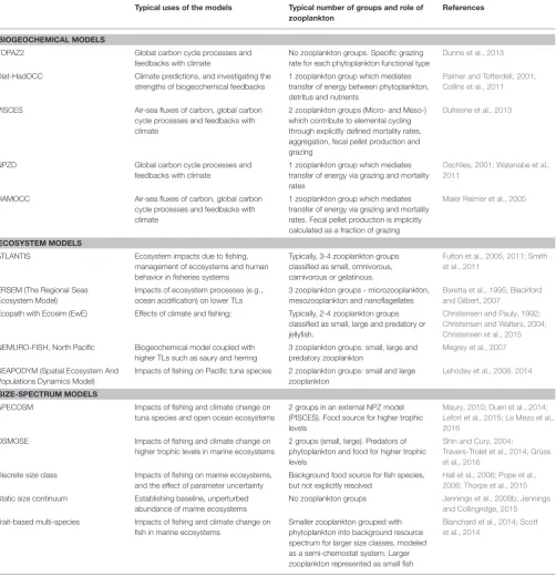
TABLE 1 | A list of common biogeochemical, ecosystem and size-based models and how they represent zooplankton groups. Typical uses of the models Typical number of groups and role of
zooplankton
References
BIOGEOCHEMICAL MODELS
TOPAZ2 Global carbon cycle processes and feedbacks with climate
No zooplankton groups. Specific grazing rate for each phytoplankton functional type
Dunne et al., 2013
Diat-HadOCC Climate predictions, and investigating the strengths of biogeochemical feedbacks
1 zooplankton group which mediates transfer of energy between phytoplankton, detritus and nutrients
Palmer and Totterdell, 2001; Collins et al., 2011
PISCES Air-sea fluxes of carbon, global carbon cycle processes and feedbacks with climate
2 zooplankton groups (Micro- and Meso-) which contribute to elemental cycling through explicitly defined mortality rates, aggregation, fecal pellet production and grazing
Dufresne et al., 2013
NPZD Global carbon cycle processes and feedbacks with climate
1 zooplankton group which mediates transfer of energy via grazing and mortality rates
Oschlies, 2001; Watanabe et al., 2011
HAMOCC Air-sea fluxes of carbon, global carbon cycle processes and feedbacks with climate
1 zooplankton group which mediates transfer of energy via grazing and mortality rates. Fecal pellet production is implicitly calculated as a fraction of grazing
Maier Reimer et al., 2005
ECOSYSTEM MODELS
ATLANTIS Ecosystem impacts due to fishing, management of ecosystems and human behavior in fisheries systems
Typically, 3-4 zooplankton groups classified as small, omnivorous, carnivorous or gelatinous.
Fulton et al., 2005, 2011; Smith et al., 2011
ERSEM (The Regional Seas Ecosystem Model)
Impacts of ecosystem processes (e.g., ocean acidification) on lower TLs
3 zooplankton groups - microzooplankton, mesozooplankton and nanoflagellates
Baretta et al., 1995; Blackford and Gilbert, 2007
Ecopath with Ecosim (EwE) Effects of climate and fishing; Typically, 2-4 zooplankton groups classified as small, large and predatory or jellyfish.
Christensen and Pauly, 1992; Christensen and Walters, 2004; Christensen et al., 2015
NEMURO-FISH, North Pacific Biogeochemical model coupled with higher TLs such as saury and herring
3 zooplankton groups: small, large and predatory zooplankton
Megrey et al., 2007
SEAPODYM (Spatial Ecosystem And Populations Dynamics Model)
Impacts of fishing on Pacific tuna species 2 zooplankton groups: small and large zooplankton
Lehodey et al., 2008, 2014
SIZE-SPECTRUM MODELS
APECOSM Impacts of fishing and climate change on tuna species and open ocean ecosystems
2 groups in an external NPZ model (PISCES). Food source for higher trophic levels
Maury, 2010; Dueri et al., 2014; Lefort et al., 2015; Le Mezo et al., 2016
OSMOSE Impacts of fishing and climate change on higher trophic levels in marine ecosystems
2 groups (small, large). Predators of phytoplankton and food for higher trophic levels
Shin and Cury, 2004;
Travers-Trolet et al., 2014; Grüss et al., 2016
Discrete size class Impacts of fishing on marine ecosystems, and the effect of parameter uncertainty
Background food source for fish species, but not explicitly resolved
Hall et al., 2006; Pope et al., 2006; Thorpe et al., 2015
Static size continuum Establishing baseline, unperturbed abundance of marine ecosystems
No zooplankton groups Jennings et al., 2008b; Jennings and Collingridge, 2015
Trait-based multi-species Impacts of fishing and climate change on fish in marine ecosystems
Smaller zooplankton grouped with phytoplankton into background resource spectrum for larger size classes, modeled as a semi-chemostat system. Larger zooplankton represented as small fish
Blanchard et al., 2014; Scott et al., 2014
The key references for each model is provided. The list is not intended to be an exhaustive list, but rather provide a starting point for those researchers interested in a particular modeling approach. For a more detailed list of models we point the reader toBopp et al. (2013)andArora et al. (2013).
nutrients held within the zooplankton back into the environment over time. Given this simple structure, it is arguable whether “zooplankton” included in some biogeochemical (lower trophic level) models can be considered to equate even conceptually with zooplankton in real systems. The “zooplankton” pool in these models must account for storage of all carbon and nutrients
that has been taken up from phytoplankton and detritus by grazing but not yet returned to the pool of detritus and available nutrients through respiration and mortality, i.e., the biomass of all animals in the system.
TABLE 2 | A list of some zooplankton data repositories whose data can be used for model assessment.
Program Region Availability
CPR
SAHFOS North Atlantic Available on request: http://www.sahfos.ac.uk Scientific Committee on Antarctic Research (SCAR) Southern Ocean Available on request: https://data.aad.gov.au Integrated Marine Observing System (IMOS) Australia Download from: https://portal.aodn.org.au
NETS
Bermuda-Atlantic Time-Series (BATS) Sargasso Sea Download from: http://bats.bios.edu California Cooperative Oceanic Fisheries Investigations (CalCOFI) California, U.S.A Download from: http://calcofi.org/data.html Census of Marine Zooplankton (CMarZ) Global repository Download from: http://www.cmarz.org/ Coastal and Oceanic Plankton Ecology, Production, and Observation
Database (COPEPOD)
Global repository Download from: http://www.st.nmfs.noaa.gov/copepod/ (Tools for data-analysis also available)
Hawaii Ocean Time-Series (HOTS) Oahu, Hawaii, U.S.A Download from: http://hahana.soest.hawaii.edu/hot/ Integrated Marine Observing System (IMOS) Australia Download from: https://portal.aodn.org.au Ocean Biogeographic Information System (OBIS) Global Repository Download from: http://beta.iobis.org Scientific Committee on Antarctic Research (SCAR) Southern Ocean Download from: https://data.aad.gov.au Western Channel Observatory (L4) W. English Channel Download from: http://www.bodc.ac.uk/
MARine Ecosystem DATa (MAREDAT) Global Repository Download from: http://www.pangaea.de/search?&q=maredat
BIOACOUSTICS
IMOS Australia Download from: https://portal.aodn.org.au National Centers for Environmental Information (NCEI) Global Download from: https://www.ngdc.noaa.gov Southern Ocean Network of Acoustics (SONA) Southern Ocean Download from: https://sona.aq
Please note there will be overlap in the data contained within some of these repositories.
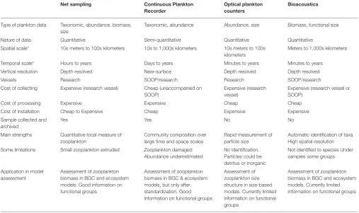
TABLE 3 | An overview of the resolution, data type and strengths and weaknesses of the four main observation platforms described in this manuscript. Net sampling Continuous Plankton
Recorder
Optical plankton counters
Bioacoustics
Type of plankton data Taxonomic, abundance, biomass, size
Taxonomic, abundance Abundance, size Biomass, functional size Nature of data Quantitative Semi-quantitative Quantitative Quantitative
Spatial scale* 10s meters to 100s kilometers 10s to 1,000s kilometers 10s meters to 100s kilometers
Meters to 1,000s kilometers Temporal scale* Hours to years Days to years Minutes to years Minutes to years
Vertical resolution Depth resolved Near-surface Depth resolved Depth resolved Vessels Research SOOP/research Research SOOP/research Cost of collecting Expensive (research vessel) Cheap (unaccompanied on
SOOP)
Expensive (research vessel)
Expensive (research vessel or SOOP)
Cost of processing Expensive Expensive Cheap Cheap Cost of installation Cheap to Expensive Cheap Expensive Expensive Sample collected and
archived
Yes Yes No No
Main strengths Quantitative local measure of zooplankton
Community composition over large time and space scales
Rapid measurement of particle size
Automatic identification of taxa High spatial resolution Some limitations Small zooplankton extruded Zooplankton damaged
Abundance underestimated
No identification. Particles could be detritus or inorganic
Not identified to species Under samples some groups Application in model
assessment
Assessment of zooplankton biomass in BGC and ecosystem models. Good information on functional groups
Assessment of zooplankton biomass in BGC & ecosystem models, but only after standardization. Good information on functional groups
Assessment of zooplankton size structure in size-based models. Currently limited information on functional groups
Assessment of zooplankton biomass in BGC and ecosystem models. Currently limited information on functional groups
zooplankton is represented as an all-encompassing mortality rate for phytoplankton (Christian et al., 2010; Dunne et al., 2013; Holzer and Primeau, 2013; Matear and Lenton, 2014). Instead of explicitly modeling the interaction between primary and secondary consumers, these models include a parameter that captures the consumption of phytoplankton. These kinds of scaling parameters are rarely determined experimentally but rather they are tuned during model development and assessment to produce realistic model outputs for the region and parameter set (e.g.,Holzer and Primeau, 2013).
Biological complexity can be increased within this simple NPZD structure to represent the lower trophic levels of marine ecosystems with various elemental cycles or to include multi-zooplankton compartments separated into different functional and/or size groups (Fennel and Neumann, 2004). The use of multiple phytoplankton functional groups based on physiology (Follows et al., 2007), taxonomy (Chan et al., 2002), or morphology (Kruk et al., 2010) is common, but the use of zooplankton functional groups is relatively less common. There are however some examples that distinguish zooplankton functional groups on the basis of grazing strategies and basal metabolism (Zhao et al., 2008) or feeding strategies, size and palatability to higher trophic levels (Sun et al., 2010). If we are to increase the complexity of zooplankton in a biogeochemical model, we not only need improved parameterization (Mitra, 2009), but also quantitative observations with which to help assess an expanded model that includes multiple zooplankton functional groups.
Ecosystem Models
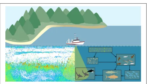
Ecosystem models attempt to describe the whole ecological system, from primary producers to higher trophic levels, often including human components (Figure 1B). Generally, these models have complex predator-prey interactions, including dozens to hundreds of species. Zooplankton however, are generally only represented by a few classes (e.g., Yool et al., 2011; Piroddi et al., 2015; Table 2), defined by diet (Pinnegar et al., 2005), functional type (Le Quere et al., 2005), or size (Griffiths et al., 2010; Ward et al., 2012; Savina et al., 2013; Watson et al., 2013; Pedersen et al., 2016), or a combination of these. Of course, some ecosystem models have many more zooplankton classes (e.g., Pavés et al., 2013). Despite these exceptions, research using common ecosystem modeling approaches— ECOPATH with ECOSIM (Christensen and Walters, 2004), ATLANTIS (Fulton et al., 2005), ERSEM (Baretta et al., 1995), and SEAPODYM (Lehodey et al., 2008)—tend to focus on fish and fisheries (Griffiths et al., 2010) and are hindered by uncertainties in the prey and predator relationships of zooplankton (Mitra and Flynn, 2006). Of course, models (of any kind) do not need to represent every detail of the environment to be useful or address a specific question (Fulton et al., 2003), however we do know that zooplankton is essential to understanding the transfer of energy to fish and fisheries (Friedland et al., 2012; Lassalle et al., 2013), and therefore care needs to be taken in the representation of this link between the lower and upper tropic levels (Rose et al., 2010; Shin et al., 2010).
The simplification of zooplankton groups in ecosystem models, while not always ideal, enables operationalization of the model, however understanding the effects of climate variability and change on the target species or fisheries (for example), can only be understood if the trophic pathways leading to them are well-defined. A common problem with how zooplankton are represented in both ecosystem and biogeochemical models is the false assumption that the same zooplankton assemblage is present throughout the whole domain, both horizontally and vertically, and the structure of this assembly does not change over time (Ward et al., 2014). These models lump multiple zooplankton functional groups together and use an “average” set of parameter estimates. Zooplankton assemblages change markedly in character from eutrophic systems, dominated by the classic short food chains and larger species, to oligotrophic systems, dominated by longer food chains and smaller species. They differ vertically, with predatory and larger species below the euphotic zone and are further complicated due to the complexity of zooplankton behavior and life-cycle strategies such as molting and diapause. These changes, which fundamentally affect nutrient cycles and fisheries production, are often poorly represented in models.
Size-Based Models
The size-based approach to marine ecosystem modeling (Figure 1C) has developed as an alternative to more traditional taxonomy-based frameworks by simplifying the community structure through classifying individuals based on size as opposed to species identity (Figure 1C; Sheldon and Parsons, 1967; Sheldon et al., 1972; Andersen and Beyer, 2015; Andersen et al., 2016). Developed over the past 50 years, this approach is based on empirical observations that individual and community processes such as growth, respiration, and predator-prey relationships and trophic position all scale with body size (Peters, 1983; Jennings et al., 2001; Brown et al., 2004; Andersen et al., 2016). Size-based modeling has two main approaches: (1) static size spectra models (Trebilco et al., 2013) and (2) dynamic size spectra models (Blanchard et al., 2017). Similar to the trophic food web structuring ofLindeman (1942), discrete size spectrum models (or macroecological models) aggregate individual organisms into discrete trophic levels based on size (Jennings and Mackinson, 2003; Jennings et al., 2008a). In comparison, dynamic size spectrum models add the element of time, and scale individual size-based growth and mortality rates to the population and community level (Benoit and Rochet, 2004; Blanchard et al., 2009; Hartvig et al., 2011; Jacobsen et al., 2013; Maury and Poggiale, 2013; Dueri et al., 2014; Guiet et al., 2016).
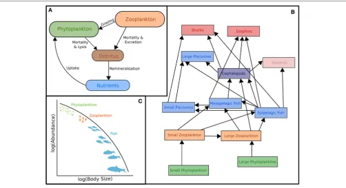
FIGURE 1 | Representation of typical models featuring zooplankton: (A)Biogeochemical (NPZD or LTL) models,(B)Ecosystem models (HTL) and(C)
Size-spectra models. Although not shown, all these models have temporal and spatial components. Individual-Based Models are not included in this schematic because they have many different forms which cover(A–C). For more information on IBMs see Section Individual Based Models and references therein.
of biomass and production at higher tropic levels in these models (Jennings and Collingridge, 2015).
Those models that have focused on zooplankton dynamics and food web structure explicitly resolve size-based zooplankton dynamics (Zhou and Huntley, 1997; Zhou, 2006; Baird and Suthers, 2007, 2010; Zhou et al., 2010), but do not explicitly include fish. To date, there have been few attempts to link these size-based zooplankton models to dynamic size spectrum models that have focused on higher trophic levels (but see OSMOSE;Shin and Cury, 2004). With increasing emphasis on understanding ecosystem impacts of climate variability and change, comes the need to better model bottom-up processes and thus the representation of zooplankton.
Individual Based Models
Individual based models (IBM) simulate individual animals, or groups of individuals as “superorganisms” that are treated as individuals. This allows a sophisticated representation of the behavior and/or physiology of each animal. For instance, IBMs can be structured so that they simulate the movements of animals in response to local light conditions (Batchelder et al., 2002), predator/prey encounters (Gerritsen and Strickler, 1977), or other environmental cues (Batchelder et al., 2002). In the planktonic environment, the main advantage of using an IBM is to account for rare individuals, circumstances or behaviors that contribute strongly to determining the overall population structure or variability; these are difficult to include in a state-variable approach (Werner et al., 2001). Rice et al. (1993), for
example, show how variability in larval growth and survival rates can mean that the characteristics of a population of zooplankton can be quite different from the mean characteristics of the individuals within that population.
By simulating individual organisms, IBMs replicate the stochastic variability in the nutritional status, life-cycle stage, or behavior that exists within a population and that may have emergent implications for the overall properties of that population. These include modeling the variability in the survival of larval fish (Letcher et al., 1996), investigating implications of nutrition and reproductive status for food web dynamics of
Breckling et al. (2006)provide a more general discussion of the use of IBMs in ecological theory.
ZOOPLANKTON SAMPLING SYSTEMS
FOR MODEL ASSESSMENT
Before we discuss approaches to integrate zooplankton observations and models, we will briefly describe the major zooplankton sampling systems used for collecting zooplankton observations (Table 3), the different types of data each produces, and the characteristic temporal and spatial sampling scale, which includes the sampling extent, interval, and grain size (resolution).
There is no single best way to sample zooplankton. In the treatise by Wiebe and Benfield (2003), essential reading for observationalists and modelers, they describe 164 different zooplankton sampling systems, ranging from nets to optical sensors. This staggering variety of systems, each with distinct sampling characteristics, has evolved to answer specific zooplankton research questions, not for ease of uptake into models. Here we discuss four major types of zooplankton sampling systems that have been used in model assessment: nets; the CPR; size-based systems (e.g., OPC/LOPC and ZooScan); and bioacoustics (seeTable 3).
Net Sampling
The use of nets is the oldest and most common method of sampling zooplankton. The recent history of zooplankton net sampling dates back to Thompson in 1828 (Wiebe and Benfield, 2003), but there are recorded observations prior to this (e.g., Sir Joseph Banks on the Endeavor in 1770; Baird et al., 2011). There are many different net configurations in use, but the key attributes that influence model assessment are the monitoring design, sampling characteristics, and the information derived from samples.
Sampling Characteristics
The large spatial and temporal extents of net sampling programs make their data well-suited for model assessment. Nets are used to collect zooplankton over a broad range of temporal extents—from hours to decades—and horizontal and vertical sampling grain sizes—from 10s of meters to 100s of kilometers (Table 3). The scale of a particular data set is usually dependent upon the aim of the survey. Process cruises tend to be one-off and are usually less useful for model assessment, unless the research cruise was specifically designed to answer a question that the model is addressing. Typically, data collected from long-term monitoring programs are more useful. Most monitoring programs involve point sampling, sampling weekly or monthly over many years. There are also many larger-scale surveys, often linked with fisheries assessments, that are collected seasonally or annually (e.g., CalCOFI:Edwards et al., 2010; or SARDI:Ward and Staunton-Smith, 2002).
There are four main characteristics to consider when using zooplankton data for model evaluation: type of tow, depth (and vertical resolution) of sampling, time of day, and mesh size. In terms of type of tow, nets can be dragged vertically, obliquely or more or less horizontally at specific depths (depth-stratified by
an opening-closing net). All three types of net tows are good for sampling mesozooplankton (0.2–20 mm), although oblique and depth-stratified tows are better for capturing macrozooplankton (2–20 cm), as the net often has a larger mouth area and is towed faster, providing less opportunity for zooplankton to escape. Conversely, faster tow-speeds can result in increased extrusion of smaller individuals. Net avoidance of macrozooplankton such as Antarctic Krill can be minimized with the use of strobe-lights (Wiebe et al., 2004) which are thought to either “dazzle” the plankton, or attract them. Nets are typically towed in the mixed layer (top 50–100 m) or from near the seafloor to the surface. Nets that sample in the mixed layer during the day typically underestimate zooplankton abundance and biomass because larger zooplankton often vertically migrate out of the mixed layer during the day; thus, higher biomass is typically found during the night.
Mesh size is probably the most important net characteristic and varies depending on the size of the target group of zooplankton and the ecosystem of interest. Macrozooplankton are usually sampled with a larger mesh size—500 µm, for example, is commonly used for fish larvae. Historically, many researchers have used 330 µm mesh for mesozooplankton (Moriarty and O’Brien, 2013), but a finer mesh of 200 µm is now almost universally used in temperate and polar systems to better sample smaller zooplankton (Sameoto et al., 2000). However, fine mesh nets (100µm) more quantitatively capture the smaller part of the mesozooplankton and some of the larger microzooplankton (e.g., juvenile stages of small copepods). Fine mesh nets are most commonly used in tropical areas where the zooplankton are generally smaller. Although coarse mesh nets extrude smaller zooplankton and thus underestimate abundance and biomass (Box 1), they still capture large organisms reasonably well (Sameoto et al., 2000).
Information Derived from Net Samples
For model assessment, probably the simplest and most useful information derived from net samples is zooplankton biomass. Biomass is measured in several different ways: settled volume, displacement volume, wet weight, dry weight, or occasionally carbon (Postel et al., 2000). Each is measured on different scales, and can be converted from one to another using standard conversions (Box 1). Occasionally, samples are poured through meshes of several different sizes and then weighed, providing biomass in different size categories (Huo et al., 2012; Banaru et al., 2014). Other information available from net samples is typically some idea of the zooplankton community present. This can vary from a coarse identification of the community (e.g., copepods, chaetognaths, jellyfish) to species-level identification. Taxonomic identification allows for use in IBM, or the subsequent aggregation of data into functional groups that might be represented in ecosystem models (e.g., mesozooplankton, herbivores, calcifiers).
The Continuous Plankton Recorder
BOX 1 | DATA WRANGLING: CONVERTING ZOOPLANKTON BIOMASS BETWEEN DIFFERENT UNITS.
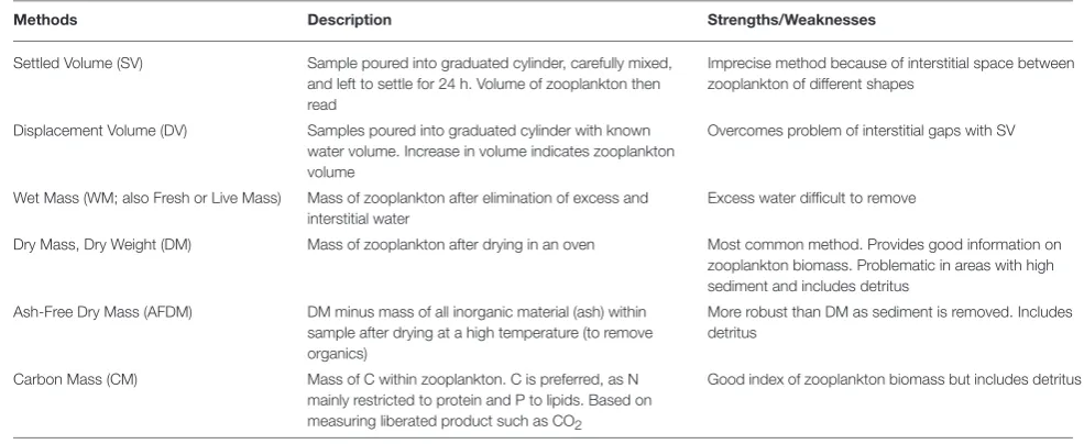
Model assessment using zooplankton biomass is not as straightforward as it might seem because observationalists use a range of different measures, from volumetric to elemental measures, of zooplankton biomass.Table B1briefly outlines the different units used to measure zooplankton biomass; for detailed information on the various methods seePostel et al. (2000). These different measures of zooplankton biomass all have their different strengths and weaknesses. We have ordered the rows ofTable B1by the robustness of the different methods and the ease in which they can be used in modeling, ranging from the most imprecise (Settled Volume) to the most robust (Carbon Mass).
[image:8.595.48.541.188.390.2]Most models usually use a currency of Nitrogen (or sometimes Carbon) biomass, which is rarely measured.Table B2provides a series of equations to convert different biomass to Carbon Mass. Once estimates are in Carbon Mass, they can be converted to Nitrogen Mass by using the C:N ratio of zooplankton, which typically varies from 4:1 to 6:1, but is commonly 5:1 (Postel et al., 2000).
TABLE B1 | Glossary of zooplankton biomass terms, and their strengths/weaknesses.
Methods Description Strengths/Weaknesses
Settled Volume (SV) Sample poured into graduated cylinder, carefully mixed, and left to settle for 24 h. Volume of zooplankton then read
Imprecise method because of interstitial space between zooplankton of different shapes
Displacement Volume (DV) Samples poured into graduated cylinder with known water volume. Increase in volume indicates zooplankton volume
Overcomes problem of interstitial gaps with SV
Wet Mass (WM; also Fresh or Live Mass) Mass of zooplankton after elimination of excess and interstitial water
Excess water difficult to remove
Dry Mass, Dry Weight (DM) Mass of zooplankton after drying in an oven Most common method. Provides good information on zooplankton biomass. Problematic in areas with high sediment and includes detritus
Ash-Free Dry Mass (AFDM) DM minus mass of all inorganic material (ash) within sample after drying at a high temperature (to remove organics)
More robust than DM as sediment is removed. Includes detritus
Carbon Mass (CM) Mass of C within zooplankton. C is preferred, as N mainly restricted to protein and P to lipids. Based on measuring liberated product such as CO2
Good index of zooplankton biomass but includes detritus
TABLE B2 | Equations to convert different biomass methods to carbon mass, Rearranged fromPostel et al. (2000).
Conversion Equation References
SV to DM log10(DM)=1.15∗log10(SV)−2.292 Postel, 1990
DV to CM log10(CM)=(log10(DV)+1.434)/0.820 Wiebe, 1988
WM to CM log10(CM)=(log10(WM)+1.537)/0.852 Wiebe, 1988
DM to CM log10(CM)=(log10(DM)+0.499)/0.991 Wiebe, 1988
AFDM to CM log10(CM)=(log10(AFDM)−0.410)/0.963 Bode et al., 1998
and in southern Africa. Unlike nets, there is only one main CPR design that has remained relatively unchanged over the years (Reid et al., 2003). Key attributes of the CPR that influence model assessment are monitoring design, its sampling characteristics, and the information derived from the samples (Richardson et al., 2006).
Sampling Characteristics
The large spatial and temporal extents characteristic of CPR surveys make the data well-suited for model assessment. The CPR collects zooplankton over greater time and space scales than net sampling—from days to decades and from 10s of kilometers to 1,000s of kilometers (Table 3). The temporal grain size (duration of a transect segment) is 15–30 min and the sampling interval between transects is typically a month or longer. The horizontal resolution (length of a transect segment) is 10–20 km. The CPR is not used for short-term process studies, but is deployed routinely
by commercial vessels plying common shipping routes, making it ideal for studying trends over time (Richardson et al., 2006).
The CPR is towed near-surface (∼7 m), but the draft of the large towing vessels probably mixes water down to 15 m. The aperture of the CPR is small (1.27 × 1.27 cm) and prevents large macrozooplankton such as jellyfish (scyphomedusae) from entering, although small and juvenile euphausiids are sampled (Hunt and Hosie, 2003). Fragile organisms, such as gelatinous plankton, are poorly sampled by the CPR because they are damaged when they come in contact with the silk mesh. For more detailed information about CPR sampling characteristics, seeRichardson et al. (2006).
[image:8.595.54.550.405.494.2]over space are robust (see Section Simple Observation Models: Simulated Sampling from a Model). Small zooplankton are likely to be under-sampled because of extrusion through the relatively large mesh size of silk used in the CPR (270µm) compared with standard nets (Sameoto et al., 2000). Large zooplankton are likely to be under-sampled by the CPR because of active avoidance (Clark et al., 2001; Hunt and Hosie, 2003; Richardson et al., 2004).
Notwithstanding the semi-quantitative nature of CPR sampling, it captures a roughly consistent fraction of thein situ
abundance of each taxon and thus reflects the major patterns observed in the plankton (Batten et al., 2003). Seasonal cycles estimated from CPR data for relatively abundant taxa are repeatable each year (Edwards and Richardson, 2004) and show good agreement with other samplers such as WP-2 nets (Clark et al., 2001; John et al., 2001) and the Longhurst Hardy Plankton Recorder (Richardson et al., 2004). Inter-annual changes in plankton abundance are also captured relatively well by the CPR (Clark et al., 2001; John et al., 2001; Melle et al., 2014) because the time-series has remained internally consistent, with few changes in the design of the CPR or in counting procedures.
Information Derived from CPR Samples
Data from the CPR are zooplankton abundance, with no direct estimate of biomass. Data are normally expressed in numbers per sample. Although each sample represents∼3 m3of filtered seawater, abundance estimates are seldom converted to per m3 estimates in practice because of their semi-quantitative nature.
As with net samples, a strength of CPR data is that taxonomic information is available. Typically, the copepods are well-resolved to species and the other groups to higher taxonomic levels (see Table 5 in (Richardson et al., 2006) for the taxa counted). This means that the data may be aggregated into functional groups that equate to those in models (e.g., Lewis et al., 2006). The CPR also retains phytoplankton (although not quantitatively) because of the leno silk weave of the mesh (see Richardson et al., 2006for details). Phytoplankton are counted to the lowest possible level using light microscopy and these data can be aggregated into phytoplankton functional groups that equate to those in models, such as diatoms and dinoflagellates, and used for model assessment alongside zooplankton data (e.g., Lewis et al., 2006).
Optical Plankton Counters
The most common instruments for measuringin-situsize spectra are the Optical Plankton Counter (Herman, 1988) and Laser Optical Plankton Counter (Herman, 2004). These instruments use either light emitting diodes-LEDs (LED-OPC) or lasers (LOPC) to measure the optical density and cross-sectional area of each particle as it passes through the sampling tunnel, and thereby estimate surface area (Sprules and Munawar, 1986; Suthers et al., 2006; Basedow et al., 2010). Hereafter we generalize, and refer collectively to both instruments as an OPC.
Sampling Characteristics
The large temporal and/or spatial extents and high temporal and spatial resolutions characteristic of OPC deployments make
the data well-suited for model assessment. The OPC collects information of the size-spectra of zooplankton over a broad range of temporal and spatial extents—from minutes to years and from 10s of meters to 100s of kilometers (Table 3). Due to the continuous electronic data collection of OPCs, there is no typical grain size (length of sample segment), and it depends largely on the purpose of the study and deployment method. OPCs can be deployed vertically (Vandromme et al., 2014; Marcolin et al., 2015; Wallis et al., 2016), mounted on a towed undulating vehicle to obtain high-resolution estimates of size spectra through space and time (Zhou et al., 2009; Everett et al., 2011; Basedow et al., 2014), mounted on a net frame (Herman and Harvey, 2006; Checkley et al., 2008; Marcolin et al., 2013), integrated with autonomous floats (Checkley et al., 2008), or mounted in the laboratory for the processing of net-samples (Moore and Suthers, 2006). OPCs are capable of sampling through the water column (up to 660 m deep) and if mounted on a towed body, over regional scales (100s km). OPCs are only deployable on research vessels for a range of reasons including: they need a trained technician to monitor them, require power via the tow-cable (or regular changing of data-logger batteries) and cannot be towed at the full speed of most commercial vessels. Therefore, unlike the CPR, they are not suited to ships of opportunity.
Taxonomic information is not directly available from OPCs, but they are often partnered with net samples, either by mounting within the net mouth (Herman, 2004) or as part of a broader sampling program whereby net and OPC samples are taken in close proximity to provide species-specific information, particularly for mono-cultures (e.g., overwintering
C. finmarchicus; Gaardsted et al., 2011 or swarms of Thalia democratica;Everett et al., 2011). As for all sampling techniques, gear avoidance and sampling volume can be a problem when zooplankton abundance is low (Basedow et al., 2013), due to the small aperture of the OPC (20–49 cm2) however these can be partially resolved by towing at a higher speed or for longer periods. Size-based data are also available from other instruments such as thein-situVideo Plankton Recorder (Davis et al., 2004) or the lab-based ZooScan (Vandromme et al., 2014 requires net samples). Inter-comparisons of size spectra between LOPC and ZooScan (Schultes and Lopes, 2009; Vandromme et al., 2014; Marcolin et al., 2015) or LOPC and VPR (Basedow et al., 2013) have shown mixed results. The biggest differences between ZooScan and the LOPC are thought to be due to the sampling of sediment in the small size-classes by the LOPC in coastal areas (Schultes and Lopes, 2009), although techniques have been developed to account for this (Jackson and Checkley, 2011) and can result in improved correlations between LOPC and ZooScan (Marcolin et al., 2015).
Information Derived from OPC
1978). The NBSS is a histogram-style size-distribution, in which the biovolume (or biomass) in a size class is normalized by the width of the size-class, such that the normalized distribution is independent of the width of size-classes (Platt and Denman, 1977). Using size-spectra theory, it is possible to extract trophic level and growth and mortality rates from in-situ OPC data (Edvardsen et al., 2002; Zhou, 2006; Basedow et al., 2014).
Other Optical Instruments
While OPCs are the most commonin-situoptical instruments, the field is developing rapidly and there are a range of other systems which deserve to be mentioned. In particular, camera and imaging systems such as ZooScan (Laboratory only; Grosjean et al., 2004), FlowCam (Laboratory only;Sieracki et al., 1998), Zooplankton Visualization system (ZOOVIS;Trevorrow et al., 2005), Video Plankton Recorder (VPR; Davis et al., 2005), Lightframe On-sight Keyspecies Investigation (LOKI; Schmid et al., 2016), and theIn SituIchthyoplankton Imaging System (ISIIS; Cowen and Guigand, 2008) have become more widespread. Additionally, increased effort has been invested in the identification of zooplankton from images (Zooniverse, www.planktonportal.org). The highly depth-resolved individual images from these systems provide detailed information on both taxonomy and individual features (e.g., proportion of females carrying egg sacs) which will be beneficial to model assessment of IBM’s. Moreover, developing artificial intelligence techniques (Layered neural networks, random forest algorithm and evolutionary algorithms) have permitted impressive advances in the automated detection of such features (Bi et al., 2015) and will add significant value to these optical systems.
Bioacoustics
Sampling Characteristics
Bioacoustic data can provide estimates of zooplankton and fish distribution, behavior and abundance using soundwaves and knowledge of the target strength of individual taxa (Foote and Stanton, 2000; Simmonds and MacLennan, 2005). Bioacoustic systems operate over fine to large scales, and are able to measure horizontal and vertical scales simultaneously (Table 3). Bioacoustic data for zooplankton can be obtained from single, multiple and broad band frequencies using ship-based systems or fixed platforms such as moorings (Godø et al., 2014). For mesozooplankton (∼0.2–20 mm) high frequencies are used from 100 KHz to 10 MHz in moored or profiling devices to resolve the size classes and types of organisms (Holliday et al., 2009). Acoustical backscatter from zooplankton are collected by the acoustic receiver and analyzed to estimate biomass or relative change in biomass of dominant scattering groups (Holliday and Pieper, 1995; Lavery et al., 2007; Kloser et al., 2009; Godø et al., 2014; Irigoien et al., 2014; Lehodey et al., 2014). The spatial resolution can be increased by moving the acoustic sensor, by using multiple spatially distributed sensors, or by tracking organisms within the acoustic beam (Godø et al., 2014). The temporal resolution of the backscatter can be improved by increasing the ping rates to resolve an individual’s distribution and behavior patterns (Holliday et al., 2009; Godø et al., 2014).
Bioacoustic techniques offer a number of advantages over traditional net or CPR sampling because they provide high-resolution data at both spatial (horizontal and vertical) and temporal scales depending on the deployment platform. High-frequency, broadband systems enhance the sampling resolution to millimeter scale so that smaller targets, such as copepods, can be quantified (Holliday et al., 2009; Godø et al., 2014). Where patches of plankton and fish are small (Benoit-Bird et al., 2013), plankton nets and the CPR do not provide an accurate picture of the spatial distribution of the organisms that they capture as the sampling volumes are far larger than the patches (Godø et al., 2014). In addition, bioacoustics can provide better biomass estimates when combined with other methods such as nets (Kaartvedt et al., 2012) as there are minimal gear avoidance problems.
Information Derived from Bioacoustics
Raw data from bioacoustics platforms is backscatter intensity over a single multiple or broad band of frequencies. A skilled analyst, using in isolation or a combination of scattering models, nets or optical sampling, is able to convert backscatter intensity to estimates of either biomass, abundance or (with more difficulty) broad taxa or potentially size groups (Holliday et al., 2009) depending on the region being considered. The high spatial and temporal resolution of these data are ideal for integration with modeling techniques. In the case of zooplankton, a major complicating factor in the use of multi-frequency bio-acoustic techniques is the diversity of this community, where a wide range of organisms of different sizes, shapes, orientations, and material properties occur together in the water column (Holliday and Pieper, 1995; Lavery et al., 2007). All these characteristics, along with their behavior, influence the way in which they scatter sound. To estimate their individual acoustic reflectance or target strength (TS), a series of zooplankton sound scattering models have been developed (Table 1 fromLavery et al., 2007) to account for that diversity.
ZOOPLANKTON DATA IN MODEL
ASSESSMENT
The performance of the zooplankton component of numerical models is rarely assessed against field observations because, unlike other parameters such as temperature or chlorophyll a
challenge, we turn our focus to a discussion of the two primary ways to link zooplankton in models with zooplankton observations: (1) data wrangling that transforms observational data to be directly comparable with model outputs; and (2) observation models that transform model output to be more comparable with observational data.
Data Wrangling: Transforming
Observational Data to Be More Like Model
Outputs
Data wrangling is the process of iterative data exploration and transformation from one format to another to make them more useful (Kandel et al., 2011). We use the term here to describe the series of steps that transforms observational data into a form that is more comparable with model output. Data wrangling transforms observed data into model-ready datasets. Data wrangling takes many forms, but two of the most important are conversion of observed biomass into appropriate values to compare with model estimates (see Box 1 for details), and collating biomass estimates collected using nets with different mesh sizes or different sampling devices (seeBox 2for details).
One example of data wrangling is finding the optimal way to interpolate scattered observations onto a regular model grid at a fixed point in time (Buitenhuis et al., 2013; Moriarty and O’Brien, 2013). A more complex example is the conversion of observed zooplankton abundance (or biovolume) to nitrogen (or carbon) biomass, which is how many models represent zooplankton biomass (Box 1). This approach requires assumptions about the size distribution and stoichiometry of zooplankton in the sample. Given these assumptions, modelers are able to use these data, but need to understand the basis of the assumptions that are made, and the magnitude of the error inherent in the conversion.
Often gridded data products—think of the global chlorophyll
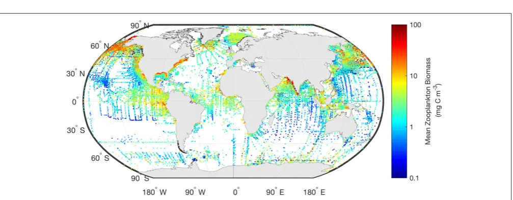
aproducts—are the most readily used for model assessment of phytoplankton. Similarly, the wrangling of 153,163 zooplankton biomass values, from a variety of locations, formats and collection methods, into a freely-available gridded global database of consistent biomass units was an amazing effort (COPEPOD; http://www.st.nmfs.noaa.gov/copepod/; Moriarty and O’Brien, 2013). Unlike chlorophyllahowever whose global satellite maps are updated daily, the time-consuming nature of zooplankton collection means there isn’t a truly global database (see gaps inFigure 2) which is updated on time-scales relevant to many modeling studies. These data are extremely useful however, to constrain model estimates by providing biomass limits against which to assess our models. There are many statistical tools available to assist with the practical side of data-wrangling (e.g., “tidyr” or “dplyr” in R), but the most important aspect is dialogue between modelers and observationalists.
Observation Models: Transforming Model
Output So It Is More Like Observational
Data
Where zooplankton observations are incorporated into models, there is often a mismatch between the observations (often infrequent point measurements) and the high spatial and
temporal resolution of models. Observation models are one technique that can help address these mismatches, allowing model assessment at a range of scales. We define an observation model as a model that takes the output of a simulation and transforms it to a form that closely resembles the observations with which it is being compared. This approach of generating observations from models is used in numerical weather prediction (Dee et al., 2011), acoustic observations of mid-trophic levels (Handegard et al., 2012), and remotely-sensed ocean color observations (Baird et al., 2016).
The observation model needs to be based on sufficient process understanding, so that it applies well over a broad range of environments and the error in the output of the observation model is due primarily to the simulation model estimate (i.e., zooplankton biomass) and not the accuracy of the parameters or equations within the observation model itself. Essentially, the rationale of an observation model is to allow comparison of observed and modeled data, by removing inconsistencies in the structure or scale of these data. Here we review some of the steps and challenges to developing zooplankton observation models, for improved interpretation of the observations and assessment of numerical models. Below we discuss the range of observation models, from simple to more complex.
Simple Observation Models: Simulated Sampling from a Model
The simplest approach to developing an observation model is to undertake simulated sampling within a model, and compare these sampled data to zooplankton observations. For example, zooplankton biomass estimates can be extracted from a simulation corresponding to the time, location, and depth of the samples collected by nets, CPR, OPC, or bioacoustics. While not directly comparing their model to observations,Wiebe and Holland (1968)were likely the first to simulate net tows within a computer simulation when they determined the effect of net size and patchiness on sampling error.
BOX 2 | DATA WRANGLING: CONVERTING ZOOPLANKTON BIOMASS BETWEEN DIFFERENT MESH SIZES AND USING PROXY ESTIMATES Different mesh sizes:Different mesh sizes of nets provide very different biomass values, with higher zooplankton biomass estimates from finer mesh nets. To convert biomass data collected with different mesh sizes to an equivalent mesh size, common conversions can be applied (Table B3;Moriarty and O’Brien, 2013), although it must be acknowledged that the best conversion is dependent upon the zooplankton assemblage present. Fortunately, different net systems produce similar estimates of zooplankton when operated with similar mesh sizes (Skjoldal et al., 2013).
TABLE B3 | Equivalent mesh size conversions (modified fromMoriarty and O’Brien, 2013).
Conversion Equation References
333µm to 200µm mesh log10(CM200)=1.4461∗log10(CM333) O’Brien, 2005
505µm to 330µm mesh log10(CM333)=1.2107∗log10(CM505) O’Brien, 2005
Proxy estimates—Abundance:Sometimes zooplankton abundance and not biomass is measured. It is difficult to convert abundance to biomass because you do not know the size of individuals and thus their mass. In this situation, we recommend using abundance data for relative patterns—for example seasonal cycles, spatial variation, or inter-annual variation.Lewis et al. (2006)assessed their ecosystem model by normalizing both the model biomass and the observed abundance data and comparing the normalized patterns spatially and temporally.
Proxy estimates—Biovolume:Size-based methods of measuring zooplankton (LOPC/OPC/VPR/ZooScan) can provide estimates of zooplankton biomass. These instruments measure organism size (2-D area) and this can be converted to organism volume. Biovolume can then be converted to biomass by summing organism volume across all individuals and assuming zooplankton has the same density of seawater. Zooplankton biomass from the VPR and ZooScan has the advantage that detritus and sediment can be removed. An advantage of these size-based methods are that they can be used to estimate biomass in size classes. They could also be used to partition observed zooplankton total biomass into size classes (i.e., using the size spectra to estimate the % of biomass in different size classes and applying this to measured biomass).
FIGURE 2 | The mean marine zooplankton biomass (mg C m−3) for mesozooplankton (0–200 m depth) is shown illustrating the distribution of records from the most comprehensive database available.The data shown here are freely available from “COPEPOD: The Global Plankton Database”
(http://www.st.nmfs.noaa.gov/copepod/).
patterns in phytoplankton seasonality (e.g., spring diatom bloom in the model is too early), allowing the reparametrizing of the model (Lewis et al., 2006).
More Complex Observation Models: Add-On Models That Convert Output to Observations
With improving technologies and computing power comes the opportunity to embrace increasingly complex observation models. Here we borrow many examples from state-of-the-art applications in other fields of model assessment that have not yet been fully applied to zooplankton. These are ideally suited for the assessment of zooplankton models due to the inherent disconnect
between the spatial and temporal resolution and model currency of observations and models.
[image:12.595.48.552.320.516.2]FIGURE 3 | Sampling the model—(A)Simulated “tows” within the model were performed by extracting biomass data of omnivorous mesozooplankton from the exact time (day and nearest hour), location (longitude and latitude), and depth (7 m) of corresponding samples collected by the CPR.(B)The data are then standardized due to the different units, and the difference between normalized z -scores for both simulation and observation between January 1988 and December 1989 with a 3-day running mean (solid line) is shown. Black is model data, red is CPR data; dots are individual model tow points, crosses are individual CPR tow points (redrawn fromLewis et al., 2006).
FIGURE 4 | A bioacoustic observation model would apply the same scattering models to both the backscatter measurements from the ocean and the ecosystem model.Regardless of environment (ocean or model), we can use the same principle of the scattering models to produce echograms which can be directly compared.
the model, against satellite-derived water-leaving irradiance. The water-leaving irradiances, from the observation model and the satellite, can be directly compared against each other to assess the model. Alternatively, the water-leaving irradiance measures from both the observation model and the satellite, can be converted to chlorophyll a using one of the satellite algorithms in order to allow a comparison which may be more informative for those used to thinking about chlorophyll a. In either case, both the units of assessment, and the method used to derive them, are the same. Thus, the mismatch between simulated and observed remote-sensing reflectance provides an excellent metric for model assessment of the coupled biogeochemical model (Baird et al., 2016; Jones et al., 2016).
This approach—of building an observation model that enables the model to produce information more comparable to observations—has not yet been applied to zooplankton but would be a valuable way forward. For zooplankton model assessment, building observation models for size-spectra models would be fairly straightforward given that observational techniques (OPC, ZooScan and VPR) measure the size and abundance of the zooplankton community—metrics easily extracted from size-spectra models. It is also made easier because size size-spectra are typically represented as Normalized Biomass Size Spectra (NBSS; Section Optical Plankton Counters), where size classes are normalized by the width of the size-class, making the shape of the spectrum independent of the size-classes chosen (Platt and Denman, 1977). The NBSS can thus be generated from both the observations and models, even if they each have different resolutions. In addition to comparing state-variables, the size-based approach developed byZhou (2006),Zhou et al. (2010) provides an intuitive framework for estimating time-averaged rates (e.g., growth, mortality) for zooplankton from observed NBSS, which could then be tested within dynamic size spectrum models that include zooplankton (Heneghan et al., 2016) or compared to observed rates in the field (Zhou et al., 2010).
[image:13.595.45.291.333.474.2]and model outputs to a common format introduces error and inconsistencies into each. An alternative approach is to create a bioacoustic observation model which uses scattering models to estimate the backscatter intensity of zooplankton within the ecosystem model and compare this to bioacoustic observations in the ocean (Figure 4;Handegard et al., 2012). The main challenge for the observation model is to simulate the observed backscatter at a particular frequency and depth within the model. In this case, we are not directly modeling sound within the ecosystem model, so this observation model does not provide feedback (external forcings or changes in state variables) to the ecosystem model. It is simply about avoiding inconsistencies in the comparison of modeled and observed data, and enabling the comparison of “like with like.” Building such an acoustic observation model would simulate acoustic observations, producing an echogram (Figure 4). Thus, for all model points in time and space, the observation model could produce an echogram based on the zooplankton functional groups predicted by the ecosystem model. As with all model-observation comparisons, care must be taken to consider the temporal and spatial resolution measured or modeled. In the case of bioacoustics, the measurements will often be at a higher spatial resolution (meters;Table 3), but lower temporal resolution (minutes; Table 3) than the model. High-resolution bioacoustic measurements of abundance and biomass can be downscaled to match the resolution of ecosystem models. Clean acoustic observations will need to be readily available for comparison with the simulated outputs of the observation model, which could be achieved with the use of a multi-frequency acoustic mooring, which delivers acoustic data resolved vertically and temporally at a single site (Urmy et al., 2012).
CONCLUDING REMARKS
In this review, we summarize many of the fundamentals of zooplankton modeling for observationalists and zooplankton observations for modelers. As highlighted byFlynn (2005), we believe that there needs to be greater discussion and collaboration between modelers and observationalists. Only through dialogue will we be able to perform the data wrangling and develop
the observation models that are needed so our observations and model outputs align. In particular, observation models have not been applied in the assessment of zooplankton in models and are likely to be a powerful approach, as they have been in other disciplines. These observation models range from the simple (sampling the model) to the more complex (bioacoustics) and can even result in the underlying model being changed to output data that is directly comparable to the observations (e.g., water leaving irradiance and chlorophyll a). The development and use of complex observing models can be time consuming, but many of the techniques described above are already being implemented (Handegard et al., 2012; Baird et al., 2016). The adoption of these ideas for use in zooplankton research would be a major step forward, allowing zooplankton observations to be more readily used in model assessment as real-time data becomes a possibility with optical and acoustic systems. Here we have provided a few ideas. We hope that this review will increase the dialogue between modelers and observationalists, and provide the impetus for greater model assessment of zooplankton output through data wrangling and state-of-the-art observation models.
AUTHOR CONTRIBUTIONS
JE, AR, and MB conceived the original idea for this workshop and manuscript. All authors contributed to the writing of the manuscript. JE and AR wrote the final draft.
ACKNOWLEDGMENTS
This manuscript was written as part of the Integrated Marine Observing System (IMOS) “Zooplankton Ocean Observing and Modelling” workshop held in Hobart 15–16 February 2016. The workshop was funded by IMOS. JE was funded by an Australian Research Council Discovery Grant (DP150102656). The CPR and fauna images in Figures 1, 4, and 5 were provided by the Integration and Application Network, University of Maryland Center for Environmental Science (ian.umces.edu/imagelibrary/).
REFERENCES
Andersen, K. H., and Beyer, J. E. (2015). Size structure, not metabolic scaling rules, determines fisheries reference points.Fish Fish.16, 1–22. doi: 10.1111/faf. 12042
Andersen, K. H., Berge, T., Gonçalves, R. J., Hartvig, M., Heuschele, J., Hylander, S., et al. (2016). Characteristic sizes of life in the oceans, from bacteria to whales. Annu. Rev. Mar. Sci.8, 217–241. doi: 10.1146/annurev-marine-122414-034144 Arhonditsis, G. B., and Brett, M. T. (2004). Evaluation of the current state of mechanistic aquatic biogeochemical modeling.Mar. Ecol. Prog. Ser.271, 13–26. doi: 10.3354/meps271013
Ariza, A., Garijo, J. C., Landeira, J. M., Bordes, F., and Hernandez-Leon, S. (2015). Migrant biomass and respiratory carbon flux by zooplankton and micronekton in the subtropical northeast Atlantic Ocean (Canary Islands).Prog. Oceanogr. 134, 330–342. doi: 10.1016/j.pocean.2015.03.003
Arora, V. K., Boer, G. J., Friedlingstein, P., Eby, M., Jones, C. D., Christian, J. R., et al. (2013). Carbon–concentration and carbon–climate feedbacks in CMIP5 earth system models.J. Clim.26, 5289–5314. doi: 10.1175/JCLI-D-12-00494.1
Baird, M. E., and Suthers, I. M. (2007). A size-resolved pelagic ecosystem model. Ecol. Modell.203, 185–203. doi: 10.1016/j.ecolmodel.2006.11.025
Baird, M. E., and Suthers, I. M. (2010). Increasing model structural complexity inhibits the growth of initial condition errors.Ecol. Complexity7, 478–486. doi: 10.1016/j.ecocom.2009.12.001
Baird, M. E., Cherukuru, N., Jones, E., Margvelashvili, N., Mongin, M., Oubelkheir, K., et al. (2016). Remote-sensing reflectance and true colour produced by a coupled hydrodynamic, optical, sediment, biogeochemical model of the Great Barrier Reef, Australia: comparison with satellite data.Environ. Modell. Softw. 78, 79–96. doi: 10.1016/j.envsoft.2015.11.025
Baird, M. E., Everett, J. D., and Suthers, I. M. (2011). Analysis of southeast Australian zooplankton observations of 1938–42 using synoptic oceanographic conditions. Deep Sea Res. Part II Top. Stud. Oceanogr. 58, 699–711. doi: 10.1016/j.dsr2.2010.06.002