Multi frequency matching, classification, and cosmic evolution of radio galaxy populations

(1)

(2)

(3)

Multi-frequency

Matching,

Classiﬁcation,

and

Cosmic

Evolution

of

Radio

Galaxy

Populations

By

Jesse

Allen

Swan

BachelorofSciencewithFirstClassHonours

UniversityofTasmania,2013

AThesissubmittedinpartialsatisfaction oftherequirementsforthedegreeof

DoctorofPhilosophy in

Astrophysics inthe

SchoolofNaturalSciences ofthe

UniversityofTasmania Hobart,Australia

SupervisingComittee: DoctorStanislavShabala

ProfessorRayNorris AssociateProfessorAndrewCole

(4)

(5)

Declaration

This thesis contains no material which has been accepted for a degree or diploma by the Univer-sity or any other institution, except by way of background information and duly acknowledged in this thesis, and to the best of the my knowledge and belief no material previously published or written by another person except where due acknowledgment is made in the text of the the-sis.

Signed:

Jesse Allen Swan

(6)

(7)

Multi-frequency Matching, Classiﬁcation, and Cosmic

Evolution of Radio Galaxy Populations

Abstract

This thesis combines the third data release of the Australia Telescope Large Area Survey (AT-LAS) with complimentary DES photometry and OzDES targeted spectroscopy. ATLAS 1.4 GHz is a deep (< 20μJy/beam) survey of the combined 6.3 deg2sky area of CDFS and ELAIS-S1.

Cross-matching of 4903 ATLAS sources to photometric and spectroscopic counterparts is performed visually using custom interactive software: MCVCM. I compare the results from this visual matching to results from simple coordinate-based nearest-neighbour matching. The visu-ally constructed catalogues are substantivisu-ally more robust due to a better accounting of chance alignments and dense ﬁeld mismatches. Both cross-matching techniques are performed directly from radio-to-optical, and indirectly by matching radio sources to an infrared-optical paired catalogue. There is a deﬁnite improvement for both visual and nearest-neighbour cross-matching when performed via SWIRE infrared intermediary catalogue. I use the visual catalogue to build a reliable sample of ATLAS sources matched to SWIRE infrared photometry, DES optical photom-etry, and OzDES spectra. This catalogue was developed carefully and is intended to for use as a comparison and training catalogue for the development of intelligent automated cross-matching algorithms

(8)

(9)

to a young boy dreaming of exploring space

to a young boy dreaming of punching fighter jets through clouds a young boy dreaming of swords and magic and secret places dreaming of buying his mum and dad a new house

to a young boy, full of angst, wishing there was more to his life

(10)

(11)

Acknowledgments

Visualisation and analyses throughout this thesis were produced using customPythonscripts. These scripts rely heavily on the pre-existing Python packages: numpy,matplotlib,scipy, as-tropy,astroml,iPython,&scikit-learn. Spectral line ﬁtting utilised Michele Cappellari’s Python implementation ofpPXF. Nearest-neighbour positional cross-matching of catalogues was conducted inTOPCAT. Full ﬁeld image mosaics used Caltech University’smontage.

This thesis was written entirely inSublime Textand compiled usingLaTeXTools. Almost all code was also written in Sublime Text with the eventual (albeit, far too late) switch to the much more feature-richPyCharm. Spelling mitsakes and grammatical, errors in this thesis were eradicated withGrammarly. Many hours were saved during the assembly of the bibliography by use of Michele Vallisneri’sCompu-salon ADS database scraper.

Advice and insights were provided by my supervisors: Doctor Stas Shabala, Professor Ray Norris, and Associate Professor Andrew Cole; as well as by ATLAS team members: Rob Sharp, Doctor Nicholas Seymour, and Doctor Amy Kimball. The insight provided by the anonymous examiners of this thesis were invaluable, as they provided the ﬁnal trimming required to click this piece of work smoothly into the inﬁnite academic jig-saw.

Programming advice was curated from questions and answers onStack-Overflow. The Au-thor would in particular like to thank Stack Overﬂow userImportanceOfBeingEarnestfor his seemingly inﬁnite knowledge and passion for helping others.

With the exceptions of the acknowledgements above: the writing of this thesis, the scientiﬁc results herein, and all supporting code required for analysis was conducted or produced solely by

me,The Author.

I am grateful for the ﬁnancial support provided by the Australian Postgraduate Award, and especially the scholarship provided by The Mathematics and Physics department under the Uni-versity Of Tasmania’s Elite Research Scholarship program.

(14)

Figures listing

1 Hubble galaxy classiﬁcation sequence . . . 3

2 Illustration of the Uniﬁed Model for AGN . . . 7

3 ATLAS 1.4 GHz continuum maps of CDFS and ELAIS-S1 . . . 10

1.1 Photometric completeness of DES photometry . . . 12

1.2 MCVCM examples of common causes for incorrect cross-matches . . . 15

1.3 MCVCM examples of incorrect multi-component sources . . . 16

1.4 MCVCM examples of blended radio components . . . 17

1.5 Nearest-Neighbour cross-matching radius (DES–OzDES) . . . 21

1.6 Nearest-Neighbour cross-matching radius (ATLAS–DES & ATLAS–SWIRE) . 23 1.7 Optical cutout across three tiles . . . 26

1.8 Overlap of ATLAS, DES, and SWIRE . . . 27

1.9 Comparison of separation distance for techniques and data-paths . . . 29

1.10 ATLASmG,mR,mI,mZspectroscopic completeness . . . 31

2.1 pPXF ﬁtting and spectrum for source 2940027955 . . . 37

2.2 Visual Classiﬁcation: Star-Forming and Unknown . . . 38

2.3 Visual Classiﬁcation: Ellipticals . . . 39

2.4 Visual Classiﬁcation: Emission Line AGN . . . 40

2.5 BPT: visual classiﬁcations . . . 41

2.6 Lamareille blue-diagram: visual classiﬁcation . . . 41

2.7 Lamareille blue-diagram: classiﬁcations from BPT . . . 42

2.8 Lamareille blue-diagram: Combined classiﬁcation . . . 44

2.9 BPT: Combined classiﬁcation . . . 44

2.10 S1.4vs.S24,3.6,4.5,5.8,8,0μm: combined classiﬁcation . . . . 45

2.11 S24,3.6,4.5,5.8,8.0μm{S1.4vs.logp1`zq: combined classiﬁcation . . . 46

2.12 S24μm{S1.4vs.logp1`zq: manual re-classiﬁcation . . . 46

2.13 ATLAS redshifts: star-forming galaxies and AGN . . . 47

3.1 Representation of a redshift limited volume . . . 51

3.2 Representation of a radio limited volume . . . 52

3.3 Reconstruction of BH12 RLF: examples of automatic binning . . . 54

3.4 ATLAS 1.4 GHz luminosity versus redshift . . . 55

(15)

3.6 ATLASmG,mR,mI,mZspectroscopic completeness . . . 57

3.7 Spectroscopic success rate ofG,R,I,Z . . . 58

3.8 ATLAS RLF of all sources: 0.005ăză0.26,0.26ăză0.58,0.58ăză1.0 60 3.9 ATLAS RLF of star-forming galaxies: ză0.26,0.26ăză0.58,0.58ăză1.0 63 3.10 ATLAS RLF of AGN:ză0.26,0.26ăză0.58,0.58ăză1.0 . . . 64

3.11 ATLAS RLF of unknown sources:ză0.26,0.26ăză0.58,0.58ăză1.0 . . 66

3.12 ATLAS RLF of unknown sources & AGN: 0.26ăză0.58,0.58ăză1.0 . . 67

3.13 High-zATLAS RLF of unknown sources & AGN:zą1.0 . . . 68

A.1 Examples of various states during an MCVCM cross-matching instance . . . . 80

B.1 Nearest-Neighbour cross-matching radius perturbation demonstration . . . 82

C.1 Recalculated ATLAS DR1 RLF . . . 83

C.2 MCVCM cutouts ofS24μmselected AGN (1–9 of 23) . . . 85

C.5 Spectra ofS24μmselected AGN (1–10 of 38) . . . 88

(16)

As we got farther and farther away, the Earth diminished in size. Finally, it shrank to the size of a marble, the most beautiful marble you can imagine … seeing this has to change a man

– James Irwin

0

Introduction

0.1 Galaxies

Edwin Hubble’s measurements of Cepheid variable stars in nearby dwarf galaxy NGC 6822 was the ﬁrst step in unfolding the true extent of our Universe (Hubble 1925). Before these re-sults, galaxies were thought to be nebulae within our small („ 300 000 light year diameter) ‘Universe of stars’; a Universe that we now know as the Milky Way Galaxy which is neither dis-tinct nor unique amongst a Universe of galaxies. Galaxies are vast quantities of gravitationally bound dust, gas, and stars embedded within a much larger dark matter halo (Navarro et al. 1996,1997). Most are host to a central super-massive black hole (SMBH) the mass of which is intimately tied to wider galactic properties.

0.1.1 Symptomatic Galaxy Classes

(17)

grav-ity as the gas cooled and collapsed stars began to form about local centres of mass, forming the ﬁrst galaxies. In these dense cosmic ﬁlaments, orbiting galaxies lost energy via dynamical friction merging into larger galaxies as the universe aged.

Separating these galaxies into classes is ubiquitously the first step in evaluating their prop-erties. As scientific instruments are advanced we are able to discover increasingly detailed dif-ference between galaxies within pre-defined classes, making classifications more complex and simultaneously improving our understanding of galaxy populations. The simplest and most obvious form of classification is via morphology, and the original and most famous of these is the Hubble Sequence (or colloquially, the Hubble Tuning Fork;Hubble 1936: see Figure 1). This classification scheme breaks galaxies into three classes: smooth and featureless ellipticals, spirals, and irregulars (a later addition to the scheme). Within each of these classes, there are subclasses that focus on elongation, or the presence of a spiral bar, for example.

The differences between morphologically selected galaxies provide an excellent basis for pop-ulation research. Spiral galaxies contain vast amounts of star formation, and their luminosity is dominated by these young, bright stars. They exist primarily in sparse clusters or cluster out-skirts˚_{and tend to have much smaller masses than elliptical galaxies. The more massive}

ellipti-cal galaxies have large featureless haloes and are dominated by an older stellar population due to a lack of ongoing star formation; they also tend to reside within denser cluster environments than spirals. Understanding the many differences between these galaxies and the environment that shapes them allows for the boot-strapping of more complex or controversial classiﬁcation schemes that serve even further to advance our understanding of galaxy formation and evolu-tion. Increasingly detailed observations and simulations of galaxies and galaxy populations fortify that understanding and allow new classiﬁcation schemes to be tested.

0.1.2 Modelling the Universe

Λ-CDM cosmology is the most broadly accepted cosmological model for the fundamental rea-son that it is thus far the best ﬁt to our observations of the Universe. Particularly the 2011 No-bel Prize for Physics was awarded to Adam Riess, Brian Schmidt, and Saul Perlmutter for their discovery of an accelerating expanding Universe (Riess et al. 1998;Perlmutter et al. 1999). The cosmological constantΛpredicts this accelerating expansion on the back of a cold dark matter (CDM) cosmological model. The CDM model estimates that roughly 5 per cent of energy is in the form of baryonic matter, 23 per cent is weakly interacting dark matter, and the remaining 72 per cent is dark energy permeating the entirety of space and accelerating the expansion of the Universe.

(18)

Figure 1:“Sequence of Nebular Types” (Hubble 1936, Figure 1). Hubble, E. states that mixed galaxy types exist between the two spiral branches and that the ‘S0’ transi on phase is hypothe cal. The transi ons between ellip cals are noted as smooth and con nuous.

Cosmological models such as these build upon over a century of observational data and help to advance astronomy by providing observational astronomy with a plethora of provably falsi-ﬁable predictions. These predictions act to focus astronomy and astrophysics on the furthering of our understanding of the Universe in signiﬁcant ways. Enormous galaxy surveys provide data on the low redshift Universe faster than current methodologies can process, and ground-breaking observational techniques coupled with incredible technology (such as adaptive optics and space telescopes) yield detailed information on some of the most distant objects in the uni-verse (e.g., gravitational lensed galaxies:Watson et al. 2015).

0.2 Radio Galaxies 0.2.1 A Radio Sky

(19)

allow-ing these sources to be detected at great distances with sallow-ingle dish telescopes and resolved with increasing detail using Long Baseline Arrays (LBA).

Bandpasses of radio-frequencies are sensitive to different physical processes. High-frequency radio is dominated by large-scale dust emission from thermal („ 20 K) gas in the disk of galax-ies (e.g., Planck 353 GHz sky map:Planck Collaboration et al. 2014a). Unfortunately, this means that extragalactic sources coincident with the galactic plane of our Milky Way (MW) suffer from dramatic line-of-sight extinction. For frequencies on the order of tens of gigahertz, the total sky-brightness is dominated by the Cosmic Microwave Background (CMB) colloqui-ally, ‘the after-glow of the Big Bang’, this light permeates all of space with a black body temper-ature of 2.73 K. Whilst the CMB broadly dominates the the Planck 30 GHz sky map (Planck Collaboration et al. 2014b), observations of galaxies in this frequency regime are dominated by thermal free-free emission, the tail of the 80 K galactic dust black-body spectrum, and syn-chrotron emission.

This thesis focuses primarily 1.4 GHz synchrotron radiation, decelerating electrons whose radiation can be approximated by a power lawFν9ναas they spiral along strong magnetic ﬁelds. These power-law spectra exhibit a break or turn-over due to (for example) free-free or synchrotron self-absorption (Jaffe & Perola 1973;O’Dea 1998). The observed ﬂux (for example) dominates the Haslam 408 MHz sky map (Haslam et al. 1982) but falls off rapidly at higher fre-quencies, the steepness of this decline being affected by a redshift and spectral ageing degener-acy (e.g.,Machalski et al. 2010, and references therein). Galaxies with sufficient star formation (SF) or those host to a bright active-galactic nucleus (AGN) are detectable at synchrotron radi-ation frequencies. In SF galaxies the synchrotron emission primarily originates from the accel-eration of electrons by supernova shocks, and (far less strongly) the free-free emission from Hii regions. In galaxies host to a powerful AGN the emission generated from powerful jets dwarfs that of the star-formation (P1.4ą1024W/Hz).

0.2.2 Understanding the Brightest Radio Galaxies

Early observations of radio galaxies revealed luminosities requiring energy inputs far beyond what is possible from star formation processes (Begelman et al. 1984). Even more puzzling was the rapid variability of the brightest of these sources (quasars) which could see 10 to 300 per cent changes in peak ﬂux over several days, or months (Smith & Hoffleit 1963;Greenstein & Schmidt 1964;Hunstead 1972). This variability provided the key for obtaining the spatial scale from which these vast emissions originated, restricted by the strict condition that the time-scale of luminosity variability is greater than the light-crossing time (i.e.,τvariability ą R{c;Mushotzky 1984).

(20)

Zel’dovich & Novikov(1964) in which they mathematically demonstrated that observed jets could be reproduced by the accretion of gas onto a supermassive black hole (SMBH) on the order of 106– 1010M@. This phenomenon would reproduce the energy output (with up to

10 per cent rest-mass energy conversion of in-falling gas) as well as the rapid variability due to the activity necessarily constrained to within tens to hundreds of Schwarzschild radii.

Supermassive black holes exist at the centre of most galaxies with the probability increas-ing as a function of galaxy mass (e.g.,Kormendy & Richstone 1995;Kormendy & Ho 2013). The Milky Way galaxy possesses a central SMBH (Sagittarius A*) with mass„ 4.1ˆ106M@

(Gillessen et al. 2009;Reid & Brunthaler 2004). The presence of Sagittarius A* has been inde-pendently conﬁrmed by multiple techniques: orbital periodicity of nuclear stars (Schödel et al. 2002;Gillessen et al. 2009); polarimetry (Bower et al. 1999;Meyer et al. 2006); Doppler mea-surements of orbiting dust and gas (Levin & Beloborodov 2003); water megamasers associated with the accretion disk (Miyoshi et al. 1995), and M–σvelocity dispersion relation (Ferrarese & Merritt 2000;Wyithe 2006). Sagittarius A* is not considered active, the search for jets has revealed only small remnants of previous activity (Doeleman et al. 2008;Bordoloi et al. 2017).

0.3 The Core of a Galaxy 0.3.1 Radio Jets

The mechanism for the production of radio jets took longer to establish than did the origin of the emission. In a 1971NaturepublicationRees(1971) ﬁrst posited that pressure of low-frequency (À 1 kHz) radiation:_{can produce a cavity within the central region, and if there}

is sufficient collimation of this radiation, jets of relativistic electrons are produced with high efficiency. This theory overcame the restriction of earlier theories which depended on unrea-sonably large ordered magnetic ﬁelds, and adiabatic energy losses of the expanding plasma to produce the collimated jets with a ballooning termination.Rees(1971) reproduces the structure and more believably produces twin jets found in double-lobed sources.

0.4 Active Galactic Nuclei

The classiﬁcation of AGN relies heavily on spectral characteristics and falls broadly into seven categories; Seyfert 1, Seyfert 2, broad-line radio galaxies (BLRGs), narrow-line radio galaxies (NLRGs), and blazars. As can be seen in Figure 2.4 Seyfert 1, Seyfert 2, BLRGs, and NLRGs

:_{This low-frequency radiation originates from the theory that a compact spinning source with a}

(21)

each have strong, narrow emission of collisionally excited forbidden emission lines, and recom-bination lines. Of these four classes, Seyfert 1 and BLRGs have heavily broadened contributions to some of these narrow emission lines from plasma velocities on the order 104– 1010km s´1_.

Of the blazar subclasses, BL Lac are distinguished by flat optical spectra with little or no emis-sion lines, whilst flat-spectrum radio quasars (FSRQ) have the same flat optical spectrum, but often display optical emission lines.

0.4.1 The Unified Model of AGN

The Unified Model (Antonucci 1993;Urry & Padovani 1995) explains these seemingly different AGN by starting with the accepted model of a galactic core and applying two simple physical principles: an obscuration model, and a beaming model. Stating that there should be no sub-stantial difference between how the cores of active galaxies behave; the difference should only arise from the observation perspective and the energy output. The obscuration model involves an optically-thick dusty torus around the accretion disk and SMBH. This torus acts as a filter to the nuclear emission for particular orientations to our line-of-sight obscuring, scattering or absorbing and re-emitting to produce the AGN spectral variants. For example, BLRGs are reproduced when the high-velocity nuclear plasma is visible. The higher infrared–optical flux ratio of Seyfert-1 compared to Seyfert-2 galaxies is reproduced with partial obscuration of the optically bright nuclear plasma (see Figure 2).

0.4.2 AGN Accretion modes: Cold versus Hot

The Uniﬁed model assumes that the emission mechanism of all AGN is the same, and conse-quently, any major observational differences are attributed to geometry. If this were true, all AGN would undergo very similar cosmic evolution.Best & Heckman(2012) demonstrated the independent evolution of high-excitation radio galaxies and low-excitation radio galaxies (here-after HERGs and LERGS), the difference in evolution being attributed to different environ-ments and accretion mechanism of the AGN.

(22)

interac-Figure 2:Schema c representa on of the Uniﬁed Model of AGN (Antonucci 1993;Urry & Padovani 1995), the various nota ons depict the expected classiﬁca on based on an AGN viewed from that angle (Original graphic fromBeckmann & Shrader 2012, source of the altera ons depic ng point of view are unknown).

tions and distorted morphology of this population (Smith & Heckman 1989).

Low-excitation radio galaxies (also radio-mode, or hot-mode) do not exhibit high-ionisation optical or x-ray emission characteristics (Laing et al. 1994;Best & Heckman 2012), nor do they display evidence of a nuclear accretion disk, or an infrared-bright dusty toroid (Müller et al. 2004;Whysong & Antonucci 2004), instead releasing energy in the form of kinetic jets (Gürkan et al. 2014). The fuel source for LERGs has been established as gas cooling on to the central black hole from the ‘hot’ halo or cluster environment (Best et al. 2006;Best & Heckman 2012) or the “chaotic accretion” of small fractions of a cold gas reservoir (seeGaspari et al.(2013)). LERGs are observed to have a higher mass-to-light ratio (ML ratio), redder stellar populations, and a more elliptical morphology than cold-mode HERGs (Kauffmann et al. 2003,2008;Best & Heckman 2012).

0.4.3 Regulating Star-Formation

[image:22.595.139.454.101.371.2]

(23)

sup-press and enhance star-formation via the heating of star-forming gas or the shock-triggering of star-formation in stable nebulae (Di Matteo et al. 2005;Hopkins et al. 2006) with an expected

„0.5 Gyr lag (Schawinski et al. 2007). This Cold-mode accretion and the associated depositing of energy are important for establishing the correlations between black hole mass, and other stellar properties observed in the local universe (Silk & Rees 1998;Fabian 1999;Robertson et al. 2004).

Although the energy output from LERGs is approximately two orders of magnitude less than that of HERGs this energy is largely deposited locally, affecting star formation but also re-heating the hot halo gas feeding the AGN potentially generating a self-regulating system that limits galaxy growth (Best et al. 2006).

0.4.4 Evidence of feedback

The introduction of AGN feedback from HERGs and LERGs into semi-analytic (SA) models (e.g.,Croton et al. 2006;Shabala & Alexander 2009) and hydrodynamic simulations (e.g.,Di Matteo et al. 2007;Sijacki et al. 2007) overcame many of the shortfalls of SA models compared to observational data such as metallicity and molecular contents, and run-away star formation (Nagashima et al. 2005;Benson et al. 2003). Direct observations of cold molecular gas entrained by the outﬂows of AGN further supports an AGN feedback system (Walter et al. 2002; Mor-ganti et al. 2005;Bolatto et al. 2013).

0.5 Elusive AGN

NGC 4945 is a famous example of a hard-to-identify AGN. The optical spectrum of the galaxy contains no indicators of an AGN (Lípari et al. 1997) and mid-infrared spectroscopy shows clear features of star-forming activity (Brandl et al. 2006); however it is the brightest x ray source in the sky at„100 keV and shows a Compton-thick AGN proﬁle with a bright Fe Kα

line (Puccetti et al. 2014); indisputably NGC 4945 is host to an AGN. The edge-on galaxy NGC 1448 tells a similar story: a high-resolution optical spectrum of the nucleus region shows no sign of an AGN, unresolved infrared emission is dominated by star formation, but an x-ray spectrum shows a clear Compton-thick AGN (Annuar et al. 2017).

(24)

obscured by the dusty environment around the accretion disk, especially if the nucleus resides within a spherical obscuration region (e.g.,Spoon et al. 2001). The bulk of the host galaxy fur-ther acts to obscure or dilute the AGN. These issues become more apparent as the redshift of the sample grows, the spectra will integrated across a large area of the host galaxy due to a fixed spectral fibre size. Evidently, the non-detection of an AGN does not rule out the presence of one.Goulding & Alexander(2009) found that from a sample of 17 galaxies identified as AGN using mid-infrared spectroscopy, only 7 were optically identified as AGN and these where each found to be face-on galaxies, this discovery indicating that obscuration of the galaxy core is very significant in optical identification – biasing samples that use only a single diagnostic.

(25)

CDFS

[image:25.595.113.482.67.645.2]

ELAIS-S1

Figure 3:ATLAS1.4GHz con nuum maps of CDFS and ELAIS-S1 (ﬁgures are labelled accordingly). The solid contour

(26)

What does the student do? Chops wood, and carries buckets of water. What does the master do? Chops wood, and carries buckets of water.

– Chinese Proverb

1

ATLAS Source Identiﬁcation and

Multi-Frequency Counterparts

1.1 Radio Data: ATLAS and the ATCA

The Australia Telescope Large Area Survey (ATLAS) is a 1.4 GHz radio survey of two fields: European Large Area ISO Survey (ELAIS) S1 field, and Chandra Deep Field South (CDFS) (Norris et al. 2006;Middelberg et al. 2008) using the Australia Telescope Compact Array (ATCA). These fields have a wealth of multi-frequency data available for comparison (e.g., WISE far-infrared (Wright et al. 2010), SWIRE mid-infrared (Surace & et al. 2012), SERVS near-infrared (Mauduit et al. 2012;Nyland et al. 2017), DES and SuperCOSMOS optical photometry (Flaugher 2005;Supercosmos Sky 2007), OzDES optical spectroscopy (Childress et al. 2017), and Chandra x-ray observations (Evans et al. 2014).

The ATLAS survey is currently the deepest radio survey of these ﬁelds˚_{, reaching as low}

as 17μJy beam´1_{with a spatial resolution of 11}2 _ˆ₅2_{over the combined 6}_._{3 deg}2_{sky area.}

From these observations, initial source-ﬁnding algorithms merged individual Gaussian emission components into a total of 5118 radio sources of which 169 were classiﬁed as multi-component sources (seeFranzen et al. 2015for a full description). Based on the per-source visual inspection

˚_{The Very Large Array has been used to survey six pointings (primary beam: 2}_.₈2_ˆ₁_.₆2_{) in CDFS to}

(27)

in this chapter, I establish a different accounting of total source counts and multi-component sources.

1.2 Optical Data: DES Photometry & OzDES Spectroscopy

The Dark Energy Survey (DES;Flaugher 2005) utilises a purpose-built 570 Mega-pixel CCD camera installed on the Blanco 4 meter telescope at the Cerro Tololo Inter-American Observa-tory (CTIO;Diehl et al. 2016). The DES Data Release 1 (DR1;Abbott et al. 2018) photometric survey providesG R I Z Yphotometric coverage of approximately 137 million sources over an area of 1800 square degrees. The median point-spread function spatial resolution of theI-band photometry used throughout this thesis is 0.972_{(Drlica-Wagner et al. 2018).}

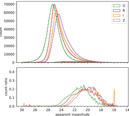
The Australian Dark Energy Survey (OzDES;Yuan et al. 2015) is a targeted spectroscopic follow-up of DES which uses the AAOmega spectrograph (Smith et al. 2004) on the 3.9 meter Anglo-Australian Telescope (AAT). Coupled with the Two Degree Field (2dF) 400-ﬁbre multi-ﬁbre positioning system (Lewis et al. 2002). Data Release 1 provides spectroscopy for 280 000 sources of which 244 000 have reliable spectroscopic redshifts (Childress et al. 2017). The top panel of Figure 1.1 shows histograms of source counts for each of the four DES photometric bands: reliably reaching magnitudes as faint asmR ă25. The bottom panel of Figure 1.1 shows the per-bin ratio of DES sources with an OzDES redshift for each photometric band. The spec-troscopic completeness is established and used in§3. Throughout this thesis DES multi-band catalogueI-band astrometry is used for optical source positions, and source visualisation.

0 10000 20000 30000 40000 50000 60000 70000

count

G R I Z

14 16 18 20 22 24 26 28 30

apparent magnitude 0.0

0.1 0.2 0.3 0.4

[image:27.595.175.421.421.643.2]

count ratio

Figure 1.1:Source counts per photometric band (G,R,I,Z) for DES op cal photometry. The bo om pane shows the

(28)

1.3 Infrared Data: SWIRE

Spitzer Wide-Area InfraRed Extragalactic Survey (SWIRE;Lonsdale et al. 2003) has detected 2 million IR-selected galaxies sources over„49 deg2in six ﬁelds. The infrared photometry used in this thesis are MIPS 3.6 – 24μm channels. At 3.6μm SWIRE achieves 5σsensitivities of 5μJy and a full-width at half-maximum (FWHM) resolution of 1.22_{, and at 24}_{μm 5}_σ_{sensitivities of}

200μJy at spatial resolution of 5.52_{(Surace et al. 2005). SWIRE source positions used herein}

are drawn from 3.6μm IRAC data which is complete to„ 97 per cent at 400μJy (Babbedge et al. 2006).

1.4 Cross-Matching Multi-Frequency Catalogues

Difficulties arise in the correct handling of multiple source catalogues when these catalogues originate from different instrumentation; especially when cross-matching optical or infrared source positions with radio source positions. Compared to the accurate astrometry and rela-tively high resolution of optical surveys, radio surveys use peak-ﬁnding algorithms to estimate positions of often diffuse or extended radio sources (e.g.,Franzen et al. 2015). For isolated, com-pact radio galaxies this technique is sufficiently accurate; however, in dense ﬁelds, the radio sources are non-Gaussian and determining the centre of the radio emission becomes guess-work.

An uncertainty in radio source location is especially concerning when cross-matching in a dense optical or infrared field. It then becomes difficult to identify which source of many poten-tial matches is the counterpart of a particular radio peak (e.g., Figure 1.2c). If the observational ‘depth’ of the radio and optical (or infrared) surveys are not well matched, then all issues with correct multi-frequency source association are exacerbated. Potential dense-field misassocia-tion can be somewhat corrected if cross-matching is conducted manually by an expert, as she or he can comment and flag such sources for more careful statistical consideration. If however, automated positional cross-matching is used then poorly matched resolution and survey depth becomes a source forsystematicerror, preferentially misidentifying dense cluster sources.

1.4.1 Matches and Mismatches

Software such as TOPCAT:_{can very efficiently perform a sky-coordinate positional}

cross-matching between two catalogues. However, this easy-to-use software has no discretion for physical distribution or orientation of sources, nor can it provide confidence of match; for ex-ample in the event of a dense pairing field. This means we have to accept each match as correct whilst understanding that a large percentage of total matches will be incorrect. An incorrect match would constitute a match to a foreground or background galaxy in the optical (or in-frared) catalogue unrelated to the radio source. Such a mismatch could arise from: a poorly located radio-flux peak (Figure 1.2aand Figure 1.4); a non-detection of an optical or infrared

(29)

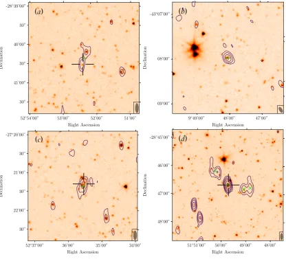
counterpart (Figure 1.2b); a single radio component encompassing a cluster of optical or in-frared sources (Figure 1.2c); or isolated radio lobes of an extended AGN positionally matched to a coincident background galaxy (Figure 1.2d). For the remainder of this chapter, I will broadly refer to these incorrect matches as contaminants, spurious matches, or false matches.

In the case of sources where a host galaxy is misidentiﬁed, it begins to introduce a luminosity bias to our results. Due to instrumentation limits, a mismatch will favour a brighter (appar-ent magnitude) optical counterpart than the correct host. Because radio sources tend to be higher redshift than optical sources, a mismatched optical source is likely to be from a closer redshift causing the radio luminosity calculated from that redshift to be underestimated. If a given source belongs at a higher redshift but is mismatched to a lower redshift, then the lu-minosity calculated from the ﬂux of this source is lower than the physical lulu-minosity, and the source has been shifted away from its high-redshift population. Practically this has created an under-counting of bright, distant sources and an over-counting of nearby faint sources. Accu-mulating many of these errors over a large catalogue would result in a systematic luminosity error. With the possibility of vast differences in correct and chosen redshifts, and such mistakes being frequent, the result would be the fabrication of many faint radio sources.

Another issue with the automatic cross-matching method arises from the extended radio sources that make up a small fraction of the AGN in our sample. In blind nearest neighbour (BNN) cross-matching isolated lobes are almost always associated with a coincident, unrelated, optical source (e.g.,Figure 1.2d). Without manual intervention or a sophisticated automatic al-gorithm (e.g.,Fan et al. 2015) this is guaranteed because nearest-neighbour matching has no in-formation to understand that these lobes are not genuine galaxies#_{. Further to the luminosity} error mentioned above, this introduces an over-counting of true radio sources, and an underesti-mation of the combined ﬂux of the correct radio host;_{. Whilst there are relatively few of these}

sources in the ATLAS catalogue, these sources dominate the high-luminosity end of the radio luminosity function; as such, correctly calculating their luminosity and distance is essential for the correct accounting of the spatial densities of galaxies, especially at high redshift where the detection rate of faint sources has diminished.

1.5 Comparison of Cross-matching Techniques

The ﬁnal two chapters of this thesis rely upon the availability of accurate redshifts and spectra for as many of our ATLAS sources as possible. Methodology aside, associating an ATLAS radio

#_{There is an emerging research ﬁeld that hopes to identify isolated lobes automatically, but it either}

relies upon AGN hot-spots of similar ﬂux symmetrically centered about a radio core, or using Bayesian statistical weighting that encroaches upon supervised machine learning (e.g.,Fan et al. 2015). Neither of these methods would be considered ablindnearest-neighbour cross-matching technique.

;_{I the case of a typical double lobed AGN with a faint core and bright hot-spots this error would}

(30)

52◦_54’00” _53’00” _52’00” _51’00”

-28◦_39’00”

30”

40’00”

30”

41’00”

30”

Right Ascension

Declination

(a)

9◦_49’00” _48’00” _47’00”

-43◦_07’00”

08’00”

09’00”

Right Ascension

Declination

(b)

52◦_37’00” _36’00” _35’00” _34’00”

-27◦_20’00”

30”

21’00”

30”

22’00”

30”

Right Ascension

Declination

(c)

51◦_51’00” _50’00” _49’00” _48’00”

-28◦_45’00”

46’00”

47’00”

48’00”

Right Ascension

Declination

[image:30.595.92.509.128.505.2]

(d)

Figure 1.2:Four examples of scenarios that would result in an incorrect cross-match if the cross-matching were done by an

automa c method without topographical informa on: ﬁgures were generated from MCVCM. In each panel1.4GHz, ATLAS radio con nuum contours are overlaid onto SWIRE3.6μm infrared emission, contour levels are2n_{ˆ x}_RMS_y_{calculated for}

each cutout. The large black cross-hair shows the loca on of the user-selected infrared core, and the green crosses show the loca on of the selected radio component peaks. In the bo om right of each image is the ATCA beam for that ﬁeld. Panela

(31)

52◦06’00” 05’00” 04’00” 03’00” -27◦40’30”

41’00” 30” 42’00” 30” 43’00” Right Ascension Declination

52◦06’00” 05’00” 04’00” 03’00” -27◦40’00”

30” 41’00” 30” 42’00” 30” Right Ascension Declination

52◦06’00” 05’00” 04’00” 03’00” -27◦40’30”

53◦08’00” 07’00” 06’00” -27◦43’00”

30” 44’00” 30” 45’00” Right Ascension Declination

53◦09’00” 08’00” 07’00” 06’00” -27◦43’00”

53◦45’00” 44’00” 43’00” -27◦47’00”

30” 48’00” 30” 49’00” Right Ascension Declination

53◦45’00” 44’00” 43’00” -27◦46’00”

[image:31.595.91.493.161.542.2]

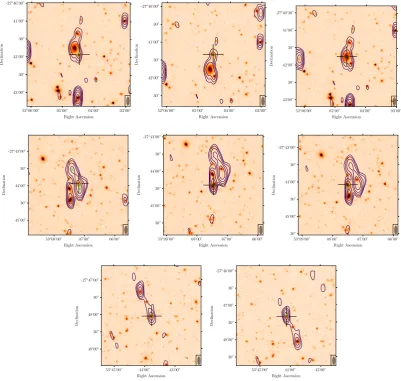
Figure 1.3:Three MCVCM examples of scenarios where the automa c source-ﬁnding algorithm (Franzen et al. 2015)

(32)

52◦02’00” 01’00” 00’00” -27◦50’00”

52◦04’00” 03’00” 02’00” -27◦54’30”

52◦10’00” 09’00” 08’00” 07’00” -27◦46’30”

52◦15’00” 14’00” 13’00” -27◦59’00”

30”

-28◦00’00”

30”

01’00”

30”

Right Ascension

Declination

52◦26’00” 25’00” 24’00” -28◦01’30”

52◦38’00” 37’00” 36’00” -28◦40’30”

52◦32’00” 31’00” 30’00” -28◦29’30”

52◦21’00” 20’00” 19’00” -28◦09’30”

52◦43’00” 42’00” 41’00” -28◦07’30”

[image:32.595.90.498.176.552.2]

08’00” 30” 09’00” 30” Right Ascension Declination

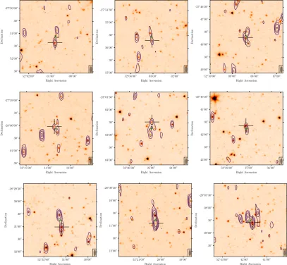
Figure 1.4:Nine MCVCM examples of scenarios where the automa c source-ﬁnding algorithm (Franzen et al. 2015) merged

(33)

source with an OzDES targeted spectrum can take two pathsκ(hereafter referred to as data-paths):

• ATLAS 1.4 GHz radio matched directly to DES optical photometry

• ATLAS 1.4 GHz radio matched to DES optical photometry via the SWIRE 3.6μm in-frared catalogue as an intermediate step

The possible beneﬁt of an infrared intermediary comes from the relationship between the infrared and 1.4 GHz radio emission discussed in§0.3, along with the empirical evidence that

ą 90 per cent of optical galaxies are radio-quiet (Norris et al. 2006). For an optical survey limited to the same redshift range as a radio or infrared survey, there will be a higher density of detections in the optical survey. In practice, this causes an over-crowding effect when try-ing to match radio and optical catalogues that is often combated by performtry-ing a magnitude cut of the optical catalogue before matching to the radio catalogue (e.g.,Sadler et al. 2007; Donoso et al. 2009;Pracy et al. 2016). This cut is made on the basis of an assumption that, at its core, assumes ‘bright things are bright’; that is, fainter optical sources are not likely hosts to a bright radio galaxy. I will show later in this section that there are sufficiently many ‘correct’ faint optical counterparts to make such a technique undesirable for an unbiased ﬁnal cata-logue. In this chapter, I aim to conﬁrm that the cumulative position uncertainty between the radio, infrared, and optical catalogues will be smaller than the direct uncertainty between ra-dio and optical catalogues. I also aim to generate a reliable multi-frequency catalogue by vi-sually cross-matching sources and to compare this to a catalogue cross-matched using simple nearest-neighbour cross-matching.

There are several techniques used for cross-matching of catalogue pairs, some that will be covered or discussed in this thesis are:

• blind nearest-neighbour (BNN) positional matchingϱ_,

• manual matching of sources via visual catalogue inspection,

• custom machine learning, or Bayesian algorithms (e.g.,Fan et al. 2015;Lukic et al. 2018),

• citizen scientist visual matching (e.g.,Banﬁeld et al. 2015).

The third and fourth techniques will be brieﬂy discussed later in this chapter, but they are considered ‘intelligent’ automation and are beyond the scope of this work; these techniques re-quire a pre-existing‘golden standard’cross-matched catalogue for training and comparison. This chapter aims to establish such a standard by conducting and evaluating the ﬁrst two techniques (BNN and visual matching) for both of our data-paths.

κ_{in all analyses I have performed a nearest-neighbour cross-matching of DES photometry to OzDES} targeted spectroscopy, and assume that this cross-matching is sufficiently accurate not to affect our ﬁnal ATLAS redshifts regardless of cross-matching technique or data-path.

ϱ_{blind, in this sense, refers to the matching algorithm having no topographical or physical}

(34)

1.6 Blind Nearest-Neighbour Cross-Matching

The cross-matching of two catalogues using a BNN technique only requires the speciﬁcation of a matching radius. A radius that is too small compromises the completeness of the ﬁnal catalogue, whilst with a sufficiently large matching radius, the catalogues can be matched to 100 per cent completion, but it becomes increasingly likely that those matches are spurious. In the following sections, I will discuss the reliability of cross-matching via BNN and establish an automated, repeatable method for choosing a cross-matching radius that maximises reliability.

1.6.1 Evaluating Blind Nearest-Neighbour Cross-Matching

To establish a standardised method for calculating a ‘best-ﬁt’ cross-matching radius, I assess the increase in cross-match counts as cross-matching radius is increased. To quantify com-pletion, this is performed for the cross-matching of our primary and secondaryגcatalogues, whereas the number of false matches is quantiﬁed by cross-matching the primary catalogue to a randomised pairing catalogue. The random catalogue is generated by perturbing the right-ascension and declination of each source from the secondary catalogue by a random amount. This random perturbation (δ_r) is drawn from a range spanning´452 _ă _δ

r ă 452(see Ap-pendix§B for a full justiﬁcation). The completeness,C, of each catalogue pairing is deﬁned as the fraction of total ATLAS catlogue sources with a match, regardless of validity.Cis calcu-lated as a function of radius as:

Cprq “ Nprq

NATLAS

(1.1)

For these catalogue pairings, a fraction of the total matches will be incorrect spurious matches or contaminants. It is effectively impossible to discover which of our matches between the pri-mary and secondary catalogues are false, but the percentage of false matches can be estimated by performing the cross-matching between our primary catalogue and a randomised secondary catalogue.

The number of false matches will also increase as the cross-matching radius is increased, and the spurious fraction,S, is deﬁned as:

Sprq “ Nrandprq

NATLAS

. (1.2)

The variableNrandis the number of matches between the primary catalogue (ATLAS in this

example) and the random catalogue described above. In both of these equations,NATLASis the

total number of sources in the ATLAS catalogueℵ.

ג_{In all cases the secondary catalogue is the catalogue with the greatest source density.}

(35)

In this chapter, I cross-match ATLAS 1.4 GHz with the SWIRE 3.6μm infrared catalogue, and ATLAS 1.4 GHz with DES photometric catalogue. I also cross-match DES with OzDES, and SWIRE with DES so that I can build a ﬁnal ATLAS–DES–SWIRE–OzDES catalogue for both data-paths.

1.6.2 Blind Nearest-Neighbour Cross-Matching: OzDES–DES

Because OzDES data are from targeted follow-up of DES photometric sources we expect to see reliable BNN cross-match pairing of these two catalogues. This result is conﬁrmed by Figure 1.5: a visualisation of the number of matches obtained per matching radius bin for a blind nearest-neighbour search. For these data, we can obtain practically 100 per cent completeness with only 4 per cent contamination, the matching radius required to achieve this is just 0.862_{. As}

an aside, there is an interesting double-Gaussian feature (peaks: 0.052_{, 1.20}2_{) for the}

cross-matching of these catalogues. This arises from the different instrumentation used to obtain the DES photometry in the CDFS and ELAIS-S1 ﬁelds compared to those instruments used for other DES regions (Childress et al. 2017).

1.6.3 Blind Nearest-Neighbour Cross-Matching: SWIRE–DES

Since I will also be cross-matching to DES photometry via the SWIRE infrared catalogue, I need to establish a similar cross-matching basis for the DES–SWIRE pairings. Figure 1.5 shows similar reliability as with DES–OzDES cross-matching:„100 per cent completeness with only 6 per cent contamination at a radius of 1.152_{; this radius is similar to cross-matching radii used}

for pairing SWIRE infrared and other optical catalogues (Surace et al. 2005;Rowan-Robinson et al. 2008). These cross-matching results are sufficiently reliable that I assume an exact match of each ATLAS source to an OzDES redshift, where the appropriate matches are present in the subsequent catalogues.

1.6.4 Blind Nearest-Neighbour Cross-Matching: ATLAS–SWIRE & ATLAS–DES

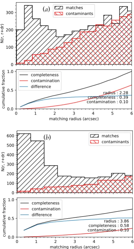
Now that I have established a reliable DES–OzDES, and SWIRE–OzDES redshift association to use with both of the data-paths, I can investigate the difference between BNN cross-matching and manual visual cross-matching of ATLAS. Because the precision of ATLAS source positions is much lower than either DES or SWIRE due to lower resolution and ATLAS source blend-ing, I expect poor performance from a BNN technique. This is apparent upon inspection of Figure 1.6 which visualises BNN cross-matching in the same manner as Figure 1.5. This time instead of choosing an optimum cross-matching radius based on a radius at which we reach„

(36)

0 1000 2000 3000 4000

N(r, r+dr)

matches contaminants

0.0 0.2 0.4 0.6 0.8 1.0

matching radius (arcsec) 0.0

0.5 1.0

cumulative fraction

radius : 0.86 completeness : 0.99 contamination : 0.04 completeness

contamination difference

(a)

0 1000 2000 3000 4000 5000

N(r, r+dr)

0.0 0.2 0.4 0.6 0.8 1.0

0.5 1.0

cumulative fraction

[image:36.595.185.409.138.551.2]

(b)

Figure 1.5:Top: OzDES–DES; Bo om: SWIRE–DES. Visualisa on of the eﬀect of increasing cross-matching radius for blind

(37)

Table 1.1:Comparison of the op mum radii for cross-matching our catalogues. The ﬁrst column indicates the catalogues being cross-matched in the format ‘primary–secondary’. The ‘Completeness Frac on’ column is the total frac on of sources with a cross-match (Equa on (1.1)). The ‘Spurious Frac on’ column is the frac on of matches between the primary catalogue and a randomly disassociated pairing catalogue generated from the secondary catalogue (Equa on (1.2)).

Radius (arc seconds) Completeness Frac on Spurious Frac on

DES – OzDES 0.86 0.99 0.04

SWIRE – DES 1.15 0.99 0.06

ATLAS – DES 2.28 0.39 0.10

ATLAS – SWIRE 3.86 0.58 0.10

completeness. Attempting to increase completeness by increasing the matching radius would only serve to decrease the ﬁnal catalogue reliability by increasing the spurious fraction. Ta-ble 1.1 summarises the optimum BNN cross-matching radii decided by this technique.

It is clear from these results that BNN cross-matching via either of these data-paths would result in a catalogue with both poor completeness and a high number of spurious matches. It is promising to see, however, that there is a definite improvement in catalogue completeness versus contamination when matching ATLAS to SWIRE compared with matching ATLAS to DES. Importantly, I have established that the reliability of cross-matching DES to OzDES and SWIRE to OzDES are nearly identical, so the improvement of using the SWIRE catalogue as an intermediate cross-matching step carries through to our final redshift acquisition. In the con-struction of the final BNN catalogue, I use the cross-matching radii established in this section.

1.7 Multi-Catalogue Visual Cross-Matching (MCVCM)

Visually inspecting each of our 5118 ATLAS radio sources and manually associating an infrared or optical counterpart is arduous and requires precise book-keeping. There is sufficient room for user error to justify the development of a semi-automated program to manage the back-end, freeing the expert to focus on the correct classiﬁcation of sources. For the sake of expediency and repeatability, it is essential to have as much of this automated as possible. Developing a tool to achieve this task that is generalised enough to be usable for the broader astronomy com-munity has been a large part of this thesis. Whilst there have been small software programs written by others to handle facets of this task, they mostly involved the generation of visual cutouts with the intention of manual book-keeping by the user; or the expert is restricted to a yes or no conﬁrmation of a BNN match (e.g.,Norris et al. 2006,2007). Radio Galaxy Zoo (RGZ) and LOFAR galaxy zoo (Williams et al. 2018) use closed-source professionally developed software to perform this task for their sample. This interface is designed to allow their citizen scientists to make selections without worrying about the data handling. Since RGZ is unavail-able for distribution, I have written MCVCM as an open-source Python program to emulate the RGZ interface.

(38)

0 100 200 300

N(r, r+dr)

0 1 2 3 4 5 6

0.5 1.0

cumulative fraction

(a)

0 100 200 300 400 500 600

N(r, r+dr)

0 1 2 3 4 5 6

0.5 1.0

cumulative fraction

[image:38.595.184.410.141.559.2]

(b)

Figure 1.6:Top: ATLAS–DES; Bo om: ATLAS–SWIRE. Visualisa on of the eﬀect of increasing cross-matching radius for

(39)

source. Provided that the images and catalogues are in standard ‘.ﬁts’‹_{format, the end user}

need only provide for each ﬁeld:

• radio continuum image ﬁle,

• radio RMS image ﬁle,

• optical/infrared image ﬁle,

• radio positions catalogue (primary),

• optical/Infrared positions catalogue (secondary).

Once configured to read these files, MCVCM will produce an image cutout centred on the first source in the primary catalogue˛_{; this cutout will appear as radio contours overlaid onto}

an optical or infrared image≀. Across three phases, the user will select an infrared galaxy core (if there is an appropriate candidate) followed by any radio peaks associated with that core. The user performs this selection by clicking marks representing the right ascension and decli-nation of the catalogue sources (see Figure A.1dPage 80). During cross-matching, the user can increase the field of view of the cutout to better gauge the environment. Optionally, they may also enter an integer confidence flag at any point (P t1,2,3,4u), as well as a comment string for later reference. Once the user is satisfied and moves to the next source, MCVCM will ap-pend to a new catalogue file all information from the primary catalogue for the selected radio sources, the user flag and user comment, as well as a unique association string used to link all radio components to the infrared host selected from the secondary catalogue. The MCVCM software includes a suite of functionality to facilitate better cross-matching and to ensure no loss of progress in the event of a software or computer crash. See Appendix§A for a thorough breakdown of MCVCM, including instructions, examples, the web address of the online reposi-tory from which it can be accessed.

1.7.1 Considerations of Visual Cross-Matching

Selecting the correct infrared or optical counter-part for our ATLAS sources is vital for devel-oping a rigorous cross-matched catalogue that can be used as a golden standard for training intelligent automated cross-matching systems. Suppose a radio component is erroneously as-sociated with a brighter, low-redshift infrared or optical counterpart. In this case, the radio luminosity is underestimated (as the measured ﬂux is now attributed to a closer source) and the number of nearby low-luminosity sources is artiﬁcially increased. Additionally, a bright radio

‹_{Flexible Image Transport System (}_{Calabretta & Greisen 2002}_).

˛_{The primary catalogue is generally the catalogue with the fewest sources. In the case of this thesis}

that is the ATLAS 1.4 GHz component catalogue. This is not a strict requirement of MCVCM, but it does reduce the number of iterations for the user.

(40)

source is removed from a higher redshift bin. If instead, the user is to manually ignore such a source (that is, treat it as a non-detection) then the reliability of our catalogue increases. When I construct radio luminosity functions in§3 volume corrections of the population statistics will be used to correct for these non-detections, making this the preferred option.

I found that during the visual cross-matching there is a temptation to try to match as many sources as possible, perhaps in an unconscious attempt to maximise matching completeness. However, it is essential when making these cross-match selections to not ‘select the closest’ source; careful consideration must be made for the topography. Occasionally there will be a radio source with an aligned infrared source that is visible in MCVCM, but has fallen below the detection limit of the SWIRE survey (e.g., Figure 1.2a). It is very likely that this undetected faint source is indeed the true host, and if one is to select a nearby source that is merely ‘close enough’, then we run into a problem of ‘false’ cross-identiﬁcation (see§1.4), it is instead better practice to leave this as an unmatched source.

Because the DES optical survey contains a higher density of sources than 3.6μm SWIRE infrared survey (80 000 deg´2_{versus 31 000 deg}´2_{) there are many more ‘chance alignments’ for}

a given ATLAS source when visually cross-matching to DES; therefore, the chance of making a false cross-identiﬁcation is increased: even if one is careful to avoid them. As discussed in §1.5, it is common practice when conducting BNN cross-matching to make a magnitude cut for the optical catalogue to reduce the number of potential candidates for a spurious match. However, one of the beneﬁts of manually cross-matching is that it alleviates the need to impose potentially biasing magnitude assumptions upon the data. For this reason, I have retained all sources from each catalogue and made cross-matching selections purely based on the visual information.

I also expect that this excess of sources will increase the variability of ﬁnal cross-matched catalogues if a single user or many users perform several cross-matching runs.Banﬁeld et al. (2015) developed a ‘consensus algorithm’ that weighted contributions from a large user-base, unfortunately with only one complete visual cross-matching pass for both ATLAS–SWIRE, and ATLAS–DESqI am unable to quantify variability errors.

1.7.2 Difficulties With Visual Cross-Matching of ATLAS–DES

Manually cross-matching ATLAS against DES requires that the collection of 11_ˆ₁1_DES

opti-cal image tiles are mosaicked together/. Without mosaicking it would be very difficult to verify larger multi-component structures as they invariably exist across several tiles (e.g., Figure 1.7). Comparatively, once SWIRE image tiles are mosaicked they are full-ﬁeld with no gaps. Once

q_{Through the course of developing MCVCM I did perform many partial passes, but these were} not included in the ﬁnal analysis as I wanted to be certain that I was cross-matching with a consistent technique and error tolerance.

/_{Mosaicing is performed using montage (}_{Jacob et al. 2010}_;_{Berriman et al. 2016}_,

(41)

the data is in the appropriate format I followed the procedure outlined in§1.7 for the 5118 AT-LAS radio components.

During MCVCM cross-matching of ATLAS–DES there were many cases when the density of the DES catalogue source detections made the selection of a likely optical galaxy difficult, in these cases, I deferred the selection to the brightest of the candidates. There is also a substantial difference in ﬁeld overlap of SWIRE and DES with the ATLAS survey (see Figure 1.8). Many of the visual ATLAS–DES cross-matches had to be skipped as there were no available DES images or sources in these regions, this would compromise the performance of the ATLAS–DES cross-matching, compared to ATLAS–SWIRE for which the overlap is more complete.

Figure 1.7:Op cal MCVCM cutout of ATLAS source CI0304.1.4GHz ATLAS radio con nuum contours are overlaid onto

DES (11 _ˆ₁1_{) mosaicked}_I_´_{band les. Radio contour levels are}₂n_{ˆ x}_RMS_y_{calculated for this ﬁeld of view (see}

Fig-ure 1.2(d) Page 15 for the3.6μm infrared cutout of this source).

1.7.3 Comparing Cross-Matching Techniques

(42)

CDFS

ELAIS-S1

Figure 1.8:Overlap of ATLAS, DES, and SWIRE for ELAIS-S1 and CDFS. The red line marks the bounding edge of SWIRE, the

(43)

From the initial 5118 detections in the ATLAS catalogue MCVCM cross-matching (via DES and SWIRE) veriﬁes 4903 individual galaxies of which 137 are extended or multi-component sources. Visual cross-matching against the SWIRE infrared catalogue results in an infrared counter-part for 95 per cent (4658) sources. In Table 1.2 I have treated these 4658 sources as correct for comparison of techniques and data-pathsı. Table 1.2 compares how many of the matches from each of the other methods would result in an identical ATLAS–SWIRE–DES– OzDES pairing.

Table 1.2:Comparison of the quality of the four combina ons of cross-matching techniques and data-paths: as indicated

by the ﬁrst two columns. The results from the visual cross-matching of ATLAS to SWIRE (shown in the ﬁrst row) is used as our standard of comparison. TheTotalcolumn is the number of ATLAS sources with a match via the associated method. The

‘Correct’column is the total number of sources that have the same ﬁnal infrared counterpart as ‘visual - SWIRE’. TheCorrect Frac oncolumn is this ra o of‘Correct’matches and theTotalmatches. TheCompletenesscolumn is the ra o of‘Correct’to the total ATLAS source count (4903). Note that for the two BNN techniques I have already restricted the cross-matching radius to limit spurious matches to 10 per cent (see Figure 1.6) this will increase the reliability of the ﬁnal catalogue at the expense of completeness.

Data-path Technique Total ‘Correct’ Correct Frac on Completeness

ATLAS–SWIRE Visual 4658 4658 - 0.95

ATLAS–SWIRE BNN 2185 2135 0.98 0.44

ATLAS–DES Visual 3905 2776 0.71 0.57

ATLAS–DES BNN 1972 1870 0.95 0.38

The ﬁrst point to note is that regardless of the technique used, cross-matching via the 3.6μm SWIRE infrared catalogue yields a greater number of total matches, and a better‘Correct Frac-tion’, in the case of BNN.

Another notable point is that regardless of the data-path, visual cross-matching results in many more total matches. Of course, increasing the matching radius for BNN would increase the total number of matches for this technique, but as established in§1.6 this would only serve to compromise the ﬁnal sample with spurious matches. Ideally, visual cross-matching would result in 100 per cent reliability, but that is not the case.

Inspecting the correct fraction of visual matches for the ATLAS–DES cross-matching, almost 30 per cent of the matches resulted in an incorrect ﬁnal SWIRE infrared core ℘. In§1.5 I ar-gued that having„ 300 per cent more sources per square degree in the DES survey compared to the SWIRE survey would result in many more spurious matches. Figure 1.9 is a visual demon-stration of these effects; because the OzDES survey contains a much higher source density, and the data is high-resolution (compared to ATLAS) the BNN algorithm can ﬁnd a match for each ATLAS source within a small search radius, regardless of validity. The MCVCM cross-matching (i.e., VIS SWIRE, and VIS OzDES) illustrates the ‘true distribution’ of source separations for

ı_{I by no means assume that visual matching is 100 per cent reliable, I assume that it is more reliable}

than BNN and merely use the results as a basis for comparison

(44)

0 1 2 3 4 5 6 source separation (arcsec)

0 50 100 150 200 250

N

VIS SWIRE VIS DES BNN SWIRE BNN DES

Figure 1.9:Comparison of separa on between ATLAS 1.4 GHz source posi on and the respec ve SWIRE or OzDES

posi-ons for each data-path: visual cross-matching (MCVCM), or blind nearest-neighbour (BNN).

these data due to the nature of visual cross-matching (that is, the low-resolution of ATLAS 1.4 GHz data is accounted for during visual inspection). Comparing the source separations for SWIRE BNN to these ‘true distributions’ shows closer agreement than OzDES BNN, suggesting that better matched survey source density and resolution allows for the a better chance of a ﬁnal BNN matched catalogue with few spurious matches.

It is worth noting that the order in which I did the MCVCM cross-matching may have af-fected the visual cross-matching results: I cross-matched ATLAS–DES, and later cross-matched ATLAS–SWIRE. It is likely that I acquired visual biases during the ﬁrst cross-matching that I inadvertently applied to the second cross-matching. This may have marginally ampliﬁed the ratio of erroneous matches between data-paths, but would require several iterations of cross-matching by independent experts to quantify these biases.

1.8 Final ATLAS radio catalogue

(45)

catalogue compared to directly cross-matching to DES optical catalogue.

1.8.1 Photometric and Spectroscopic Counterparts

For each of the DES photometric bands, Figure 1.10 shows the breakdown of matches to the ATLAS radio catalogue separated into the cross-matching techniques and data-paths: visual SWIRE–ATLAS; visual DES–ATLAS; BNN SWIRE–ATLAS; BNN DES–ATLAS. In all cases, visual ATLAS–SWIRE cross-matching performs the best which is likely due to the similar galac-tic emission processes producing radio and infrared emission that have been discussed above, as well as the lower surface density of SWIRE sources compared to DES sources decreasing the frequency of spurious matches.

1.8.2 Conclusion

The next generation of radio sky surveys will yield on the order of millions of sources as modern instrumentation improves data quality and quantity (Norris 2017). For the several thousand sources available in the ATLAS DR3 survey, cross-matching multi-frequency catalogues via manual source inspection is both practical and beneﬁcial for the integrity of the data. For sam-ples consisting of a few tens of thousands of sources, the resource commitment to such a task becomes questionable, and for catalogues with millions of sources, it becomes futile. To accom-modate the next generation of large data various techniques are being developed to automate or delegate such time-intensive tasks. These techniques which include citizen science (Banﬁeld et al. 2015) and machine learning (Lukic et al. 2018) require training data or comparison data to verify their legitimacy. Having now developed a sample of several thousand reliably cross-matched sources, we have a better groundwork on which to build this software.

(46)

0 100 200 300 400 500 600 Total Count

VIS SWIRE (3269) VIS DES (2719) BNN SWIRE (2109) BNN DES (1847)

10.0 12.5 15.0 17.5 20.0 22.5 25.0 27.5 30.0

apparent magnitude (G) 400

200 0

Count Difference

10.0 12.5 15.0 17.5 20.0 22.5 25.0 27.5 30.0

apparent magnitude (R)

0 100 200 300 400 Total Count

10.0 12.5 15.0 17.5 20.0 22.5 25.0 27.5 30.0

apparent magnitude (I) 400

200 0

Count Difference

10.0 12.5 15.0 17.5 20.0 22.5 25.0 27.5 30.0

apparent magnitude (Z)

Figure 1.10:Per-bin DES photometry source counts for the cross-matching methods discussed for each of the four DES

(47)

If people sat outside and looked at the stars each night, I’ll bet they’d live a lot differently.

– Calvin (& Hobbes)

2

Diagnostic Population Segregation of

ATLAS Radio-Galaxies

2.1 Discerning Galaxy Characteristics

Absolute segregation of galaxies into sub-populations is inherently an unachievable goal. Galax-ies do not occupy discrete population spaces for which there exists an obscure combination of observables that will allow us to unlock their real identities. Not only are galaxies the most complex systems in the Universe but they are the systems for which we have the least (and most contaminated) information. Electromagnetic radiation, from its various origins, is the only source of information for understanding these incomprehensibly vast celestial bodies. This light originates from a multitude of mechanisms and travels to our single point of reference over the course of aeons over which time and space it can have countless interactions obfuscating or obliterating the original information.