This is a repository copy of Chromatic index of graphs with no cycle with a unique chord
.
White Rose Research Online URL for this paper:
http://eprints.whiterose.ac.uk/74348/
Article:
Machado, RCS, de Figueiredo, CMH and Vuskovic, K (2010) Chromatic index of graphs
with no cycle with a unique chord. Theoretical Computer Science, 411 (7-9). 1221 - 1234 .
ISSN 0304-3975
https://doi.org/10.1016/j.tcs.2009.12.018
Reuse
See Attached
Takedown
If you consider content in White Rose Research Online to be in breach of UK law, please notify us by
Chromatic index of graphs with no cycle with a unique chord
R. C. S. Machado∗,†, C. M. H. de Figueiredo∗, K. Vuˇskovi´c‡
February 8, 2009
Abstract
The class C of graphs that do not contain a cycle with a unique chord was recently studied by Trotignon and Vuˇskovi´c [26], who proved strong structure results for these graphs. In the present paper we in-vestigate how these structure results can be applied to solve the edge-colouring problem in the class. We give computational complexity results for the edge-colouring problem restricted toC and to the sub-class C′ composed of the graphs ofC that do not have a 4-hole. We
show that it is NP-complete to determine whether the chromatic index of a graph is equal to its maximum degree when the input is restricted to regular graphs ofC with fixed degree ∆ ≥3. For the subclass C′,
we establish a dichotomy: if the maximum degree is ∆ = 3, the edge-colouring problem is NP-complete, whereas, if ∆6= 3, the only graphs for which the chromatic index exceeds the maximum degree are the odd order cycle-graphs and the odd order complete graphs, a charac-terization that solves edge-colouring problem in polynomial time. We determine two subclasses of graphs in C′ of maximum degree 3 for
which edge-colouring is polynomial. Finally, we remark that a conse-quence of one of our proofs is that edge-colouring in NP-complete for
r-regular tripartite graphs of degree ∆≥3, forr≥3.
Keywords: cycle with a unique chord, decomposition, recognition, Petersen graph, Heawood graph, edge-colouring.
1
Motivation
LetG= (V, E) be a simple graph. The degree of a vertex v inGis denoted degG(v), and the maximum degree of a vertex in G is denoted ∆(G). An
∗COPPE, Universidade Federal do Rio de Janeiro, Rio de Janeiro, RJ, Brazil. E-mail:
{raphael,celina}@cos.ufrj.br.
†Instituto Nacional de Metrologia Normaliza¸c˜ao e Qualidade Industrial
‡School of Computing, University of Leeds, Leeds LS2 9JT, United Kingdom. Email:
edge-colouring of G is a function π : E → C such that no two adjacent edges receive the same colourc∈C. If C={1,2, ..., k}, we say thatπ is a k-edge-colouring. Thechromatic index of G, denoted by χ′(G), is the least kfor which Ghas a k-edge-colouring.
Vizing’s theorem [27] states thatχ′(G) = ∆(G) or ∆(G)+1, defining the classification problem: graphs with χ′(G) = ∆(G) are said to be Class 1, while graphs with χ′(G) = ∆(G) + 1 are said to be Class 2. The edge-colouring problem orchromatic index problem is the problem of determining the chromatic index of a graph. Edge-colouring is a challenging topic in graph theory and the complexity of the problem is unknown for several important well studied classes. Edge-colouring is NP-complete for regular graphs [13, 18] of degree ∆≥ 3. The problem is NP-complete also for the following classes [5]:
• r-regular comparability (hence perfect) graphs, forr ≥3;
• r-regular line graphs of bipartite graphs (hence line graphs and clique graphs), for r≥3;
• r-regulark-hole-free graphs, forr ≥3,k≥3; • cubic graphs of girthk, fork≥4.
Graph classes for which edge-colouring is polynomially solvable include the following:
• bipartite graphs [14];
• split-indifference graphs [21];
• series-parallel graphs (hence outerplanar) [14]; • k-outerplanar graphs [2], fork≥1.
The complexity of edge-colouring is unknown for several well-studied strong structured graph classes, for which only partial results have been reported, such as cographs [1], join graphs [10, 11, 19], cobipartite graphs [19], planar graphs [24, 28], chordal graphs, and several subclasses of chordal graphs such as indifference graphs [8], split graphs [7] and interval graphs [3].
Trotignon and Vuˇskovi´c [26] studied the class C of graphs that do not contain a cycle with a unique chord. The main motivation to investigate this class was to find a structure theorem for it, a kind of result which is not very frequent in the literature. Basically, this structure result states that every graph inC can be built starting from a restricted set of basic graphs and ap-plying a series of known “gluing” operations. Another interesting property of this class is that it belongs to the family of theχ-bounded graphs, intro-duced by Gy´arf´as [12] as a natural extension of perfect graphs. A family of graphs G is χ-bounded withχ-binding function f if, for every induced sub-graph G′ of G ∈ G, χ(G′) ≤f(ω(G′)), where χ(G′) denotes the chromatic number of G′ and ω(G′) denotes the size of a maximum clique in G′. The research in this area is mainly devoted to understanding for what choices of forbidden induced subgraphs, the resulting family of graphs is χ-bounded, see [23] for a survey. Note that perfect graphs are a χ-bounded family of graphs withχ-binding functionf(x) =x, and perfect graphs are character-ized by excluding odd holes and their complements. Also, by Vizing’s The-orem, the class of line graphs of simple graphs is aχ-bounded family with χ-binding function f(x) =x+ 1 (this special upper bound is known as the Vizing bound) and line graphs are characterized by nine forbidden induced subgraphs [29]. The class C is also χ-bounded with the Vizing bound [26]. Also in [26] the following results are obtained for graphs in C: an O(nm) algorithm for optimal vertex-colouring, an O(n+m) algorithm for maxi-mum clique, anO(nm) recognition algorithm, and the NP-completeness of the maximum stable set problem.
In this paper we consider the complexity of determining the chromatic index of graphs in C. We also investigate the subclasses obtained from C by forbidding 4-holes and/or 6-holes. Tables 1 and 2 summarize the main results achieved in this work:
Class ∆ = 3 ∆≥4 regular
[image:4.612.125.513.530.603.2]graphs of C NP-complete NP-complete NP-complete 4-hole-free graphs of C NP-complete Polynomial Polynomial 6-hole-free graphs of C NP-complete NP-complete NP-complete {4-hole,6-hole}-free graphs ofC Polynomial Polynomial Polynomial
Class k≤2 k≥3 k-partite graphs Polynomial NP-complete
Table 2: Complexity dichotomy for edge-colouring in the class of multipar-tite graphs.
The results of Tables 1 and 2 show that, even for graph classes with strong structure and powerful decompositions, the edge-colouring problem may be difficult.
The class initially investigated in this work is the classC of graphs with no cycle with a unique chord. Each non-basic graph in this class can be decomposed [26] by special cutsets: 1-cutsets, proper 2-cutsets or proper 1-joins. We prove that edge-colouring is NP-complete for graphs in C. We consider, then, a subclassC′ ⊂ C whose graphs are the graphs inC that do not have a 4-hole. By forbidding 4-holes we avoid decompositions by joins, which are difficult to deal with in edge-colouring [1, 10, 11]. That is, each non-basic graph inC′ can be decomposed of 1-cutsets and proper 2-cutsets. For this class C′ we establish a dichotomy: edge-colouring is NP-complete for graphs in C′ with maximum degree 3 and polynomial for graphs in C′ with maximum degree not 3. We determine also a necessary condition for a graph G ∈ C′ of maximum degree 3 to be Class 2. This condition is having graph P∗ – a subgraph of the Petersen graph – as a basic block in the decomposition tree. As a consequence, if both 4-holes and 6-holes are forbidden, the chromatic index of graphs with no cycle with unique chord can be determined in polynomial time. The results achieved in this work have connections with other areas of research in edge-colouring, as we describe in the following four observations.
Subgraph-overfull graphs are [9] Class 2, and it can be verified in polynomial time whether a graph is subgraph overfull [20]. For some graph classes, being subgraph overfull is equivalent to being Class 2. Examples of such classes are graphs with universal vertex [22], complete multipartite graphs [17] and split graphs with odd maximum degree [7]. A conjecture of Chetwynd and Hilton [16] states that a graph G = (V, E) with ∆(G) > |V|/3 is Class 2 if and only if it is subgraph overfull. In fact, for most graph classes for which the edge-colouring problem can be solved in polynomial time, the equivalence “Class 2 = Subgraph Overfull” holds. We observe that the majority of these classes is composed of graphs whose maximum degree are large – always larger than one third of the number of vertices. So, for these graph classes, the equivalence “Class 2 = Subgraph Overfull” – and the consequent polynomial time algorithm for the edge-colouring problem – would be a direct consequence of the Subgraph Overfull Conjecture, in case of its validity. In this sense, the classC′ investigated in this work is of great interest: for graphs in C′ there is no bound on the relation “number of vertices over maximum degree”, yet, if the maximum degree is not 3, it holds the equivalence “Class 2 = Subgraph Overfull”. So, the class of the graphs inC′ with maximum degree not 3 is a class of graphs which do not fit the assumptions of Subgraph Overfull Conjecture, but for which edge-colouring is still solvable in polynomial time since the Class 2 graphs in C′ are Subgraph Overfull.
The third observation is related to the study of snarks [25]. A snark is a cubic bridgeless graph with chromatic index 4. In order to avoid trivial (easy) cases, snarks are commonly restricted to have girth 5 or more and not to contain three edges whose deletion results in a disconnected graph, each of whose components is non-trivial. The study of snarks is closely related to the Four Colour Theorem. By the result of Proposition 8, the only non-trivial snark which hasnocycle with unique chord is the Petersen graph.
Finally, the fourth observation refers to the problem of determining the chromatic index of ak-partite graph, that is, a graph whose vertices can be partitioned intokstable sets. The problem is known to be polynomial [14, 17] for k = 2 and for complete multipartite graphs. However, there is no explicit result in the literature regarding the complexity of determining the chromatic index of ak-partite graph fork≥3. From the proof of Theorem 2 we can observe that edge-colouring is NP-complete for k-partite r-regular graphs, for eachk≥3,r≥3.
C′. In Section 3, we review known results on the structure of graphs in C and obtain stronger structure results for graphs inC′. In Section 4 we show how to determine in polynomial time the chromatic index of a graph in C′ with maximum degree ∆≥4. In Section 5 we further investigate graphs in C′ with maximum degree 3: we show that edge-colouring can be solved in polynomial time if the inputs are restricted to regular graphs of C′ and to 6-hole-free graphs ofC′.
2
NP-completeness results
In this section, we state NP-completeness results on the edge-colouring prob-lem restricted to the class C of graphs that do not contain a cycle with a unique chord and to the class C′ composed of the graphs in C that do not contain a 4-hole. First, we prove that edge-colouring is NP-complete for reg-ular graphs ofC with fixed degree ∆≥3. We observe that it can be shown that the construction of Cai and Ellis [5] which proves the NP-completeness ofr-regulark-hole-free graphs, forr≥3 andk6= 4, creates a graph with no cycle with a unique chord. Nevertheless, in the present section, we give a simpler construction. Second, we prove that edge-colouring is NP-complete for graphs in C′ with maximum degree ∆ = 3. For the proof of this sec-ond result, we construct a replacement graph which is not present in any edge-colouring NP-completeness proof we could find in the literature.
We use the term CHRIND(P) to denote the problem of determining the
chromatic index restricted to graph inputs with property P. For example,
CHRIND(graph of C) denotes the following problem:
INSTANCE: a graphG ofC. QUESTION: is χ′(G) = ∆(G)?
The following theorem [13, 18] establishes the NP-completeness of deter-mining the chromatic index of ∆-regular graphs of fixed degree ∆ at least 3:
Theorem 1. ([13, 18]) For each ∆ ≥ 3, CHRIND(∆-regular graph) is
NP-complete.
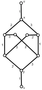
Please refer to Figure 1. Graph Qn, for n ≥ 3, is obtained from the
complete bipartite graph Kn,n by removing an edge xy, by adding new
pendant verticesu and v, and by adding pendant edges uxand vy. Graph Q′n is obtained from Qn by identifying vertices u and v into a vertex w.
Observe that Q′
n is a graph of maximum degree n, and has 2n+ 1 vertices
Figure 1: NP-complete gadgetQn and graphQ′n.
investigates the properties of graph Qn, which is used as “gadget” in the
NP-completeness proof of Theorem 2.
Lemma 1. Graph Qn is n-edge-colourable, and in any n-edge-colouring
of Qn, edges uxand vy receive the same colour.
Proof:
We use the notation from Figure 1. First, we exhibit ann-edge-colouring of Qn. Denote by x0, ..., xn−1 (resp. y0, ..., yn−1) the vertices of Qn which
belong to the same partition as x (resp. y), where x = x0 (resp. y = y0). An n-edge-colouring of Qn is constructed as follows: just let the colour of
edgexiyj be (i+j mod n) + 1 and let the colour of edgesx0uandy0vbe 1. Now we prove that, in anyn-edge-colouring ofQn, edgesuxandvyhave
the same colour. Suppose there is ann-edge-colouringπofQnwhereuxand
vy have different colours. Consider the graphQ′
n = (V′, E′) obtained from
Qn, by contracting vertices u and v into vertex w. Then we can construct
an n-edge-colouring π′ of Q′n by setting π′(e) = π(e) if e ∈ E′\ {ux, vy}, π′(wx) = π(ux) and π′(wy) = π(vy), which is a contradiction to the fact thatQ′
n is Class 2.
We prove in Theorem 2 the NP-completeness of edge-colouring regular graphs that do not contain a cycle with a unique chord for each fixed degree ∆≥3.
Theorem 2. For each∆≥3,CHRIND(∆-regular graph inC) is NP-complete.
Let G = (V, E) be an input of the NP-complete problem CHRIND
(∆-regular graph). Now, letG′ be the graph obtained fromGby removing each edge pq∈ E and adding a copy of Q∆, identifying verticesu and v of Q∆ with verticesp andq ofG. For each edgepqof G, denoteHpq the subgraph
of G′ isomorphic to Q
∆ whose pendant vertices are p and q. Observe that G′ is also ∆-regular.
Claim 1: G′ can be constructed in polynomial time from G. In fact, we make one substitution – by a copy of Q∆ – for each edge of G, so that the construction time is linear on the number of edges ofG.
Claim 2: if G is ∆-edge-colourable, then so is G′. Let π be a ∆-edge-colouring of G. We construct a ∆-edge-colouring π′ of G′ in the following way: for each edge pq of G, let the edges of Hpq in G′ be coloured in such
a way that the pendant edges have the colour π(pq) – this colouring exists and is described by Lemma 1.
Claim 3: if G′ is ∆-edge-colourable, then so is G. Let π′ be a ∆-edge-colouring ofG′. We construct a ∆-edge-colouring π of Gas follows: let the colour inπ of each edgepqof Gbe equal to the colour inπ′ of the pendant edges ofHpq (by Lemma 1, these two pendant edges must receive the same
colour).
Claim 4: G′ ∈ C. Suppose G′ has a cycle C with a unique chord αβ. Observe that, by construction, every edge of G′ – and, in particular, chord αβ – has both endvertices in the same copy of Q∆. Denote by Hp′q′ this
copy and observe that cycle C, when restricted to Hp′q′, is a path between
p′ and q′, and that αβ is a unique chord of this path. But there is no path with unique chord between the pendant vertices of Q∆, so that we have a contradiction.
Observe that graphG′ in the proof of Theorem 2 is tripartite with vertex tripartition (P1, P2, P3) determined as follows:
• P1 is the set whose elements are the original vertices of G and the vertices denotedy1, ..., y∆ in each copy ofQ∆;
• P2 is the set whose elements are the vertices denotedx0 andy0 in each copy ofQ∆;
• P3 is the set whose elements are the vertices denotedx1, ..., x∆in each copy ofQ∆.
So, the following result holds:
Theorem 3. For each k≥3,∆≥3, CHRIND(∆-regular k-partite graph) is
We emphasize thatC is a class with strong structure [26], yet, it is NP-complete for edge-colouring. We manage in Section 4 to define a subclass of Cwhere edge-colouring is solvable in polynomial time. Consider the classC′ as the subset of the graphs ofC that do not contain a square. The structure of graphs inC′ is stronger than that of graphs inC, and is described in detail in Section 3. Yet, the edge-colouring problem is still NP-complete for inputs inC′, as we prove next in Theorem 4. We recall that the proof of Cai and Ellis [5] for the NP-completeness of edge-colouring cubic square-free graphs generates a graph which has a cycle with unique a chord. In addition, remark that the gadget Q∆ used in the proof of the NP-completeness of edge-colouring graphs with no cycle with unique chord has a square. So, we need an alternative construction, which is based on the gadget ˜P shown in Figure 2. Graph ˜P is constructed in such a way that the identification of its pendant vertices generates a graph isomorphic toP∗, the graph obtained from the Petersen graph by removing one vertex. GraphP∗is a non-overfull Class 2 graph [6, 15]. The properties of ˜P with respect to edge-colouring are described in Lemma 2.
Figure 2: 3-edge-colouring of gadget graph ˜P .
Lemma 2. GraphP˜ is 3-edge-colourable, and in any 3-edge-colouring ofP˜, the edges uxand vy receive the same colour.
Proof:
Figure 2 shows a 3-edge-colouring of ˜P – observe that edgesuxand vy receive the same colour.
that gadget ˜P is used instead of Q∆.
Theorem 4. CHRIND(graph in C′ with maximum degree 3) is NP-complete.
Proof:
The proof is similar to that of Theorem 2, except that ∆ = 3 and gadget ˜
P is used instead of Q∆.
Observe that the graphG′ constructed in the proof of Theorem 4 is not regular. In fact, as we prove in Section 5.1, the edge-colouring problem can be solved in polynomial time if the input is restricted to cubic graphs ofC′.
3
Structure of graphs in
C
and
C
′The goal of the present section is to review structure results for the graphs inC and obtain stronger results for the subclass C′. These results are used in Section 4 to edge-colour the graphs inC′ with maximum degree at least 4. In the present section we review the results of Trotignon and Vuˇskovi´c [26] on the structure of graphs inC and obtain stronger results for graphs inC′. Let C be the class of the graphs that do not contain a cycle with a unique chord and letC′ be the class of the graphs ofC that do not contain a square. Trotignon and Vuˇskovi´c give a decomposition result [26] for graphs in C and graphs in C′ in the following form: every graph in C or in C′ either belongs to a basic class or has a cutset. Before we can state these decomposition theorems, we define the basic graphs and the cutsets used in the decomposition.
The Petersen graph is the graph on vertices {a1, . . . , a5, b1, . . . , b5} so that botha1a2a3a4a5a1 andb1b2b3b4b5b1 are chordless cycles, and such that the only edges between someai and somebi area1b1,a2b4,a3b2,a4b5,a5b3. We denote by P the Petersen graph and byP∗ the graph obtained fromP by removal of one vertex. Observe thatP ∈ C.
TheHeawood graphis a cubic bipartite graph on vertices{a1, . . . , a14}so thata1a2. . . a14a1 is a cycle, and such that the only other edges area1a10, a2a7,a3a12,a4a9,a5a14,a6a11,a8a13. We denote byH the Heawood graph and byH∗ the graph obtained from H by removal of one vertex. Observe thatH ∈ C.
For the purposes of this work, a graph Gis called basic1 if
1. G is a complete graph, a cycle-graph with at least five vertices, a strongly 2-bipartite graph, or an induced subgraph of the Petersen graph or of the Heawood graph; and
2. Ghas no 1-cutset, proper 2-cutset or proper 1-join (all defined next).
We denote byCB be the set of the basic graphs. Observe that CB ⊆ C.
A cutset S of a connected graph Gis a set of elements, vertices and/or edges, whose removal disconnectsG. A decomposition of a graph is the re-moval of a cutset to obtain smaller graphs, called theblocks of the decompo-sitions, by possibly adding some nodes and edges to connected components of G\S. The goal of decomposing a graph is trying to solve a problem on the whole graph by combining the solutions on the blocks. For a graph G= (V, E) and V′ ⊆V, G[V′] denotes the subgraph of G induced by V′. The following cutsets are used in the known decomposition theorems of the classC [26]:
• A 1-cutset of a connected graph G = (V, E) is a node v such that V can be partitioned into sets X, Y and {v}, so that there is no edge betweenX and Y. We say that (X, Y, v) is asplit of this 1-cutset.
• A proper 2-cutset of a connected graph G= (V, E) is a pair of non-adjacent nodesa, b, both of degree at least three, such that V can be partitioned into setsX,Y and {a, b}so that: |X| ≥2,|Y| ≥2; there is no edge betweenXandY, and bothG[X∪ {a, b}] andG[Y ∪ {a, b}] contain an ab-path. We say that (X, Y, a, b) is a split of this proper 2-cutset.
• A1-join of a graphG= (V, E) is a partition of V into setsX and Y such that there exist sets A, B satisfying:
– ∅ 6=A⊆X,∅ 6=B⊆Y;
– |X| ≥2 and |Y| ≥2;
– there are all possible edges betweenA and B;
– there is no other edge betweenX and Y.
1By the definition of [26], a basic graph is not, in general, indecomposable. However,
We say that (X, Y, A, B) is asplit of this 1-join.
A proper 1-join is a 1-join such that A and B are stable sets of Gof size at least two.
We can now state a decomposition result for graphs in C:
Theorem 5. (Trotignon and Vuˇskovi´c [26]) If G ∈ C is connected then eitherG∈ CB or G has a 1-cutset, or a proper 2-cutset, or a proper 1-join.
The block GX (resp. GY) of a graph G with respect to a 1-cutset with
split (X, Y, v) isG[X∪ {v}] (resp. G[Y ∪ {v}]).
The block GX (resp. GY) of a graph G with respect to a 1-join with
split (X, Y, A, B) is the graph obtained by taking G[X] (resp. G[Y]) and adding a node y complete to A (resp. x complete to B). Nodes x, y are calledmarkers of their respective blocks.
The blocks GX and GY of a graph Gwith respect to a proper 2-cutset
with split (X, Y, a, b) are defined as follows. If there exists a node c of G such that NG(c) = {a, b}, then let GX = G[X∪ {a, b, c}] and GY =
G[Y ∪ {a, b, c}]. Otherwise, block GX (resp. GY) is the graph obtained by
takingG[X∪ {a, b}] (resp. G[Y ∪ {a, b}]) and adding a new nodecadjacent toa, b. Nodec is a called themarker of the blockGX (resp. GY).
The blocks with respect to 1-cutsets, proper 2-cutsets and proper 1-joins are constructed in such a way that they remain inC, as shown by Lemma 3.
Lemma 3. (Trotignon and Vuˇskovi´c [26]) Let GX and GY be the blocks of
decomposition of G w.r.t. a 1-cutset, a proper 1-join or a proper 2-cutset. ThenG∈ C if and only if GX ∈ C and GY ∈ C.
We reviewed results that show how to decompose a graph ofC into basic blocks: Theorem 5 states that each graph in C has a 1-cutset, a proper 2-cutset or a proper 1-join, while Lemma 3 states that the blocks generated with respect to any of these cutsets are still in C. We now obtain similar results forC′. These results are not explicit in [26], but they can be obtained as consequences of results in [26] and by making minor modifications in its proofs. As we discuss in the following observation [4], for the goal of edge-colouring, we only need to consider thebiconnected graphs ofC′.
By Observation 1, if both blocksGX and GY are ∆(G)-edge-colourable,
then so isG. That is, once we know the chromatic index of the biconnected components of a graph, it is easy to determine the chromatic index of the whole graph. So, we may focus our investigation on the biconnected graphs ofC′.
Theorem 6. (Trotignon and Vuˇskovi´c [26]) If G∈ C′ is biconnected, then eitherG∈ CB or Ghas a proper 2-cutset.
Theorem 6 is an immediate consequence of Theorem 5: since G has no 4-hole,Gcannot have a proper 1-join, and sinceGis biconnected,Gcannot have a 1-cutset.
Next, in Lemma 4, we show that the blocks of decomposition of a bicon-nected graph ofC′ w.r.t. a proper 2-cutset, are also biconnected graphs of
C′. The proof of Lemma 4 is similar to that of Lemma 5.2 of [26]. For the sake of completeness, the proof, which uses the result of Theorem 7 below, is included here.
Theorem 7. (Trotignon and Vuˇskovi´c [26]) Let G ∈ C be a connected graph. If G contains a triangle then either G is a complete graph, or some vertex of the maximal clique that contains this triangle is a 1-cutset ofG.
Lemma 4. Let G∈ C′ be a biconnected graph and let (X, Y, a, b) be a split of a proper 2-cutset ofG. Then both GX andGY are biconnected graphs of
C′.
Proof:
We first prove that G is triangle-free. Suppose G contains a triangle. Then, by Theorem 7, either G is a complete graph, which contradicts the assumption thatGhas a proper 2-cutset, orGhas a 1-cutset, which contra-dicts the assumption thatGis biconnected. SoGis triangle-free, and hence by construction, both of the blocksGX and GY are triangle-free.
Now we show that GX and GY are square-free. Suppose w.l.o.g. that
GX contains a squareC. SinceGis square-free,C contains the marker node
M, which is not a real node of G, andC =M azbM, for some node z∈X. Since M is not a real node of G, we have degG(z) >2, otherwise, z would
be a marker of GX. Let z′ be a neighbor of z distinct of a and b. Since
So, by the minimality ofP, vertexbdoes not have a neighbor inP. Now let Qbe a path fromatobwhose interior is inY. So, bzz′P aQbis a cycle ofG with a unique chord (namelyaz), contradicting the assumption thatG∈ C. By Lemma 3, GX and GY both belong to C, and since GX and GY are
both square-free, it follows thatGX and GY both belong to C′.
Finally we show that GX and GY are biconnected. Suppose w.l.o.g.
that GX has a 1-cutset with split (A, B, v). Since G is biconnected and
G[X ∪ {a, b}] contains an ab-path, we have that v 6= M, where M is the marker ofGX. Supposev=a. Then, w.l.o.g.,b∈B, and (A, B∪Y, a) is a
split of a 1-cutset of G, with possiblyM removed from B∪Y, if M is not a real node of G, contradicting the assumption that G is biconnected. So v 6=a and by symmetry v 6= b. So v ∈X\ {M}. W.l.o.g. {a, b, M} ⊂B. Then (A, B∪Y, v) is a split of a 1-cutset of G, with possibly M removed fromB∪Y ifM is not a real node of G, contradicting the assumption that Gis biconnected.
Observe that Lemma 3 is somehow stronger than Lemma 4. While Lemma 3 states that a graph is in C if and only if the blocks with re-spect to any cutset are also inC, Lemma 4 establishes only one direction: if a graph is a biconnected graph of C′, then the blocks with respect to any cutset are also biconnected graph ofC′. For our goal of edge-colouring, there is no need of establishing the “only if” part. Anyway, it is possible to verify that, if both blocksGX andGY generated with respect to a proper 2-cutset
of a graph G are biconnected graphs of C′, then G itself is a biconnected graph ofC′.
Next lemma shows that every non-basic biconnected graph in C′ has a decomposition such that one of the blocks is basic.
Lemma 5. Every biconnected graphG∈ C′\ C
B has a proper 2-cutset such
that one of the blocks of decomposition is basic.
Proof:
By Theorem 6 G has a proper 2-cutset. Consider all possible 2-cutset decompositions of G and pick a proper 2-cutset S that has a block of de-compositionB whose size is smallest possible. By Lemma 4, B ∈ C′ and is biconnected. So by Theorem 6, eitherB has a proper 2-cutset or it is basic. We now show that in factB must be basic.
Let (X, Y, a, b) be a split w.r.t. S. Let M be the marker node of GX,
and assume w.l.o.g. thatB =GX. SupposeGX has a proper 2-cutset with
split (X1, X2, u, v). By minimality of B = GX, {a, b} 6= {u, v}. Assume
and hence (X1∪Y, X2, u, v), with M removed ifM is not a real node ofG, is a proper 2-cutset ofGwhose block of decompositionGX2 is smaller than GX, contradicting the minimality ofGX = B. Therefore a∈ {u, v}. Then
w.l.o.g. {b, M} ⊆X1, and hence (X1∪Y, X2, u, v), withM removed ifM is not a real node ofG, is a proper 2-cutset ofGwhose block of decomposition GX2 is smaller thanGX, contradicting the minimality ofGX =B. Therefore GX does not have a proper 2-cutset, and hence it is basic.
4
Chromatic index of graphs in
C
′with maximum
degree at least 4
The first NP-completeness result of Section 2 proves that edge-colouring is difficult for the graphs inC. We consider, further, the subclassC′ and verify that the edge-colouring problem is still NP-complete when restricted toC′. In the present section we apply the structure results of Section 3 to show that edge-colouring graphs inC′ of maximum degree ∆≥4 is polynomial by establishing that the only Class 2 graphs inC′ are the odd order complete graphs. Remark that the NP-completeness holds only for 3-edge-colouring restricted to graphs in C′ with maximum degree 3.
We describe, next, the technique applied to edge-colour a graph inC′ by combining edge-colourings of its blocks with respect to a proper 2-cutset. Observe that the fact that a graphF is isomorphic to a block B obtained from a proper 2-cutset decomposition ofGdoes not imply thatGcontains F: possibly B is constructed by the addition of a marker vertex. This is illustrated in the example of Figure 3, where G is P∗-free, yet, graph P∗ appears as a block with respect to a proper 2-cutset ofG.
The reader will also observe that it is not necessary that a block of decomposition ofG is ∆(G)-edge-colourable in order that Gitself is ∆(G)-edge-colourable: graph G in Figure 3 is 3-edge-colourable, while block P∗ is not. This is an important observation: possibly, the edges adjacent to a marker vertex of a block of decomposition are not real edges of the original graph, or are already coloured by an edge-colouring of another block, so that these edges do not need to be coloured.
Observation 2. Consider a graphG∈ C′ with the following properties:
• (X, Y, a, b) is a split of a proper 2-cutset of G;
• G˜Y is obtained from GY by removing its marker if this marker is not
Figure 3: Example of decomposition with respect to a proper 2-cutset{a, b}. Observe that the marker vertices and their incident edges – identified by dashed lines – do not belong to the original graph.
• π˜Y is a ∆(G)-edge-colouring of G˜Y;
• Fa (resp. Fb) is the set of the colours in {1,2, ...,∆} not used by π˜Y
in any edge ofG˜Y incident to a(resp. b).
If there exists a∆(G)-edge-colouringπX ofGX\M, whereM is the marker
vertex of GX, such that each colour used in an edge incident to a (resp. b)
is inFa (resp. Fb), then Gis ∆-edge-colourable.
The above observation shows that, in order to extend a ∆(G)-edge-colouring of ˜GY to a ∆(G)-edge-colouring of G, one must colour the edges
of GX \M in such a way that the colours of the edges incident to a (resp.
b) are not used at the edges of ˜GY incident toa(resp. b). This guarantees
that we create no conflicts. Moreover, there is no need to colour the edges incident to the markerM ofGX: if this marker is a vertex ofG, its incident
edges are already coloured by ˜π, otherwise, these edges are not real edges of G. In the example of Figure 3, we exhibit a 3-edge-colouring ˜πY of ˜GY. In
the notation of Observation 2,Fa={2,3}andFb ={2,3}. We exhibit, also,
a 3-edge-colouring ofGX\M such that the colours of the edges incident to
So, by Observation 2, we can combine colourings ˜πY and πX in a
3-edge-colouring ofG, as it is done in Figure 3.
Before we proceed and show how to edge-colour graphs in C′ with maxi-mum degree ∆≥4, we need to introduce some additional tools and concepts. A partial k-edge-colouring of a graph G= (V, E) is a colouring of a subset E′ ofE, that is, a functionπ :E′ → {1,2, ..., k} such that no two adjacent edges ofE′ receive the same colour.
Theset of free-coloursat vertexuwith respect to a partial-edge-colouring π:E′ →Cis the setC\π({uv|uv∈E′}). The list-edge-colouring problem is described next. Let G = (V, E) be a graph and let L = {Le}e∈E be a
collection which associates to each edgee∈E a set of colours Le called the
list relative toe. It is asked whether there is an edge-colouringπ ofGsuch that π(e) ∈ Le for each edge e ∈ E. Theorem 8 is a result on
list-edge-colouring which is applied, in this work, to edge-colour some of our basic graphs: strongly 2-bipartite graphs, Heawood graph and its subgraphs, and cycle-graphs.
Theorem 8. (Borodin, Kostochka, and Woodall [4]) Let G = (V, E) be a bipartite graph and L = {Le}e∈E be a collection of lists of colours which
associates to each edgeuv ∈Ea listLuvof colours. If, for each edgeuv∈E,
|Luv| ≥max{degG(u), degG(v)}, then there is an edge-colouringπ ofGsuch
that, for each edgeuv ∈E, π(uv)∈Luv.
We investigate, now, how to ∆(G)-edge-colour a graphG∈ C′ by com-bining ∆(G)-edge-colourings of its blocks with respect to a proper 2-cutset. More precisely, Lemma 6 shows how this can be done if one of the blocks is basic. Subsequently, we obtain, in Theorem 9, a characterization for graphs inC′ of maximum degree at least 4 of its Class 2 graphs which establishes that edge-colouring is polynomial for these graphs.
Lemma 6. Let G ∈ C′ be a graph of maximum degree ∆ ≥ 4 and let (X, Y, a, b) be a split of proper 2-cutset, in such a way that GX is basic. If
GY is ∆-edge-colourable, then Gis ∆-edge-colourable.
Proof:
Denote by M the marker vertex of GX and let ˜GY be obtained from
GY by removing its marker if this marker is not a real vertex ofG. Since
˜
GY is a subgraph ofGY, graph ˜GY is ∆-edge-colourable. Let πY be a
∆-edge-colouring of ˜GY, i.e. a partial-edge-colouring of G, and let Fa and
Fb be the sets of the free colours of a and b, respectively, with respect to
the partial edge-colouring πY. We show how to extend the partial
edges of GX \M. Since a and b are not adjacent, GX is not a complete
graph. Moreover, the blockGX cannot be isomorphic to the Petersen graph
or to the Heawood graph, because these graphs are cubic and GX has a
marker vertexM of degree 2. So, GX is isomorphic to an induced subgraph
ofP∗, or to an induced subgraph of H∗, or to a strongly 2-bipartite graph, or to a cycle-graph.
Case 1. GX is a strongly 2-bipartite graph.
Since degGX(M) = 2, vertexM belongs to the bipartition ofGX whose vertices have degree 2. So, verticesaand bbelong to the bipartition of GX
whose vertices have degree larger than 2, and |Fa| ≥ degGX\M(a) ≥2 and |Fb| ≥degGX\M(b)≥2. Associate to each edge ofGX\Mincident toa(resp. b) a list of colours equal toFa(resp. Fb). To each of the other edges ofGX\
M, associate list{1, ...,∆}. Now, to each edgeuv ofGX\M, a list of colours
is associated whose size is not smaller than max{degGX\M(u), degGX\M(v)} and, by Theorem 8, there is an edge-colouringπ1ofGX\M from these lists.
Finally, setπ :=π1 for the edges of GX\M.
Case 2. GX is a cycle-graph.
In this case, GX \ M is a path. Denote the vertices of GX \M by
a=x1, x2, ..., xk=b, in such a way thatx1x2...xk is a path. We now show
that k≥4. Sincea and b are not adjacent,k ≥3. Suppose thatk = 3. If M is a real node of G, then GX is a square and it is an induced subgraph of
G, contradicting the assumption that G is square-free. SoM is not a real node of G, and henceGX \M =X. But, then,|X|= 1, contradicting the
definition of a proper 2-cutset. Therefore,k≥4.
Observe that there is at least one colour cα in Fa and one colourcβ in
Fb. We construct a 3-edge-colouring π of CX \M by setting π(x1x2) :=cα
andπ(xk−1xk) :=cβ, and by colouring the other edges ofGX\M as follows.
If k= 4, let π(x2x3) be some colour in {1,2,3} \ {cα, cβ}, which is clearly
a non-empty set. Ifk≥5, letL2 ={L2, L3, ..., Lk−2} be a collection which associates to each edgexixi+1 a list of coloursLi such that:
• Li={1,2,3} \ {cα}, fori= 2,3, ..., k−3, and
• Lk−2={1,2,3} \ {cβ}.
Observe thatGX\ {M, a, b}is a path, hence bipartite of maximum degree 2,
and that|Li| ≥ 2 for each i= 2, ..., k−2, so that by, Theorem 8, there is
an edge-colouring π2 of GX \ {M, a, b} from the lists L2. Moreover, this colouring creates no conflicts with the colourscα of x1x2 and cβ of xk−1xk,
Observe thataandbhave onlyM as common neighbor inGX, otherwise
GX has a square (recall that Heawood graph is square-free). We construct a
4-edge-colouring ofGX\M. Denote the neighbors ofa(resp. b) inGX\Mby
a1, ..., ax (resp. b1, ..., by), wherex =degGX\M(a) (resp. y =degGX\M(b)). Note thatx, y∈ {1,2}. Observe thatFa(resp. Fb) contains at leastx(resp.
y) colours, which we denote by ca1, ..., cax (resp. cb1, cb2, ..., cby). Set the colourπ of edge aai (resp. bbj), fori= 1, ..., x(resp. for j= 1, ..., y), tocai (resp. cbj). Now, associate to each edge incident toai and different fromaai a list of colours{1,2,3,4} \ {cai}. Similarly, associate to each edge incident tobj and different ofbbj a list of colours{1,2,3,4} \ {cbj}. Finally, associate to each of the other edges of GX \ {M, a, b} the list of colours {1,2,3,4}.
Observe thatGX \ {M, a, b}is bipartite of maximum degree at most 3 and
that each of the lists has 3 or 4 colours, so that, by Theorem 8, there is an edge-colouringπ3 of GX\ {M, a, b}from these lists, and we setπ :=π3 for the edges ofGZ\M.
Case 4.a: GX =P∗.
Observe that there are at least two coloursca1, ca2 inFaand two colours cb1, cb2 inFb, and that exactly one of the following three possibilities holds:
• |{ca1, ca2} ∩ {cb1, cb2}|= 0;
• |{ca1, ca2} ∩ {cb1, cb2}|= 1; or
• |{ca1, ca2} ∩ {cb1, cb2}|= 2.
In the three cases, it is possible to extend the ∆-edge-colouringπY toG
by colouring the edges ofGX \M, as it is shown on Figure 4.
Case 4.b: GX is a proper induced subgraph ofP∗.
We need to investigate which are the proper induced subgraphs of P∗. We invite the reader to verify that, except for graph P∗∗ shown on the left of Figure 5, each proper induced subgraph of P∗ either has a 1-cutset or a proper 2-cutset, and we do not consider it becauseGX is assumed basic, or
is a cycle-graph, which is already considered in Case 2.
There is only one possible choice for the markerM ofGX =P∗∗, in the
sense that, for any other choice of markerM′, we haveG
X\M′ =GX\M.
As in Case 4.a, there are at least two colours ca1, ca2 inFa and two colours cb1, cb2 in Fb, and |{ca1, ca2} ∩ {cb1, cb2}|= 0, 1 or 2. In Figure 5 we exhibit three edge-colourings forP∗∗\M, one for each possibility.
Figure 4: Extending the colouring to the edges ofGX.
Figure 5: GraphP∗∗ and three edge-colourings of P∗∗\M subject to each possible free colour restriction.
Theorem 9. A connected graphG∈ C′ of maximum degree∆≥4is Class 2 if and only if it is an odd order complete graph.
Proof:
IfGis complete, then the theorem clearly holds. So, we prove that every connected graph of C′ that is not complete and whose maximum degree is at least 4 is Class 1. More precisely, we prove, by induction on the number of vertices, that, if ∆ is an integer at least 4 andG is a connected graph of C′ with maximum degree ∆(G)≤∆ and is not a complete graph on ∆ + 1 vertices, thenGis ∆-edge-colourable.
If G= (V, E) has four vertices or less, then ∆(G)≤3. Since ∆≥4, by Vizing’s theorem, graphGis ∆-edge-colourable.
[image:21.612.122.486.324.420.2]hypothesis, that every connected graph G′ ∈ C′ with k′ < k vertices such that ∆(G′) ≤ ∆ and G′ is not a complete graph on ∆ + 1 vertices, is ∆-edge-colourable. By Theorem 6 either Gis basic, orGhas a 1-cutset, or G is biconnected and has a proper 2-cutset.
Suppose G is basic. If G is strongly 2-bipartite, then G is ∆-edge-colourable because bipartite graphs are Class 1 and ∆(G) ≤ ∆. If G is not strongly 2-bipartite, then ∆(G)≤∆−1 andGis ∆-edge-colourable by Vizing’s theorem.
Now, suppose G has a 1-cutset with split (X, Y, v). Note that blocks of decompositionGX and GY are induced subgraphs ofG and hence both
belong to C′. By the induction hypothesis, both GX and GY are
∆-edge-colourable, and hence by Observation 1, graph Gis ∆-edge-colourable. Finally, supposeGis biconnected and has a proper 2-cutset. Let (X, Y, a, b) be a split of a proper 2-cutset such that blockGX is basic (note that such
a cutset exists by Lemma 5). By Lemma 4 block GY is in C′. By the
in-duction hypothesis, blockGY is ∆-edge-colourable. If ∆(G)≤3, then since
∆ ≥ 4, by Vizing’s theorem, G is ∆-edge-colourable. So we may assume that ∆(G)≥4, and hence by Lemma 6, Gis ∆-edge-colourable.
5
Graphs of
C
′with maximum degree 3
ClassC′has a stronger structure thanC, yet, edge-colouring problem is NP-complete for inputs in C′. In fact, the problem is NP-complete for graphs in C′ with maximum degree ∆ = 3. In this section, we further investigate graphs in C′ with maximum degree ∆ = 3, providing two subclasses for which edge-colouring can be solved in polynomial time: cubic graphs of C′ and 6-hole-free graphs of C′.
5.1 Cubic graphs of C′
In the present section, we prove the polynomiality of the edge-colouring problem restricted to cubic graphs of C′. This is a direct consequence of Lemma 7, which states that every non-biconnected cubic graph is Class 2, and Lemma 8, that states that the Petersen graph is the only biconnected cubic Class 2 graph inC′.
Lemma 7. Let G be a connected cubic graph. If G has a 1-cutset, then G is Class 2.
Denote by (X, Y, v) a split of a 1-cutset ofG. Observe thatvhas degree 1 in exactly one of the blocksGX andGY; assume, w.l.o.g. that this block is
GX. LetG′X be the graph obtained fromGX by removing vertexv. Observe
that G′X has exactly one vertex of degree 2 and each of the other vertices has degree 3. Since the sum of the degrees of the vertices is even, G′
X has
an even number of vertices of degree 3, sayn. So, the number of edges in G′X is (3n+ 2)/2. Since 3⌊(n+ 1)/2⌋ = 3n/2 < (3n+ 2)/2, graph G′X is overfull, so thatGis subgraph-overfull, hence Class 2.
Lemma 8. Let G ∈ C′ be biconnected graph. If G is cubic, then G is isomorphic to the Petersen graph or to the Heawood graph or is a complete graph on four vertices.
Proof:
Suppose G is not basic. By Lemma 5, G has a proper 2-cutset such that one of the blocks is basic. Let (X, Y, a, b) be a split of such cutset, in such a way thatGX is basic, and denote byM the marker vertex ofGX. If
degGX(a) = 1, vertexM is the only neighbor ofaand, clearly, is a 1-cutset of GX. By Lemma 4GX is a biconnected graph ofC′. SinceGX is biconnected
degGX ≥2. Leta
′ be a neighbor ofainG
X that is distinct fromM. Since
{M, a, b, a′}cannot induce a square,bis not adjacent toa′, and hence (since G is cubic) a′ has two neighbors in GX \ {a, b, M}. If degGX(a) = 2 then {a′, b} is a proper 2-cutset of G, contradicting the assumption that G
X is
basic. Hence degGX(a)≥3, and by symmetrydegGX(b)≥3. Observe that each of the other vertices – different froma, b and M – has degree ∆(G). In other words,GX is a graph with exactly one vertex of degree 2, and each
of the other vertices has degree 3. But there is no graph in CB with this
property, and we have a contradiction to the fact thatGX is basic. So,Gis
basic and the statement of the proposition clearly holds.
Theorem 10. Let G∈ C′ be a connected cubic graph. ThenG is Class 1 if and only if G is biconnected and is not isomorphic to the Petersen graph.
Proof:
If Gis not biconnected, then, by Lemma 7, G is Class 2. If Gis bicon-nected, then, by Lemma 8, thenG is isomorphic to the Petersen graph or to the Heawood graph or is a complete graph on four vertices. Hence,G is Class 2 if and only if it is isomorphic to the Petersen graph.
5.2 6-hole-free graphs of C′
Lemma 9, a variation for 3-edge-colouring of Lemma 6.
Lemma 9. Let G ∈ C′ be a graph of maximum degree at most 3 and (X, Y, a, b) be a split of a proper 2-cutset, in such a way that GX is basic
but not isomorphic to P∗. If GY is 3-edge-colourable, then G is
3-edge-colourable.
Proof:
AssumeGY is 3-edge-colourable. Denote byM the marker vertex ofGX
and let ˜GY be obtained from GY by removing its marker if this marker is
not a real vertex ofG. Since ˜GY is a subgraph ofGY, graph ˜GY is
3-edge-colourable. LetπY be a 3-edge-colouring of ˜GY, i.e. a partial-edge-colouring
ofG, and letFaandFb be the sets of the free colours ofaandb, respectively,
with respect to the partial edge-colouringπY. We show how to extend the
partial edge-colouring πY to G, as described in Observation 2, that is, by
colouring the edges ofGX \M. Sincea and b are not adjacent, GX is not
a complete graph. Moreover, the block GX cannot be isomorphic to the
Petersen graph or to the Heawood graph, because these graphs are cubic andGX has a marker vertexM of degree 2. Also, by assumption, block GX
is not isomorphic toP∗. So,GX is isomorphic to a proper induced subgraph
ofP∗, or to an induced subgraph of H∗, or to a strongly 2-bipartite graph, or to a cycle-graph.
Case 1. GX is a strongly 2-bipartite graph.
Similar to the Case 1 of the proof of Lemma 6, which also works for ∆ = 3.
Case 2. GX is a cycle-graph.
Similar to the Case 2 of the proof of Lemma 6, where at most three colours are used in the edges of GX \M.
Case 3. GX is an induced subgraph of H∗.
First, observe that degGX\M(a) = 2 anddegGX\M(b) = 2, otherwiseGX has a decomposition by a 1-cutset or a proper 2-cutset and is not basic. Observe, also, that there are at least two colours ca1, ca2 in Fa and two colourscb1, cb2 inFb, and that|{ca1, ca2} ∩ {cb1, cb2}|= 1 or 2. We consider each case next.
If |{ca1, ca2} ∩ {cb1, cb2}| = 1, we must exhibit a 3-edge-coloring π of GX\M such that the free colors ataandbare different. IfM is a real node
of G, thenGX is an induced subgraph of G, and hence ∆(GX) ≤3. If M
is not a real node of G, then by definition of proper 2-cutset both aand b have a neighbor in Y, and hence ∆(GX)≤3. So ∆(GX)≤3. Since GX is
bipartite,GX has a 3-edge-colouringπ′. So, letπ be the restriction of π′ to
If|{ca1, ca2} ∩ {cb1, cb2}|= 2, we must exhibit a coloring ofGX\M such that the free colors ataand bare the same. We exhibit these colourings for each possible induced subgraph of the Heawood graph. First, consider the caseGX =H∗, whose coloring is given in Figure 6.
Figure 6: A 3-edge-colouring of H∗ \M such that the sets of the colours incident to vertex aand vertexb are the same.
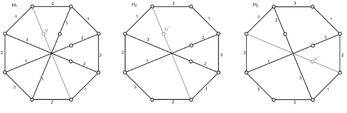
Now, observe that each non-basic proper subgraph of H∗ is a subgraph of the graph H1 of Figure 7, which is obtained from H∗ by removing a vertex of degree 2. GraphH2 of Figure 7 is obtained fromH1 by removing one of the four vertices of degree 2 (any choice yields the same graph up to an isomorphism). Finally, the last non-basic proper subgraph of H∗ is the graphH3 of Figure 7. Observe that there is only one possible choice M for
Figure 7: Non-basic proper induced subgraphs ofH∗
[image:25.612.144.465.481.579.2]edge-colouring ofH1\M, and two edge-colourings ofH2\M, one for each possible choice of marker M. We don’t consider here that case GX = H3
Figure 8: 3-edge-colourings ofH1 andH2, for each possible choice of marker.
becauseH3 is a strongly 2-bipartite graph, considered in Case 1. Case 4. GX is a proper subgraph ofP∗.
As we already discussed in Case 4 of Lemma 6, except for graph P∗∗ shown on the left of Figure 5, each of the other proper induced subgraphs of P∗ either has a 1-cutset or a proper 2-cutset, and we do not consider because GX is basic, or is a cycle-graph, which are considered in Case 2.
There is only one possible choice of markerM1for the caseGX =P∗∗, in the
sense that for any other choice of markerM′
1, we haveGX\M1′ =GX\M1. Observe, also, that there are at least two colours ca1, ca2 in Fa and two colours cb1, cb2 in Fb, and that |{ca1, ca2} ∩ {cb1, cb2}|= 1 or 2. These two possibilities are considered in the first two colourings of Figure 5.
Remark that the NP-Complete gadget ˜P of Figure 2 is constructed from P∗. The NP-completeness of edge-colouring graphs in C′ is obtained as a consequence of P∗ ∈ C′. Using Lemma 9, we can prove that if the special graph P∗ does not appear as a leaf in the decomposition tree, i.e., as a basic block when we recursively apply the proper 2-cutset decomposition to a biconnected graphG∈ C′ of maximum degree 3, thenG is Class 1.
Theorem 11. Let G ∈ C′ be a connected graph of maximum degree 3. If G does not contain a 6-hole all of whose nodes are of degree 3, then G is Class 1.
Suppose G is basic. G cannot be strongly 2-bipartite nor an induced subgraph of Heawood graph, since bipartite graphs are Class 1 [29]. G cannot be a complete graph on four vertices, beacuse such a graph is 3-edge-colourable. G cannot be a hole since it has maximum degree 3. So G must be an induced subgraph of the Petersen graph. Gcannot be isomorphic toP norP∗, because both of these graphs contain a 6-hole all of whose nodes are of degree 3. But all the other induced subgraphs of the Petersen graph are in fact 3-edge-colourable. ThereforeGcannot be basic.
Now suppose thatGhas a 1-cutset with split (X, Y, v). Note that blocks of decomposition are induced subgraphs ofG, and hence both are connected graphs of C′ that do not contain a 6-hole all of whose nodes are of degree 3. If ∆(GX) = 3 then since G is a minimum counterexample, GX is
3-edge-colourable. If ∆(GX) ≤ 2 then GX is 3-edge-colourable by Vizing’s
Theorem. SoGX is 3-edge-colourable, and similarly so is GY. But then by
Observation 1,G is also 3-edge-colourable, a contradicion.
Therefore G is biconnected and has a proper 2-cutset. Let (X, Y, a, b) be a split of a proper 2-cutset such that blockGX is basic (note that such
a cutset exists by Lemma 5). By Lemma 4 both of the blocksGX and GY
are biconnected graphs of C′. Since the marker node M is of degree 2 in both GX and GY, and GX \M and GY \M are both induced subgraphs
of G, it follows that neither GX nor GY can contain a 6-hole all of whose
nodes are of degree 3. IfM is a real node of G, then GX and GY are both
induced subgraphs of G, and hence ∆(GX) ≤ 3 and ∆(GY) ≤ 3. If M is
not a real node of G, then by definition of proper 2-cutset both a and b have a neighbor in both X and Y, and hence ∆(GX)≤3 and ∆(GY)≤3.
Since both GX and GY have fewer nodes than G, it follows either from
minimality of counterexampleGor by Vizing’s Theorem that bothGX and
GY are 3-edge-colourable. Since GX does not contain a 6-hole all of whose
nodes are of degree 3,GX is not isomorphic to P∗, and hence by Lemma 9,
Gis 3-edge-colourable, a contradiction.
Corollary 1. Every connected 6-hole-free graph of C′ with maximum de-gree 3 is Class 1.
A natural question in connection with Theorem 12 is whether forbidding 6-holes would make it easier to edge-colour graphs ofC′, and the answer is
no. By observing graphG′ of the proof of Theorem 2, one can easily verify that this graph has no 6-hole, so that the following theorem holds:
Theorem 12. For each∆≥3,CHRIND(∆-regular 6-hole-free graph inC) is
References
[1] M. M. Barbosa, C. P. de Mello, and J. Meidanis. Local conditions for edge-colouring of cographs. Congr. Numer.133 (1998) 45–55.
[2] H. L. Bodlaender. Polynomial algorithms for graph isomorphism and chromatic index on partial k-trees. J. Algorithms 11(1990) 631–643.
[3] V. A. Bojarshinov.Edge and total colouring of interval graphs. Discrete Appl. Math. 114(2001) 23–28.
[4] O. V. Borodin, A. V. Kostochka, and D. R. Woodall. List edge and list total colourings of multigraphs. J. Combin. Theory Ser. B71(1997) 184–204.
[5] L. Cai and J. A. Ellis.NP-Completeness of edge-colouring some restricted graphs. Discrete Appl. Math.30(1991) 15–27.
[6] D. Cariolaro and G. Cariolaro.Colouring the petals of a graph. Electron. J. Combin.10 (2003) #R6.
[7] B. L. Chen, H.-L. Fu, and M. T. Ko.Total chromatic number and chro-matic index of split graphs. J. Combin. Math. Combin. Comput. 17 (1995) 137–146.
[8] C. M. H. de Figueiredo, J. Meidanis, C. P. de Mello, and C. Ortiz. Decom-positions for the edge colouring of reduced indifference graphs. Theoret. Comput. Sci.297 (2003) 145–155.
[9] C. M. H. de Figueiredo, J. Meidanis, and C. P. de Mello.Local conditions for edge-coloring.J. Combin. Math. Combin. Comput.32(2000) 79–91.
[10] C. De Simone and C. P. de Mello.Edge-colouring of join graphs. The-oret. Comput. Sci.355 (2006) 364–370.
[11] C. De Simone and A. Galluccio. Edge-colouring of regular graphs of large degree. Theoret. Comput. Sci.389 (2007) 91–99.
[12] A. Gy´arf´as.Problems from the world surrounding perfect graphs. Zastos. Mat. 19(1987) 413–441.
[14] D. S. Johnson.The NP-completeness column: an ongoing guide. J. Al-gorithms6 (1985) 434–451.
[15] A. J. W. Hilton and Cheng Zhao. On the edge-colouring of a graph whose core has maximum degree two. J. Combin. Math. Combin. Com-put. 21(1996) 97–108.
[16] A. G. Chetwynd and A. J. W. Hilton.Star multigraphs with three ver-tices of maximum degree. Math. Proc. Cambridge Philos. Soc.100(1986) 303–317.
[17] D. G. Hoffman and C. A. Rodger. The chromatic index of complete multipartite graphs. J.Graph Theory 16(1992) 159–163.
[18] D. Leven and Z. Galil.NP-completeness of finding the chromatic index of regular graphs. J. Algorithms 4 (1983) 35–44.
[19] R. C. S. Machado and C. M. H. de Figueiredo.Decompositions for edge-coloring join graphs and cobipartite graphs. To appear in Discrete Appl. Math.
[20] T. Niessen. How to find overfull subgraphs in graphs with large maxi-mum degree. II.Electron. J. Combin. 8 (2001) #R7.
[21] C. Ortiz, N. Maculan, and J. L. Szwarcfiter.Characterizing and edge-colouring split-indifference graphs. Discrete Appl. Math.82(1998) 209– 217.
[22] M. Plantholt. The chromatic index of graphs with a spanning star. J. Graph Theory5 (1981) 45–53.
[23] B. Randerath and I. Schiermeyer. Vertex colouring and forbidden subgraphs—a survey. Graphs Combin.20 (2004) 1–40.
[24] D. P. Sanders and Y. Zhao. Planar graphs of maximum degree seven are class I. J. Combin. Theory Ser. B83(2001) 201–212.
[25] E. Steffen. Classifications and characterizations of snarks . Discrete Math. 188(1998) 183–203.
[27] V. G. Vizing. On an estimate of the chromatic class of a p-graph (in russian). Diskret. Analiz3 (1964) 25–30.
[28] V. G. Vizing. Critical graphs with given chromatic index (in russian). Diskret. Analiz 5 (1965) 9–17.