Multi-View Pedestrian Detection using Statistical Colour Matching

Multi-View Pedestrian Detection using Occupancy

Color Matching

Jie Ren

College of Electronics and Information

Xi’an Polytechnic University Xi’an, Shaanxi 710048, P. R. China

Email: renjie [email protected]

Ming Xu

Department of Electrical and Electronic Engineering Xi’an Jiaotong-Liverpool University Suzhou, Jiangsu 215123, P. R. China

Email: [email protected]

Jeremy S. Smith

University of Liverpool Liverpool, L69 3BX, UK Email: [email protected]

Abstract—To increase the robustness of detection in intelligent video surveillance systems, homography has been widely used to fuse foreground regions projected from multiple camera views to a reference view. The objective of this paper is to detect multiple pedestrians and identify the false-positive detections, which occur due to the foreground intersections of non-corresponding objects, in the top view using occupancy information and colour matching. Multiple homographies are used to detect the head plane and height of each pedestrian. The head locations can be used in the further tracking part. Experimental results show good performance of this method. This method can overcome the problems in the single color matching approach.

I. INTRODUCTION

Intelligent visual surveillance is an active research area in artificial intelligence and computer vision. The aim of an intelligent visual surveillance system is to detect, track, classify objects and recognize events automatically. Detecting multiple pedestrians is a challenging task in video surveillance, because of the occlusion between people in the scene. Using multiple cameras is a reasonable method to solve occlusions, because when an object is occluded in one view, it may be visible in the other camera views. Furthermore, the multiple camera views can extend the overall field of view.

To associate camera views and to fuse information from all the camera views, one useful assumption is that in all camera views the objects of interest are on a common plane. This assumption is valid for most scenarios in intelligent visual surveillance systems. Then, homography, a geometric transformation which shows a pixelwise mapping between two views according to a common plane, can be used as an efficient method to associate multiple camera views. Using a homography transformation, foreground regions detected from each of the multiple camera views can be projected to a reference view according to the homography for a specific plane. The intersection regions of the foreground projections indicate the locations of moving objects on that plane. This method achieved good results in detection and is robust in coping with occlusion.

This paper proposed a method to detect multiple pedestrians. Multiple homographies are used to detect the head plane and height of each pedestrian. To identify the false-positive detections, which occur due to the foreground intersections

of non-corresponding objects in the top view, the occupancy information and colour matching are applied in head plane detection.

The remainder of this paper is organized as follows: In Section II, the related work is discussed. Section III briefly describes the techniques used to estimate the homographies for the ground plane and a set of parallel head planes. In Section IV, the algorithms for detecting foreground regions and approximating each region with a polygon are discussed. In Section V, after the fusion of the multiview foreground regions is introduced, the approach based on the occupancy information and colour cue for multiple pedestrian detection is presented. The experimental results are discussed in Section VI, followed by the conclusions.

II. RELATEDWORK

As using multiple cameras in a visual surveillance system can provide a larger overall field of views and can reduce occlusions in the overlapping field of view, one of the key issues for visual surveillance with multiple cameras is how to utilize the information from the multiple cameras for the purpose of detection and tracking. The more information from the multiple cameras which can be used simultaneously, the more robust and accurate the system becomes. Depending on the degree of information fusion, the existing multi-camera surveillance systems can be categorized as low-degree in-formation fusion, intermediate-degree inin-formation fusion and high-degree information fusion.

The first category of the visual surveillance systems uses multiple cameras to extend the limited field of view for a single camera [1]–[4]. It is known as the camera handoff method which starts tracking objects with a single camera view and switches to the next camera when the tracked object goes beyond the field of view (FOV) of the current camera. For the camera handoff method, existing research differ on three points: when the handoff process is triggered, which camera will be selected as the next optimal camera to track and monitor the object of interest and how to establish the correspondence of the objects between the cameras.

camera when the system predicts that the current camera will no longer have a good view. The features extracted from the upper human bodies are used to build the object correspondence between cameras. The next camera should not only provide the best view but also have the least switching to continue tracking in that camera view.

In [2], the edges of the field of view of each camera, which can be seen in other cameras, are defined as field of view lines. The field of view lines are used to establish the correspondence of trajectories between cameras. The camera handoff is triggered when the object becomes too close to the edge of the cameras field of view (EFOV). However, the authors did not give quantitative values of what is considered as too close to the EFOV and which camera is the most qualified camera to track the handoff object.

In these approaches, the detection and tracking are applied in separate cameras, and only one camera is actively working at a particular time stamp. Therefore, it fails to detect and track objects during dynamic occlusions as this is one of the problems with single-camera visual surveillance systems. Since there is very limited information exchange between the cameras, this camera switch approach is classed as a low-degree information fusion method.

If the correspondence of the objects between cameras is established, it is possible to not only track objects as they move from one camera view to the other, but also to robustly align the trajectories in multiple views and fuse them for a improved tracking result. Khan and Shah [5] extended their work proposed in [2] by creating associations across views for a better localization of the object. The trajectories from each camera are fused into the reference view if that camera view can be visible in the reference view. In [6], the authors align the multiple views with the viewpoint of the camera which can give a clear view of the scene and fuse the trajectories from multiple views in that view. In [16], the multiview process uses Kalman trackers to model the object position and velocity, to which the multiple measurements input from the single-view stage are associated.

In addition to the tracking data, extracted features in indi-vidual camera views can be integrated into a reference view to obtain a global estimation. The extracted features include bounding boxes, centroids, principal axes and classification results. In [7], a motion model and an appearance model of each detected moving object are built. Then the moving objects are tracked using a joint probability data association filter in a single camera view. The bounding boxes of the moving objects are projected to a reference view according to the ground-plane homography to correct falsely detected bounding boxes and handle occlusions in the reference view. Du and Piater [8] use particle filters to track targets in the individual camera views and then project the principal axes of the targets onto the ground plane. After tracking the intersections of the principal axes using the particle filter on the ground plane, the tracking results are warped back into each camera view to improve the tracking in the individual camera views. Hu et al. Hu et al. [9] also project the extracted centre principal axes

of each foreground object from the individual camera views to a top view according to the homography mapping for the ground plane. The foot point of each object in the top view is determined by the intersection of the axes projections from two camera views. The tracking is based on the foot point locations in the top view. In [10] global tracking is based on the intersections of the 3D lines, in which the centroids of the tracking targets are mapped from multiple views to 3D lines in terms of the world coordinates.

These methods are grouped into the intermediate-level in-formation fusion category of the multiview methods. Although these methods attempt to resolve dynamic occlusions through the integration of information from additional cameras as occlusions might not occur simultaneously in all the cameras viewing an object, they are still vulnerable to occlusion. The reason is that features are extracted from the individual camera views before fusion, and problems that arise in the detection and tracking with a single camera will affect the final fusion result.

In recent years a third category of multiview methods has emerged, in which the individual cameras no longer extract features but provide foreground bitmap information to the fusion centre. The objects are detected as the visual hull intersections of these foreground bitmaps from multiple views. In [11], homography mapping is used to combine fore-ground likelihood images from different views to resolve occlusions and determine regions on the ground plane. In [12] and [13] , the midpoints of the matched foreground segments in each pair of cameras are back-projected to yield points in the 3D world. These points are then projected onto the ground plane to generate the probability distribution map of the object locations. Berclaz, Fleuret and Fua [14] divided the ground plane into grids to calculate the occupancy map in the ground plane. The probability that each sub-image corresponds to the average size of a person in each camera view is warped from each camera view to the top view for the ground-plane homographies independently.

The ground plane was later extended to a set of planes parallel to, but at some height off the ground plane to reduce false positives and missed detections [15]. In [16], a similar procedure was followed but the set of parallel planes are at the height of peoples heads. This method is able to handle highly crowded scenes because the feet of a pedestrian are more likely to be occluded in a crowd than the head. Their work achieves good results in moderately crowded scenes. The third category fully utilizes the visual cues from multiple cameras and has high-level information fusion.

III. HOMOGRAPHYESTIMATION

Planar homography is a special relationship, defined by a 3×3 transformation matrix H between a pair of captured images of the same plane with different cameras. Let (x, y) and (x0, y0) be a pair of corresponding points on that plane in the two images. x = [x, y,1]T _{and x}0 _{= [x}0_{, y}0_,1]T _are

associated by the homography matrix H:

x0∼=Hx (1)

where ∼= denotes that the homography is given up to an unknown scalar.

A. Estimation of the Ground Plane Homography

Homographies are usually estimated between a pair of images by finding feature correspondence in these images. As the homography transformation is a special variation of the projective transformation, the parameters recovered in the camera calibration can be used to determine the homography matrix for the ground plane. Let x = [xs, ys,1]T be a point

in the image without distortion andX= [Xw, Yw, Zw,1]Tbe

the point in the 3D world, the relationship that maps Xtox

can be rewritten using a 3×4projection matrix M:

x=MX=m1 m2 m3 m4X (2)

By assuming that the points X and x are on the ground plane, the pointXon the ground planegin the 3D world can be denoted asXg= [Xw, Yw,1]T, whereZw= 0is removed.

The ground-plane homography Hg can be denoted as:

Hg=

m1 m2 m4 (3)

B. Estimation of Multi-Plane Homographies

Homography mapping is not limited to the homography for the ground plane, and can be extended to a set of planes parallel to the ground plane and at some height. If the camera is calibrated, the multi-plane homographies can be calculated through the parameters recovered in the calibration process directly. For a plane p at some heighth, since the result, in which each element in the third columnm3multiples the value Zw=hinX, is a constant value and the last element in the

homogrenous vector X is 1, according to the homography projection for plane p, the projection from point Xin the 3D world to pointxin the 2D image is:

x=HpX=

m1 m2 m4+hm3X (4)

The homography of planepcan be represented as a combi-nation of the homography for the ground plane and the third column of the projection matrix M multiplied by a given height h:

Hp=Hg+

0 |hm3

(5)

where[0]is a3×2 zero matrix [17] .

IV. FOREGROUNDPOLYGON

As an essential process in visual surveillance systems, foreground segmentation aims to separate moving objects from a background image in each frame. The background subtraction method involves calculating a background image, subtracting each new frame from the background image and thresholding the subtraction result. Since the foreground pixels are identified according to the pixelwise difference between the new frame and the background image, the method is highly dependent on a good background model, which should not

be sensitive to illumination variations, shadows and waving vegetation. The MoG model is the most widely used method to cope with switching background elements (e.g., waving trees). According to the assumption that a background pixel is more stable than a foreground pixel in pixel values, the value of a background pixel is modelled by using a mixture of Gaussian distributions. The sum of the probability density functions weighted by the corresponding priors represents the probability that a pixel is observed at a particular intensity or colour [18].

After the foreground pixels in each single camera view are detected, these pixels need to be grouped into foreground regions by applying connected component analysis, morpho-logical operations and a size filter.

Once the foreground regions have been identified in a camera view, each foreground region need to be projected to a reference view according to the homography for a certain plane. As a pixelwise homographic transformation is time consuming, each foreground region is approximated by the polygon of the foreground region’s contour [19]. The Douglas-Peucker (DP) method [20] has been used for the polygon approximation. Instead of applying the inverse homography to each pixel in the reference view, the vertices of the polygon of each detected foreground region are projected to a reference view through homography mapping.

V. MULTIPLEPEDESTRIANDETECTION

When the foreground regions for the same object are warped from multiple views to the top view, they will intersect at a location where the object touches the ground. Although the ground plane is the most commonly used plane in homogra-phy mapping, the foreground projections of the same object, each from one of multiple camera views, may have missed intersections in the reference view. This may happen in at least three scenarios. Firstly, pedestrians’feet are quite small objects and are frequently missed in detection, when a pedestrian is striding and hence has their two legs separated. Furthermore, their feet are not necessarily touching the ground while they are walking.

Fig. 1. A schematic diagram of the foreground projection according to the homographies.

as the location of a person’s head top. The heigh of its corresponding plane indicates the height of that person.

A. Region Based Foreground Fusion

After the vertices of the foreground polygons are projected onto the reference image, the foreground regions are then rebuilt by filling the internal area of each polygon with a fixed value. Let plane p be a head plane and Fa

i be the i-th

foreground detection in the cameraa, its projected foreground region in the top viewtaccording to the homagraphy for plane pcan be described as:

F_i,pa,t=Ha,t_p (F_ia) (6)

Fig.1 shows a schematic diagram of the homography pro-jection according to the ground plane and a head plane parallel to the ground plane. Plane pis an imaginary plane parallel to the ground plane g at the height of a person’s head.

Let F_j,pb,t be thej-th projected foreground regions from the camera viewsbto the top view according to the homographies Hpb,t for the head plane. These foreground projections are

overlaid in the top view. If the two projected foreground regions from each of the two camera views intersect in the top view, these two projected foreground regions in the top view and their original foreground regions in each camera view are defined as a pair of projected foreground regions. The intersection region of the projected foreground regions F_i,pa,t andF_j,pb,t is denoted as:

Pi,j,pt =F a,t i,p ∩F

b,t

j,p (7)

B. Phantoms

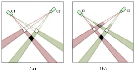
When the foreground images in the individual camera views are projected into the top view according to the homography for the ground plane or a plane parallel to the ground plane and at some height, the foreground regions from the different camera views may intersect in the top view, in which the intersections indicate the regions which may contain objects. If the intersecting foreground regions from the different camera views correspond to the same object, the intersection region reports the location where the object touches the plane used in the homography projection. If the intersection regions are caused by non-corresponding foreground regions from different camera views, they are false positive detections or phantoms. This is an important problem in multi-camera mov-ing object detection usmov-ing foreground homography mappmov-ing.

(a) (b)

Fig. 2. A schematic diagram of the homography mapping according to the ground-plane and planep.

Fig.2 is a schematic diagram which illustrates how non-corresponding foreground regions intersect and give rise to a false-positive detection in homography mapping. The warped foreground region of an object in the top view is observed as the intersection of the ground plane and the cones swept out by the silhouette of that object. When the foreground regions for the same object are warped from multiple views to the top view, they will intersect at the location where the object touches the ground. However, if the warped foreground regions from different objects intersect in the top view, the intersection region will lead to a phantom detection. In Fig.2(a), the fore-ground regions of two objects are projected from two camera views into the top view. The foreground projections intersect in three regions on the ground plane. The white intersection regions are the locations of the two objects, whilst the black region may be a phantom. Utilizing homography mapping for a plane higher than the ground plane can cause additional phantoms. The reason for this is that the projected foreground regions are moving to the camera. A schematic diagram of the foreground projection according to the homographies for the ground plane and a plane parallel to and off the ground plane is shown in Fig.1. Compared with the foreground projection on plane g, the projected foreground region on head plane p moves towards the camera. When such projected foreground regions on the plane off the ground intersect those from other camera views in the top view, additional phantoms may be generated. A schematic diagram of the homography mapping according to planep is shown in Fig.2(b), in which the grey region is an additional phantom.

C. Occupancy Calculation

If the intersection region P_i,j,pt is formed by an object, it indicates the location of where the object is intersected by plane p. When plane p is at different heights and parallel to the ground plane, the intersection region Pt

i,j,p varies in

its size and shape, which approximates the widths of the corresponding body parts at different heights.

(a) (b) (c)

(d) (e) (f)

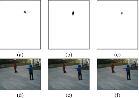
Fig. 3. An example of the projected foreground intersections due to the same object by using the homographies for a set of planes at different heights. (a), (b) and (c) are the intersection region in the top view for the ground plane, the plane at heights of1.0mand1.5m, (d), (e) and (f) are the warped back region in camera viewbfor the ground plane, the plane at at heights of1.0m

and1.5m.

shows the location of that object intersected by that plane. Fig.3(a) shows the intersection region according to the ho-mography for the ground plane. Such an intersection region is then warped back into a single camera view (Fig.3(d)), where the green lines and red dots represent the polygon edges and vertices of the back-warped intersection region in camera view b. Fig.3 (b)(c)(e)(f) show the results at heights of 1.0m and 1.5m.

Assuming that the pedestrians are standing upright, the ground plane g and the head plane p are considered. The intersection region Pt

i,j,g and Pi,j,pt are roughly at the same

position in the top view(see Fig.3(a) and (c)). Let It

i,j,p(x, y)

be a pixel in Pt

i,j,p in the top view. If Pi,j,pt is occupied

by an real object, when the pixel is warped back to camera view c according to the head plane homography Ht,c

p , the

warped back pixel I_i,j,pt,c is located around the head area of the corresponding foreground region in camera view c. When the pixel is warped back to the individual camera view according to the ground plane homography Ht,c

g , the

warped back pixelI_i,j,gt,c is located around the foot area of the corresponding foreground region in camera view c. Pixels on the line which is decided by those two warped back pixels are located inside the corresponding foreground region in the camera view. However, if Pt

i,j,p is a phantom region, the

warped back pixels I_i,j,pt,c and I_i,j,gt,c are not located around the head area or food area of their corresponding foreground region in the individual camera view. Some pixels on the line which is decided by those two warped back pixels are located outside its corresponding foreground region in the camera view. Therefore, the percentage which pixels are on the line decided by two warped back pixels and inside its corresponding foreground region indicates the likelihood that the original pixel in the top view belongs to an real object. That likelihood is donated asLt,c

p (x, y).

Instead of filling the intersection region with a fixed value,

individual pixel in the intersection region is marked with its likelihoods from all camera views.

Lt_i,j,p(x, y) =Y

C

Lt,c_i,j,p(x, y) (8)

When the likelihood of each pixel in the intersection regions in the top view is calculated, the occupancy map likelihood that the intersection regions are occupied by real objects is generated.

D. Colour Matching

Since colour is a strong cue to differentiate objects, the colours of the warped back intersection regions in individual camera views are utilized to identify whether two foreground projections from different camera views are due to the same object. Pixelwise colour matching is sensitive to homography estimation errors. It also assumes that each foreground region of the same object has consistent colour patterns in the different camera views. In reality, because multiple cameras are often placed at different orientations, the same object may appear slightly different in the colour patterns in the different camera views. Therefore, pixelwise colour matching cannot achieve good results in these situations and a statistical approach based on the colour cue is proposed.

The colour statistical approach is not based on the warped colour patches in the top view, because the warping operation may change the statistical properties of a colour patch. This approach is based on the original colour patches in the two camera views, which correspond to the same foreground intersection region in the top view. A pair of such colour patches often have different sizes. Each intersection region in the top view needs to be warped back to the individual camera views firstly. Given an head-plane intersection regionPt

i,j,p in

the top view, the image patch in camera view a, which is warped back from the top view using the homography for a planep, which parallel to the ground plane and athi,jheight,

is as follows:

P_i,j,pa = (Ha,t_p )−1P_i,j,pt (9) Then, the color model of the warped back patch is built by using the colors of all the pixels in that patch. The Gaussian mixture model is applied to handle the multiple colors in the warped back patch. Ifxi is theddimensional color vector of

a pixel in the torso region, the color vectors of N pixels are denoted byX={xi}Ni=1. LetK be the number of Gaussian

distributions used in the Gaussian mixture model, the Gaussian mixture model is denoted as:

p(xi) = K X

k=1

πkN(xi|µk, σk) (10)

The K-means algorithm and the Expectation-maximization (EM) algorithm are widely used to find the parameters of the probability density functions in a Gaussian mixture model. For the warped back patchPa

i,j,p, the color of that patch is modeled

by K Gaussian distributions: N(πa

whereπa_i,n,µa_i,nandσa_i,nare the weight, mean and covariance of then-th Gaussian distribution. TheKGaussians are ordered according to the magnitudes of the weights and πa

i,1 is the

greatest weight.

Let P_i,j,pb be the warped back patch in the camera view b using the homography for a plane p parallel to the ground plane and athi,jheight, the color of that patch is modeled by

K Gaussian distributions: N(πb

i,m, µbi,m, σbi,m), m ∈ [1, K],

whereπb

i,m,µbi,m andσi,mb are the weight, mean and

covari-ance of the m-th Gaussian distribution. The color similarity of those warped back patches, which correspond to the same intersection region in the top view, is measured according to the Mahalanobis distance of those two color models. Since the Gaussian distributions in each GMM are ranked in a descending order, the first distribution is always the dominant distribution in the GMM. In the first step, the Mahalanobis distances between the dominant distributionN(πa

i,1, µai,1, σai,1)

and each of the significant distributions:

cai,j,m= (µai,1−µbi,m)T(σi,a1+σi,mb )−1(µai,1−µbi,m) (11)

When the Mahalanobis distances between the dominant distribution and all the significant distributions are calculated, which are donated as ca

i,j and cbi,j, the minimum value is

thought of as the colour distance between the pair of colour appearance models:

ca,b_i,j =min(ca_i,j∩cb_i,j) (12)

E. Head Intersection

Assuming that the pedestrians are standing upright and the height of pedestrians are various, theDvirtual planes at differ-ent heights are considered. Lethbe the height of planepwith a height range [1.5m,1.8m].Pt

i,j,p (p∈[1.5,1.8])represent a

set of foreground intersection regions at different heights but at the same location in the top view. The intersection which has the highest height and its occupancy likelihood is higher than a threshold, color matching result is lower than a threshold, area is over a threshold is recognized as the location of a person’s head top. The heigh of its corresponding plane indicates the height of that person. The satisfied intersection regions indicate the location of pedestrians.

VI. EXPERIMENTALRESULTS

The algorithm has been tested on a dataset which was captured in the author’s campus. Two cameras were placed with small viewing angles and with significant overlapping field of views. People walked around within a 4.0m×2.4m region to ensure some degree of occlusion. There are 2790 frames captured in each camera view with a resolution of 640 ×480 pixels and a frame rate 15 fps. 2155 frames were used that contained two or three pedestrians in the tests (the first 660 fames contained no pedestrians or only one pedestrian). In this experiment, a virtual top view image was selected as the reference image with a resolution of840×1000 pixels. The test was run on a single PC with an Intel Core i7 CPU running at 2.9 GHz.

(a) (b)

(c) (d)

Fig. 4. The process of foreground detection: (a)(b) the original images, (c)(d) the detected foreground regions.

(a) (b)

(c) (d)

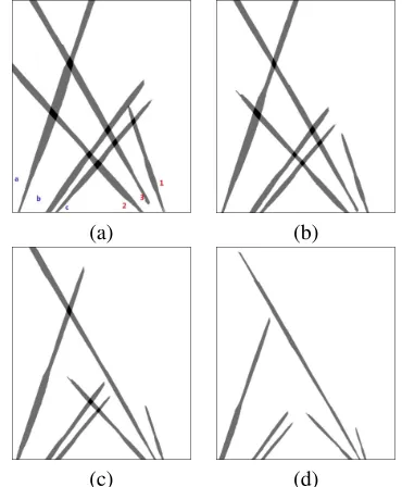
Fig. 5. Fusion of the projected foregrounds in the top view using homogra-phies for a set of parallel planes.

Fig.4 shows the procedure for the foreground detection us-ing background subtraction and GMM at frame 1200. Fig.4(a) and (b) are the original images. The results of foreground detection in the two camera views are shown in Fig.4(c) and (d). In each camera view, there are three pedestrians which are labelled with1to3 in camera viewaand labelled witha toc in camera viewb.

Each foreground polygon in a camera view was warped to the top view according to the homography for a set of planes. In these experiments, the 7 homography planes which are parallel to and 1.5-1.8 meter above the ground plane. These planes are around the head level of pedestrians. Fig.5 are foreground fusions using the homographies for the planes at heights of1.5m,1.6m,1.7m, and1.8m respectively.

Fig. 6. Intersection regions with homography at1.5mheight.

(a) (b)

Fig. 7. The warped back pixels overlaid on the foreground camera views.

in the top view is given the same label of the corresponding foreground region in individual camera views. The foreground projections intersect in 8 regions. Fig.6 shows the foreground intersection regions of homography mapping at 1.5m height. Each intersection region is given a label to indicate the corresponding foreground regions in the two camera views. For example, region1bis the intersection of foreground region 1 in camera viewa and foreground regionb in camera view b.

Then, each pixel in the intersection regions is warped back to each camera view according to the homographies for the ground plane and a plane at a height of 1.5 meters. In Fig.7, one pixel in the intersection region is warped back and overlaid on the individual foreground camera views. The blue dot and the red dot in each camera view indicate the warped back pixels according to the homographies for the ground plane and a plane at a height of 1.5 meters respectively. The yellow line in each camera view indicates all pixels on the line decided by the pair of warped back pixels in that view. The occupancy likelihood of original pixel in a single camera view is calculated.

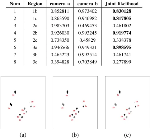
According to Eq.8, the occupancy map which indicates the likelihood that the intersection region is occupied by an real object is generated. Table I shows the result of the average value of occupancy likelihood for each intersection region. For intersection region1bin the top view, when each pixel in that region is warped back to camera view a, the average value of the occupancy likelihood in camera viewais 0.852811. Since the average value of the occupancy likelihood in camera viewb is 0.973402, the joint likelihood is 0.830128. The intersection regions which have the likelihood higher than 0.6 are in bold. To visualize the results, in Fig.8, each intersection region in the top view is filled with its average likelihood, in which the darkest intensity marks the highest likelihood.

Since colour matching is carried out in each camera view,

TABLE I

THE RESULT OF THE AVERAGE VALUE OF OCCUPANCY LIKELIHOOD FOR EACH INTERSECTION REGION.

Num Region camera a camera b Joint likelihood

1 1b 0.852811 0.973402 0.830128

2 1c 0.863590 0.946982 0.817805

3 2a 0.983703 0.469453 0.461802 4 2b 0.926030 0.993245 0.919774

5 2c 0.738350 0.45829 0.338378 6 3a 0.946566 0.949321 0.898595

7 3b 0.465223 0.992514 0.461741 8 3c 0.394828 0.703849 0.277899

(a) (b) (c)

Fig. 8. The visualized results of the occupancy likelihood map, (a) in camera viewa, (b) in camera viewb, and (c) joint likelihood map.

according to the inversed homography for the plane at a height of 1.5 meter, the intersection regions in the top view are warped back into the individual camera views to generate the warped back patches. Fig.9 are the warped back patches overlaid on the original camera views. The regions with blue boxes are the warped back patches. Each warped back patch is given the same label of the corresponding intersection region in the top view. Table II shows the colour matching results. The HSI color space is used in the color matching. Since the Mahalanobis distances of the unmatched intersection regions are usually much greater then 10000, the data in bold indicates the matched intersection regions. The intersection regions 2, 4 and6 in Table II are identified as the matched regions.

Table III shows the results using 7 planes. The intersections 2, 4 and 6 which has the highest height and its occupancy likelihood is higher than a threshold, color matching result is lower than a threshold, area is over a threshold indicate the location of person’s head top. Their corresponding heights are 1.5m,1.75and1.75.

(a) (b)

TABLE III

THE RESULT OF THE AVERAGE VALUE OF OCCUPANCY LIKELIHOOD FOR INTERSECTION REGIONS WITH MULTIPLE LAYERS.

Num Region 1.5 1.55 1.6 1.65 1.7 1.75 1.8 1.8

1 1b 0.830128 - - - phantom

2 1c 0.817805 0.781195 - - - 1.5

3 2a 0.461802 0.488151 0.524917 0.636869 - - - phantom 4 2b 0.919774 0.900628 0.904515 0.897847 0.887763 0.900970 - 1.75 5 2c 0.338378 0.449027 0.445362 0.486092 0.514107 0.573203 - phantom 6 3a 0.898595 0.995712 0.978885 0.955467 0.945971 0.964359 - 1.75 7 3b 0.461741 0.471828 0.498279 0.519372 - - - phantom 8 3c 0.277899 0.293784 0.332454 0.372789 - - - phantom

TABLE II

THE COLOUR MATCHING RESULTS.

Num Region Joint likelihood

1 1b 4178670

2 1c 615

3 2a 1125400

4 2b 2551

5 2c 33591

6 3a 2327

7 3b 187247

8 3c 693683

VII. CONCLUSION

A pedestrian detection approach using occupancy informa-tion and color cue with multiple homographies is proposed in this paper. The foreground regions detected in each camera view are warped into a set of virtual top views according to the homography for a planes at different height. The intersection regions in each top view indicate al the possible regions that contain real objects. To identify the false-positive detections, which occur due to the foreground intersections of non-corresponding objects in the top view, the occupancy information and colour matching are applied successively. For a set of intersection regions corresponding to the same foreground projection, the intersection region which has the highest height is recognized as the location of a person’s head top. This method can overcome the problems in single pixelwise color matching methods. Experiments have shown the robustness of this algorithm.

ACKNOWLEDGMENT

This work is supported by the National Natural Science Foundation of China (NSFC) under Grant 60975082.

REFERENCES

[1] Q. Cai and J. K. Aggarwal, “Automatic tracking of human motion in indoor scenes across multiple synchronized video streams,” inComputer Vision, 1998. Sixth International Conference on. IEEE, 1998, pp. 356– 362.

[2] O. Javed, S. Khan, Z. Rasheed, and M. Shah, “Camera handoff: tracking in multiple uncalibrated stationary cameras,” inHuman Motion, 2000. Proceedings. Workshop on. IEEE, 2000, pp. 113–118.

[3] V. Kettnaker and R. Zabih, “Bayesian multi-camera surveillance,” in Computer Vision and Pattern Recognition, 1999. IEEE Computer Society Conference on., vol. 2. IEEE, 1999.

[4] M. Quaritsch, M. Kreuzthaler, B. Rinner, H. Bischof, and B. Strobl, “Au-tonomous multicamera tracking on embedded smart cameras,”EURASIP Journal on Embedded Systems, vol. 2007, no. 1, pp. 35–35, 2007. [5] S. Khan and M. Shah, “Consistent labeling of tracked objects in multiple

cameras with overlapping fields of view,”Pattern Analysis and Machine Intelligence, IEEE Transactions on, vol. 25, no. 10, pp. 1355–1360, 2003.

[6] G. P. Stein, “Tracking from multiple view points: Self-calibration of space and time,” in Computer Vision and Pattern Recognition, 1999. IEEE Computer Society Conference on., vol. 1. IEEE, 1999. [7] M. Xu, J. Orwell, L. Lowey, and D. Thirde, “Architecture and algorithms

for tracking football players with multiple cameras,”IEE Proceedings-Vision, Image and Signal Processing, vol. 152, no. 2, pp. 232–241, 2005. [8] W. Du and J. Piater, “Multi-camera people tracking by collaborative particle filters and principal axis-based integration,” inComputer Vision– ACCV 2007. Springer, 2007, pp. 365–374.

[9] W. Hu, M. Hu, X. Zhou, T. Tan, J. Lou, and S. Maybank, “Principal axis-based correspondence between multiple cameras for people tracking,” Pattern Analysis and Machine Intelligence, IEEE Transactions on, vol. 28, no. 4, pp. 663–671, 2006.

[10] J. Black and T. Ellis, “Multi camera image tracking,”Image and Vision Computing, vol. 24, no. 11, pp. 1256–1267, 2006.

[11] S. M. Khan, P. Yan, and M. Shah, “A homographic framework for the fusion of multi-view silhouettes,” inComputer Vision, 2007. ICCV 2007. IEEE 11th International Conference on. IEEE, 2007, pp. 1–8. [12] A. Mittal and L. Davis, “Unified multi-camera detection and tracking

using region-matching,” in Multi-Object Tracking, 2001. Proceedings. 2001 IEEE Workshop on. IEEE, 2001, pp. 3–10.

[13] A. Mittal and L. S. Davis, “M2tracker: A multi-view approach to segmenting and tracking people in a cluttered scene,” International Journal of Computer Vision, vol. 51, no. 3, pp. 189–203, 2003. [14] J. Berclaz, F. Fleuret, E. Turetken, and P. Fua, “Multiple object tracking

using k-shortest paths optimization,” Pattern Analysis and Machine Intelligence, IEEE Transactions on, vol. 33, no. 9, pp. 1806–1819, 2011. [15] S. M. Khan and M. Shah, “Tracking multiple occluding people by localizing on multiple scene planes,” Pattern Analysis and Machine Intelligence, IEEE Transactions on, vol. 31, no. 3, pp. 505–519, 2009. [16] R. Eshel and Y. Moses, “Tracking in a dense crowd using multiple cameras,”International journal of computer vision, vol. 88, no. 1, pp. 129–143, 2010.

[17] A. Criminisi, I. Reid, and A. Zisserman, “Single view metrology,” International Journal of Computer Vision, vol. 40, no. 2, pp. 123–148, 2000.

[18] C. Stauffer and W. E. L. Grimson, “Adaptive background mixture models for real-time tracking,” in Computer Vision and Pattern Recognition, 1999. IEEE Computer Society Conference on., vol. 2. IEEE, 1999. [19] M. Xu, J. Ren, D. Chen, J. Smith, and G. Wang, “Real-time detection via

homography mapping of foreground polygons from multiple cameras,” inImage Processing (ICIP), 2011 18th IEEE International Conference on. IEEE, 2011, pp. 3593–3596.