Analysis of time-lapse travel-time and amplitude changes to assess reservoir compartmentalisation

This is a repository copy of

Analysis of time-lapse travel-time and amplitude changes to

assess reservoir compartmentalisation

.

White Rose Research Online URL for this paper:

http://eprints.whiterose.ac.uk/82323/

Version: Accepted Version

Article:

He, Y, Angus, DAC, Clark, RA et al. (1 more author) (2016) Analysis of time-lapse

travel-time and amplitude changes to assess reservoir compartmentalisation. Geophysical

Prospecting, 64 (1). pp. 54-67. ISSN 0016-8025

https://doi.org/10.1111/1365-2478.12250

eprints@whiterose.ac.uk https://eprints.whiterose.ac.uk/ Reuse

Unless indicated otherwise, fulltext items are protected by copyright with all rights reserved. The copyright exception in section 29 of the Copyright, Designs and Patents Act 1988 allows the making of a single copy solely for the purpose of non-commercial research or private study within the limits of fair dealing. The publisher or other rights-holder may allow further reproduction and re-use of this version - refer to the White Rose Research Online record for this item. Where records identify the publisher as the copyright holder, users can verify any specific terms of use on the publisher’s website.

Takedown

If you consider content in White Rose Research Online to be in breach of UK law, please notify us by

Analysis of time-lapse travel-time and amplitude changes to assess reservoir

compartmentalization

Y-X. He!, D.A. Angus, R.A. Clark and M.W. Hildyard

School of Earth & Environment, University of Leeds, Leeds, LS2 9JT, United Kingdom.

E-mail: eeyhe@leeds.ac.uk.

ABSTRACT

Fluid depletion within a compacting reservoir can lead to significant stress and strain changes and

potentially severe geomechanical issues, both inside and outside the reservoir. We extend previous

research of time-lapse seismic interpretation by incorporating synthetic near-offset and full-offset

common-midpoint reflection data using anisotropic ray tracing to investigate uncertainties in

time-lapse seismic observations. The time-time-lapse seismic simulations use dynamic elasticity models built

from hydro-geomechanical simulation output and a stress-dependent rock physics model. The

reservoir model is a conceptual two-fault graben reservoir, where we allow the fault fluid-flow

transmissibility to vary from high to low to simulate non-compartmentalized and compartmentalized

reservoirs respectively. The results indicate time-lapse seismic amplitude changes and traveltime shifts

can be used to qualitatively identify reservoir compartmentalization. Due to the high repeatability and

good quality of the time-lapse synthetic dataset, the estimated traveltime shifts and amplitude

changes for near-offset data match the true model subsurface changes with minimal errors. A 1D

velocity-strain relation was used to estimate the vertical velocity change for the reservoir bottom

interface by applying zero-offset time-shifts from both the near-offset and full-offset measurements.

For near-offset data, the estimated P-wave velocity changes were within 10% of the true value.

However, for full-offset data, time-lapse attributes are quantitatively reliable using standard time-lapse

seismic methods when an updated velocity model is used rather than the baseline model.

Key words: Time-lapse seismic estimates, Waveform modelling, Reservoir compartmentalization.

1 INTRODUCTION

Reservoir production can cause serious geomechanical issues in a reservoir and the surrounding rocks,

pressure inside a producing reservoir has been observed in a number of reservoirs in the Gulf of Mexico

and North Sea, particularly in the high-porosity, over-pressured (HPHT) sand and chalk reservoirs with

large thickness (e.g., Guilbot and Smith 2002; Hawkins et al. 2007; Herwanger and Horne 2009).

Reservoir compaction due to production can act as a major driving mechanism for fluid flow by

maintaining pressure. Due to reservoir heterogeneity and geometry, hydrocarbon production can lead to

reservoir compartmentalization and subsequent heterogeneous pore pressure distribution. Furthermore,

large strain and stress changes in the overburden might lead to wellbore failure due to shear or fault

reactivation and hence cause serious economic loss. Monitoring and understanding stress and reservoir

pressure changes across faults (or any barrier) is therefore of considerable significance to avert drilling

and reservoir depletion related problems.

Time-lapse seismic monitoring of production-induced changes in a reservoir and the surrounding rocks

over time has the basic aim of mapping reservoir compartments and subsurface rock deformation,

identifying by-passed oil, monitoring fluid movement and planning for future production performance (e.g.,

Calvert 2005; Herwanger and Koutsabeloulis 2011). The general idea behind the time-lapse seismic

approach is to enable separation of the effects of fluid saturation and pore pressure changes, and this

has been challenging (Landr¿ 2001; Trani et al. 2011; MacBeth et al. 2011). Since reservoir

compaction and pore pressure changes induced by fluid depletion in a reservoir might lead to

changes in seismic velocities and layer thickness, it is thus crucial to discriminate between the two

effects using time-lapse seismic analysis.

Using a 1D expression to describe the travel-time difference due to geomechanical effects (equation

1, Landr¿ and Stammeijer 2004), Hatchel and Bourne (2005) and R¿ste, Stovas and Landr¿ (2005)

propose a linearized relation to link changes in layer velocity and thickness using a dilation factor.

Using the dilation factor and assuming uniaxial deformation, vertical velocity change and average

vertical strain can be estimated from observed time-lapse vertical travel-time shifts. Moving beyond

uniaxial deformation, Minkoff et al. (2004) apply coupled fluid-flow and geomechanical simulations

capable of predicting production-induced triaxial (3D) stress evolution and deformation within a

compacting reservoir. Herwanger and Horne (2009) extend this workflow to predict induced seismic

anisotropy and velocity changes due to 3D stress and strain evolution within and outside a reservoir.

Bakulin 2004) to estimate seismic velocity perturbations caused by production induced effective

stress changes. Fuck, Bakulin and Tsvankin (2009) and Fuck, Tsvankin and Bakulin (2011) introduce

an analytic geomechanical model with third-order elasticity to predict travel-time shifts due to

stress-induced seismic velocity heterogeneity and anisotropy within and surrounding a compacting reservoir.

Verdon et al. (2008) and Angus et al. (2009) and Angus, Fisher and Verdon (2012) extend and

calibrate a micro-structural rock-physics approach to model the nonlinear elastic response due to

varying effective stress and hence predict induced changes in seismic velocity and anisotropy.

Verdon et al. (2011) and Angus et al. (2011) integrate the micro-crack rock physics model with coupled

fluid-flow and geomechanical simulation (Segura et al. 2011) for seismic modelling applications to

evaluate various time-lapse seismic and microseismic attributes. The primary reason for using the

micro-crack model rather than the third-order elasticity model is based on practical considerations;

most ultrasonic stress-dependent velocity measurements do not include the strain measurements

needed for third-order elasticity theory.

In spite of many successful applications of the time-lapse seismic technique for reservoir monitoring

(Barkved 2012) and hydro-geomechanical calibration (Herwanger et al. 2010), various uncertainties

exist. These uncertainties exist for several reasons, but primarily they relate to the fact that the

hydro-geomechanical and rock physics models are simplified representations of the true physics.

Furthermore, there is the question of how best to process time-lapse seismic data. Smith and

Tsvankin (2012) analyze the stress and strain-induced travel-time shifts using coupled fluid-flow and

geomechanical simulation, third-order elasticity rock physics model and multicomponent full-waveform

finite-difference seismic modeling. To the authorsÕ knowledge, Smith and Tsvankin (2012) provide the

first study using full waveform synthetic data to develop a processing workflow that includes f-k

(frequency-wavenumber) filtering of shot records, cross-correlation skip corrections and an adaptive

polynomial time-shift curve fitting. The integration of time-lapse seismic analysis and

hydro-geomechanical simulation can strengthen our understanding of the evolution of the dynamic reservoir

system, and hence lead to a better quantification of trapped oil, optimization of well placement and

design, and hydrocarbon extraction procedure.

In this paper we use ray-based waveform forward modelling to investigate the fidelity of time-lapse

be used to identify reservoir compartmentalization. The ray-based synthetics allow us to avoid

complications from multiple energy in the processing as well as provide fast synthetic waveforms for

3D generally anisotropic velocity models. The dynamic elastic models constructed from

hydro-geomechanical simulation and non-linear micro-crack rock physics models are considered the

ground-truth model. Estimated time-lapse seismic attributes (travel-time shifts and reflection

amplitude changes) are compared with the dynamic elastic models to study the effects of errors

resulting from time-lapse seismic processing and time-lapse seismic attribute calculations.

Understanding these errors is necessary for meaningful calibration of hydro-geomechanical models

and improving subsurface reservoir predictions. A major objective of this study is to develop a method

of being able to study, both qualitatively and quantitatively, the influences of these errors in time-lapse

seismic observations by using an integrated fluid-flow and geomechanical simulation, rock physics

model and seismic simulation.

2 METHODOLOGY

In time-lapse seismic studies, there are two approaches to reduce uncertainty in reservoir predictions

and enhance the imaging quality of by-passed reserves (Davies and Maver 2004): simulation to

seismic and seismic to simulation. In both approaches, the workflow requires the integration of

hydro-geomechanical simulation, rock physics models and time-lapse seismic analysis. To quantitatively

monitor and measure small subsurface physical changes, we need to understand the magnitude of

errors inherent in time-lapse seismic analysis and hence how much the true time-lapse changes might

be over-predicted or under-predicted due to these errors.

[FIGURE 1 HERE]

In this paper, we focus on developing the forward modelling (simulation to seismic) approach (see

Figure 1). Specifically, the dynamic elastic models at three stages of production (baseline survey,

5-year and 10-5-year monitor surveys) are used as the input elastic models for 3D seismic waveform

simulation. The waveform synthetics are processed using various methodologies and subsequently

compared directly with the dynamic elastic models to evaluate the errors in the conventional

time-lapse estimates, and hence potential errors and uncertainties in the time-time-lapse seismic observations

(He et al. 2013). In principle, deviations between the synthetics and the true time-lapse seismic

rock physics model, but it is expected that the major influence will be due to the band-limited nature of

seismic waveforms (i.e., resolution), acquisition geometry and time-lapse seismic processing.

2.1 Two-fault graben reservoir model

The subsurface model we use in this study is a graben-style reservoir consisting of three reservoir

compartments separated by two normal faults (Angus et al. 2010; Lynch et al. 2013). Two production

cases are examined, one having high fault fluid-flow transmissibility (HFT) and the other having low

fault fluid-flow transmissibility (LFT). Figure 2 shows the geometry of the model, with the production

well located in the centre of the left-most reservoir compartment. Hydro-geomechanical simulation is

performed using two-way iteratively coupled reservoir flow simulator Tempest with geomechanical

solver Elfen (Segura et al. 2011), where the geomechanical simulator uses pore pressure evolution

calculated in the reservoir simulator to update the geomechanical loading and the reservoir simulator

uses the updated pore volume change calculated in the geomechanical simulator to update the flow

properties. In the simulation, the production well is produced at a constant rate of 4000 m3/day at a

minimum well pressure of 5 MPa over the duration of the simulation. The stress, pressure and static

elastic tensor are output every six months of simulation time and are used as input for the non-linear

rock physics model of Verdon et al. (2008) to construct the dynamic elastic models for waveform

simulation (Angus et al. 2011).

[FIGURE 2 HERE]

Since the hydro-geomechanical mesh is unstructured, the dynamic elastic model is discretised on an

appropriate regular grid with arbitrary spatial density suitable for ray tracing via a B-spline

interpolation algorithm. As well, since ray tracing requires a smooth velocity model, the elastic model

is also smoothed using a damped least squares method to remove sharp interfaces as well as sharp

transitions in elastic properties. Figure 3 shows an example of the 3D P-wave velocity model after

interpolation and smoothing. Also shown in Figure 3 is a 1D P-wave velocity profile through the centre

of the left reservoir-compartment that compares the original, interpolated and smoothed velocities.

[FIGURE 3 HERE]

Given the asymmetry and heterogeneity of the graben model, stress perturbations will be triaxial and

influence of induced seismic anisotropy as well as induced velocity heterogeneity on estimated

time-lapse seismic attributes (e.g., Hawkins et al. 2007; Herwanger and Horne 2009), both anisotropic

elastic models and equivalent isotropic elastic models are constructed. The isotropic model assumes

vertical effective stress changes only, and hence the elastic tensor C33 is used to compute the P-wave

velocity.

2.2 Acquisition geometry and waveform synthetics

An anisotropic ray tracer (Guest and Kendall 1993) is used to generate seismic synthetics. The

simulation uses both ray shooting (variable incidence and azimuth angles) and normal incidence (e.g.,

exploding reflector method) modes. Figure 4 shows an example of the ray shooting method for one

shot with various incidence angles and tracking two reflectors; in this paper we focus on the top and

bottom reservoir layers (two red interfaces) to examine the time-lapse seismic responses due to

triaxial effective stress changes and strain within and outside the reservoir. P-wave explosive point

sources were simulated using a zero-phase Ricker wavelet with central frequency of 30 Hz and

temporal sample of 1 ms, positioned along the surface and down the centre of the long-axis

(x-direction) of the model. The source-receiver offsets vary from 0 m to 5500 m, with receiver spatial

spacing of 12.5 m.

[FIGURE 4 HERE]

The synthetic shot gather data are resorted into common-mid point (CMP) gathers, normal-moveout

(NMO) corrected, stacked and time-migrated using the Stolt migration method. Figure 5 shows a

post-stack migrated image of baseline model using the reflections from the two reservoir layers. Identical

acquisition geometry, source wavelet and processing procedures were applied to the baseline, 5-year

monitor (monitor1) and 10-year monitor (monitor2) surveys such that time-lapse seismic repeatability

is not an issue with the subsequent analysis. Although it is expected that the post-stack near-offset

data will provide better vertical resolution of time-lapse seismic changes than post-stack full-offset

data (due to offset effects), the post-stack full-offset data should contain more information on induced

lateral velocity heterogeneity within the subsurface. Since near-offset data contains mainly

sub-vertically propagating energy, the information carried by near-offset reflections will be dominated by

vertical velocity variation. Full-offset data contain sub-vertical as well as oblique incident reflections

near- and full-offset time-lapse reflection seismic analysis with the true dynamic elastic model for both

isotropic and anisotropic medium, we use vertical incidence synthetics (utilizing the normal incidence

ray tracing) to provide the benchmark travel-time shifts and reflection amplitude changes.

[FIGURE 5 HERE]

2.3 Calculation of time-lapse seismic attributes

The standard time-lapse seismic attribute, travel-time shift, is calculated by cross-correlation of the

baseline and monitor surveys. We use a Hanning window with length of 80 ms and 66 ms for the top

and bottom reservoir horizons (such that the window length encompasses the reflection events that

have approximate period of 70 ms and 50 ms for the top and bottom horizons respectively). The

time-shift is calculated by interpolating the time lag for maximum cross-correlation (i.e., to improve the

resolution of estimated travel-time shifts). The reflection amplitude changes are estimated first by

correcting for the travel-time shift between traces and then calculating the difference between the

maximum reflection amplitudes of both traces (see Figure 6). Previous studies (e.g., Hodgson 2009;

Selwood 2010; Whitcombe et al. 2010) have shown that the conventional cross-correlation technique

is not ideal for time-lapse seismic travel-time shift analysis. This is because travel-time shift recovery

using cross-correlation is dependent on window length (Selwood 2010), which could lead to

high-frequency noisy or incorrect estimates (Whitcombe et al. 2010). However, in this study we are

primarily concerned with the general recovery of time-lapse seismic attributes and so do not apply

more advanced methods of estimating time shifts.

[FIGURE 6 HERE]

3 Results: time-lapse seismic attributes

The reflection amplitudes estimated from the baseline, monitor1 and monitor2 surveys for both

isotropic and anisotropic HFT models are displayed in Figure 7. The amplitudes are normalised to the

largest magnitude of the baseline anisotropic model (in this case the largest amplitudes are for the left

and right top reservoir interface). The difference in amplitude change estimates between near-offset

data and the ground-truth is less than 10%. However, the difference in amplitude change estimates

using the full-offset data shows significantly larger deviations ranging between 20% and 50%,

The reflection coefficients along the reservoir interfaces are influenced by fluid depletion induced pore

pressure changes (we do not model saturation effects so that we can focus solely on pressure

effects). The absolute amplitude decrease indicates a velocity increase in the reservoir and decrease

in the surrounding overburden and under-burden (i.e., reservoir velocities approach that of the

surrounding rock). There is little difference in the magnitude of amplitude changes in the isotropic and

the anisotropic models (see Figure 7), and this suggests that induced velocity heterogeneity is more

dominant than induced seismic anisotropy. The amplitude changes in the central compartment are

significantly less than the left and right compartments (i.e., nearly 10%) as a result of stress arching

due to compaction and reservoir geometry (Angus et al. 2010). This indicates the importance of

recognising stress arching in the time-lapse signature. Assuming uniaxial deformation one might

incorrectly assume the central compartment is not as productive compared to the left and right

compartments.

[FIGURE 7 HERE]

In Figure 8, the reflection amplitudes calculated from the anisotropic LFT model for monitor1 and

monitor2 are displayed. Similar to the HFT model, the reflection amplitudes decrease for both the top

and bottom reservoir interfaces, though only in the left compartment (in the right and central

compartments the amplitude changes are negligible). This is because the low fluid-flow

transmissibility of both faults inhibits fluid flow from the central and right compartments to the

production well in the left compartment and hence pore pressure reduction is restricted to the left

compartment. The slight observable changes that occur in the central and right compartments relate

to stress arching due to stress redistribution in the overburden above the left compartment and fault

movement (Angus et al. 2010).

[FIGURE 8 HERE]

In Figure 9, the vertical travel-time shifts calculated from the near-offset and full-offset data for the

isotropic and anisotropic HFT models are displayed with the ground-truth model. The full-offset

travel-time shifts are larger than the near-offset travel-time shifts for both the top and bottom reservoir interfaces

(see Figure 9). In monitor1, the travel-time shift estimates are positive for the top interface and

negative for the bottom interface. For longer production and hence greater pore pressure reduction in

(-2 ms) to positive (5 ms). The increase in travel-time from the top interface results from reduced

velocity due to overburden extension. The initial decrease in travel-time from the bottom interface

results from increased velocity and layer compaction within the reservoir, and the transition to positive

shift is due to the evolving stress arching in the overburden.

[FIGURE 9 HERE]

Figure 10 demonstrates the time-lapse seismic travel-time shifts for the anisotropic LFT model. Larger

travel-time shift estimates for the full-offset data can be observed compared to the near-offset data

(similar to the results shown in Figure 9). The travel-time shifts are limited mainly to the left

compartment, though there are small negative travel-time shifts (-1 to -2 ms) over the central and right

compartments due to stress arching and reservoir geometry. In monitor2, the development of stress

arching in the overburden and side-burden has a significantly larger influence and leads to positive

travel-time shifts for the bottom layer.

[FIGURE 10 HERE]

The results from the time-lapse seismic attributes can be summarised as follows:

¥ The amplitude changes are sensitive to reservoir compaction relatively immediately, not only

locally close to the production well but also further away in the other compartments (for the

HFT model),

¥ The time shifts are less sensitive than the amplitude changes to reservoir compaction since

amplitude change is a more local attribute whereas time shift is a path-averaged attribute.

Since the time shift is a path-averaged attribute, it is effectively smoothed spatially and hence

the effect of time shifts away from the producing well can appear delayed temporally. This is

the main reason that the time strain attribute is used if the data are not too noisy, since the

time strain provides a localised measure of elastic property changes.

¥ Both amplitude changes and time shifts are sensitive to reservoir compartmentalization, and

¥ The influence of stress arching has a significant impact on the character of amplitude

A key observation is that post-stack near-offset seismic data provide a more accurate estimate of

time-lapse seismic attributes compared to post-stack full-offset data for conventional 4D seismic

processing (i.e., processing workflow that assumes uniaxial deformation). This has more to do with

the 4D seismic processing rather than the information contained in mid- and far-offset data. It is clear

that pre-stack time-lapse seismic analysis is more appropriate when the subsurface geometry and

induced velocity changes show strong lateral heterogeneity and anisotropy.

4 Estimating velocity change using 1D transform

The challenge in time-lapse seismic analysis is to find a suitable approach to discriminate between

velocity changes and induced strain, and hence quantitatively differentiate between the influence of

fluid saturation, where there is no strain, and reservoir pressure changes. Since travel-time shifts

represent the cumulative travel-time differences along the ray path, the seismic travel-time shift

attribute will not be a local measure of physical perturbations in the way that reflection amplitudes are.

However, the so-called time strain attribute provides an instantaneous (or interval) travel-time

difference measurement (Rickett et al. 2006) and can be calculated by taking the temporal derivative

of time shifts (

Δ

t

/

t

shift change for a single layer to describe the combined effects of fractional changes in layer

thickness and seismic velocity for normal incidence. Assuming

Δ

V

/

V

_<<

1

Δ

_z

/

_z

<<

1

and Stammeijer (2004) write

Δ

t

t

≈

Δ

z

z

−

Δ

V

V

=

ε

−

Δ

V

V

where

t

velocity and

zz

z

z

=

ε

Δ

/

Hatchell and Bourne (2005) and R¿ste et al. (2005) introduce a 1D linear model to link vertical strain

and velocity changes:

Δ

V

V

=

−

where the dimensionless factor

_R

_≥

0

0

≤

α

_R

α

time shifts from vertical velocity change and layer thickness change. Although this parameter cannot

provide an exact or unique relation between

Δ

V

/

V

ε

time-lapse seismic programs.

Hatchell and Bourne (2005) utilize a standard rock velocity-porosity relation with a theoretical crack

model to predict values for the dimensionless R-factor. The R-factor takes on two different values

depending on whether the layer is the reservoir unit or the overburden, and this is due to the

asymmetrical influence of rock compaction and elongation. Since the velocity-strain factor is assumed

to vary over a narrow range (typically between 2 and 3 for the reservoir, and between 4 and 6 in the

overburden layers), it has been applied with varying degrees of success on many fields. Herwanger

(2008) presents a method to compute the R-factor directly using third-order elasticity theory and

neglecting horizontal strain changes, yet notes that horizontal stress and strain have a significant

effect on vertical velocity changes. The dilator factor

α

properties and can vary spatially. R¿ste, Landr¿ and Hatchell (2007) introduce an approach to

calculate

α

within a given layer, and extend it to handle both lateral and vertical changes in thickness and

velocity.

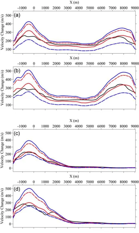
[FIGURE 11 HERE]

The estimated vertical P-wave velocity changes using the 1D velocity-strain model of Hatchell and

Bourne (2005) and the time strain attribute for the bottom reservoir interface of the HFT and LFT

models are shown in Figure 11. We compare velocity change estimates using the near-offset

travel-time shifts for four constant R-factors: (1) R=0 representative of no reservoir compaction or zero strain

(solid blue line), (2) R=1 for a value smaller than typically used for reservoirs and where velocity and

strain changes have equal influence on travel-time shifts (dashed blue line), (3) R=3 representative of

a value typically applied for reservoirs (solid red line), and (4) R=13 for a value larger than typically

used for reservoirs and where the time shift contribution is much larger for velocity change with

Comparing the estimated P-wave velocity changes with the true subsurface model it can be seen that

the constant non-zero R-factor cases provide a much more reliable estimate of velocity change (e.g.,

±20% error for R=3 compared to ±80% error for R=0) for both the HFT and LFT models. For the HFT

model, the estimated P-wave velocity changes for the constant non-zero R-value approaches that of

the true model in the central compartment with some deviations in the left and right compartments,

while the velocities estimated using zero strain R-value display large deviations (between ±30% to

±80% error) throughout the reservoir. This is consistent with the fact that compaction in the reservoir

is not homogeneous due to reservoir geometry and stress arching, and provides strong support for

allowing lateral variation in the dilation parameter (R¿ste et al. 2007). The estimated P-wave velocity

changes in monitor1 for the LFT model match well with the true model for the constant non-zero R

-values (within ±10% error). However, the velocity predictions worsen (±50% error) due to

production-related stress and strain heterogeneity after a longer period of production. The chosen constant R

-values used in the HFT models are larger than in the LFT models in order to yield similar velocity

predictions to the true model (the low fault transmissibility cases are approximately 50% the high

transmissibility cases). The different R-values relate to the varying amount of stress arching in the

overburden as well as magnitude of stress changes and strains in the reservoir.

Although the constant R-value approach yields vertical P-wave velocity change estimates with broad

similarity to the true subsurface model, the differences between the estimated and the true subsurface

models can still lead to serious errors when predicting fluid properties and stress changes to calibrate

hydro-geomechanical models. Error in velocity change estimates will propagate into errors in

estimating fluid saturation and pressure changes (Landr¿ 2001; Ribeiro and MacBeth 2004; Kvam

and Landr¿ 2005; Sayers 2006). When reservoir complexity and/or stress arching is expected to be

significant, a more accurate calculation of the velocity-strain relation (

_R

α

improve the time-lapse seismic velocity estimates. In the above example, we consider only vertical

strain and assume velocity changes have been modelled adequately using the 1D rock physics

model. However, induced seismic anisotropy and velocity heterogeneity due to triaxial strain and

stress changes within and outside the reservoir indicates that the approach of R¿ste, Stovas and

Landr¿ (2006) is likely a more appropriate method to estimate a ÔlaterallyÕ variable velocity-strain

5 Influence of velocity model on time-lapse seismic uncertainty

In conventional time-lapse seismic processing, both the baseline and monitor observations are

processed using identical workflows and, in many instances, the same velocity model (i.e., baseline

model), as discussed in Landr¿ and Stammeijer (2004). When the subsurface velocity changes are

small or only the near-offset data are used, the estimated time-lapse seismic travel-time shifts will be

quantitatively close to the true model values (e.g., fractional ms error as shown in Figures 9 and 10).

However, if the time-lapse velocity changes are significant, accurate velocity analysis for the monitor

surveys should be implemented to improve travel-time shift predictions and reduce artificial time-lapse

error and uncertainty in the time-lapse seismic attributes. In Figure 12, travel-time shift calculations

using the baseline and monitor P-wave velocity models in the stacking and Stolt time-migration

procedure are compared. Apparent improvements in the travel-time shifts for the full-offset data using

the monitor velocity model are observed and, as expected, very little improvement in the near-offset

data. This is because the travel times of full-offset stacks strongly depend on the lateral heterogeneity

and non-hyperbolic move-out. Thus, using post-stack full-offset data for time-lapse seismic attribute

analysis requires an accurate monitor velocity model when large velocity changes are expected. This

is because large velocity changes can cause noticeable time-lapse lateral and vertical shifts through

the migrated image (Cox and Hatchell 2008). However, accurate velocity analysis may be either

expensive or impractical for time-lapse surveys, and hence the uncertainty in velocity analysis should

be incorporated in time-lapse seismic analysis (see Kvam and Landr¿ 2005).

[FIGURE 12 HERE]

6 CONCLUSIONS

In this study, integrated hydro-geomechanical simulation, rock physics model and waveform seismic

simulation is applied to investigate the effects of time-lapse subsurface changes on P-wave attributes.

The workflow is applied on a two-fault graben reservoir model with time-variant rock properties due to

reservoir production induced effective stress changes inside and outside a reservoir. Travel-time

shifts and reflection amplitude changes are used to evaluate physical changes within the reservoir

system. The application of time-lapse seismic analysis was helpful to assess reservoir

compartmentalization from a qualitative and semi-quantitative estimate. The results indicate that

reservoir if quantitatively accurate estimates are required. Near-offset and full-offset synthetic

datasets of high repeatability and quality for baseline and repeated surveys were used to interpret the

time-lapse anomalies. The calculated time-lapse P-wave velocities were in general agreement with

the true subsurface models when using a constant R-value (for both the high and low fault fluid-flow

transmissibility models) in the reservoir. Differences in velocity predictions indicate that the producing

reservoir is not experiencing uniaxial deformation and that compaction and velocity changes are

variable laterally and hence require variable velocity-strain coefficients.

ACKNOWLEDGEMENTS

We would like to thank the associate editor and the two anonymous reviewers for helpful comments to

improve the paper. We are grateful to Centre of Integrated Petroleum Engineering and Geoscience,

University of Leeds for supporting this work. Y-X. He is supported by a China Scholarship

Council/University of Leeds scholarship and D.A. Angus is partially supported by a Research Councils

UK Fellowship. We thank Rockfield Software for access to the geomechanical simulator ELFEN, and

Roxar for access to the geological model builder RMS (TEMPEST).

REFERENCES

Angus D.A., Fisher Q.J. and Verdon J.P. 2012. Exploring trends in microcrack properties of sedimentary rocks: An audit of dry and water saturated sandstone core velocity-stress

measurements. International Journal of Geosciences3, 822-833.

Angus D.A., Kendall J.M., Fisher Q.J., Segura J.M., Skachkov S., Crook A.J.L. and Dutko M.

2010. Modelling microseismicity of a producing reservoir from coupled fluid-flow and geomechanical

simulation. Geophysical Prospecting58, 901-914.

Angus D.A., Verdon J.P., Fisher Q.J. and Kendall J.M. 2009. Exploring trends in microcrack properties of

sedimentary rocks: an audit of dry-core velocity-stress measurements. Geophysics74, E193-E203. Angus D.A., Verdon J.P., Fisher Q.J., Kendall J-M., Segura J.M., Kristiansen T.G., Crook A.J.L.,

Skachkov S., Yu J. and Dutko M. 2011. Integrated fluid-flow, geomechanic and seismic modeling for

reservoir characterisation. Canadian Society of Exploration Geophysicists Recorder36, 26-35. Barkved O.I. 2012. Seismic Surveillance for Reservoir Delivery. EAGE Publications.

Calvert R. 2005. Insights and Methods for 4D Reservoir Monitoring and Characterization. EAGE

Publications.

Cox B. and Hatchell P. 2008. Straightening out lateral shifts in time-lapse seismic. First Break26, 93-98. Davies D. and Maver K.G. 2004. 4D Time-Lapse Studies and Reservoir Simulation to Seismic Modelling.

Offshore Technology Conference, Houston, USA, Expanded Abstracts, 16934.

Fuck R.F., Bakulin A. and Tsvankin I. 2009. Theory of traveltime shifts around compacting reservoirs: 3D

solutions for heterogeneous anisotropic media. Geophysics74, D25-D36.

compacting reservoirs. Geophysical Prospecting59, 78-89. Guest W.S. and Kendall J.M. 1993. Modeling seismic waveforms in anisotropic inhomogeneous media

using ray and Maslov asymptotic theory: application to exploration seismology. Canadian Journal of

Exploration Geophysics29, 78-92.

Guilbot J. and Smith B. 2002. 4D constrained depth conversion for reservoir compaction estimation:

Application to Ekofisk Field. The Leading Edge21, 302-308.

Hatchell P.J. and Bourne S.J. 2005. Measuring reservoir compaction using time-lapse time shifts. 75th

SEG meeting, Houston, USA, Expanded Abstracts, 2500-2503.

Hawkins K., Howe S., Hollingworth S., Conroy G., Ben-Brahim L., Tindle C., Taylor N., Joffroy G.

and Onaisi A. 2007. Production-induced stresses from time-lapse time shifts: A geomechanics case

study from Franklin and Elgin fields, The Leading Edge26, 655-662.

He Y-X., Angus D.A., Hildyard M.W. and Clark R.A. 2013. Time-lapse seismic waveform modeling:

Anisotropic ray tracing using hydro-mechanical simulation models. 75th EAGE meeting, London, U.K.,

Expanded Abstracts, We-12-16.

Herwanger J.V. 2008. R we there yet? 70th EAGE meeting, Rome, Italy, Expanded Abstracts, I029.

Herwanger J.V. and Horne S.A. 2009. Linking reservoir geomechanics and time-lapse seismic: Predicting

anisotropic velocity changes and seismic attributes. Geophysics74, W13-W33.

Herwanger J.V. and Koutsabeloulis N. 2011. Seismic Geomechanics: How to Build and Calibrate

Geomechanical Models using 3D and 4D Seismic Data. EAGE Publications.

Herwanger J.V., Schi¿tt C.R., Frederiksen R., If F., Vejbᴂ_{k O.V., Wold R., Hansen H.J., Palmer E. and}

Koutsabeloulis N. 2010. Applying time-lapse seismic methods to reservoir management and field

development planning at South Arne, Danish North Sea. Petroleum Geology Conference series, 7, 523-535.

Hodgson N. 2009. Inversion for reservoir pressure change using overburden strain measurements

determined from 4D seismic. PhD Dissertation, Heriot-Watt University.

Kvam ¯. and Landr¿ M. 2005. Pore-pressure detection sensitivities tested with time-lapse seismic data.

Geophysics70, O39-O50.

Landr¿ M. 2001. Discrimination between pressure and fluid saturation change from time-lapse seismic

data. Geophysics66, 836-844.

Landr¿ M. and Stammeijer J. 2004. Quantitative estimation of compaction and velocity changes using 4D

impedance and traveltime changes. Geophysics 69, 949-957.

Lynch T., Angus D., Fisher Q. and Lorinczi P. 2013. The impact of geomechanics on monitoring

techniques for CO2 injection and storage. Energy Procedia37, 4136-4144.

MacBeth C., HajNasser Y., Stephen K. and Gardner A. 2011. Exploring the effect of meso-scale shale

beds on a reservoirÕs overall stress sensitivity to seismic waves. Geophysical Prospecting59, 90-110. Minkoff S.E., Stone C.M., Bryant S. and Peszynska M. 2004. Coupled geomechanics and flow simulation

for time-lapse seismic modelling. Geophysics69, 200-211.

Prioul R., Bakulin A. and Bakulin V. 2004. Nonlinear rock physics model for estimation of 3D subsurface

stress in anisotropic formations: Theory and laboratory verification. Geophysics69, 415-425.

using 4D seismic. 66th EAGE meeting, Paris, France, Expanded Abstracted, A042.

Rickett J., Duranti L, Hudson T. and Hodgson N. 2006. Compaction and 4-D time strain at the Genesis

Field. 76th SEG meeting, New Orleans, US, Expanded Abstract, 3215-3219.

R¿ste T., Landr¿ M. and Hatchell P. 2007. Monitoring overburden layer changes and fault movements

from time-lapse seismic data on the Valhall field. Geophysical Journal International170, 1100-1118. R¿ste T., Stovas A. and Landr¿ M. 2005. Estimation of layer thickness and velocity changes using 4D

prestack seismic data. 67th EAGE meeting, Madrid, Spain, Expanded Abstracts, C010.

R¿ste T., Stovas A. and Landr¿ M. 2006. Estimation of layer thickness and velocity changes using 4D

prestack seismic data. Geophysics71, S219-S234.

Sayers C. 2006. An introduction to velocity-based pore-pressure estimation. The Leading Edge25, 1496-1500.

Segura J.M., Fisher Q.J., Crook A.J.L., Dutko M., Yu J.G., Skachkov S., Angus D.A., Verdon J.P. and

Kendall J-M. 2011. Reservoir stress path characterization and its implications for fluid-flow production

simulations. Petroleum Geoscience17, 335-344.

Selwood C. 2010. Researching the optimum bandwidth to extract 4D time shifts. M.Sc. Dissertation,

University of Leeds.

Smith S.S. and Tsvankin I. 2012. Modeling and analysis of compaction-induced traveltime shifts for

multicomponent seismic data. Geophysics77, T221-T237.

Trani M., Arts R., Leeuwenburgh O., and Brouwer J. 2011. Estimation of changes in saturation and

pressure from 4D seismic AVO and time-shift analysis. Geophysics76, C1-C17.

Verdon J.P., Angus D.A., Kendall J-M. and Hall S.A. 2008. The effect of microstructure and nonlinear

stress on anisotropic seismic velocities. Geophysics73, D41-D51.

Verdon J.P., Kendall J-M., White D.J. and Angus D.A. 2011. Linking microseismic event observations

with geomechanical models to minimise the risks of storing CO2 in geological formations. Earth and

Planetary Science Letters305, 143-152.

Whitcombe D.N., Paramo P., Philip N., Toomey A., Redshaw T. and Linn S. 2010. The correlated

leakage method Ð itÕs application to better quality timing shifts on 4D data. 72nd EAGE meeting,

FIGURES: