This is a repository copy of
Fitting the two-compartment model in DCE-MRI by linear
inversion
.
White Rose Research Online URL for this paper:
http://eprints.whiterose.ac.uk/89652/
Version: Accepted Version
Article:
Flouri, D, Lesnic, D and Sourbron, S (2016) Fitting the two-compartment model in
DCE-MRI by linear inversion. Magnetic Resonance in Medicine, 76 (3). pp. 998-1006.
ISSN 0740-3194
https://doi.org/10.1002/mrm.25991
Reuse
Unless indicated otherwise, fulltext items are protected by copyright with all rights reserved. The copyright exception in section 29 of the Copyright, Designs and Patents Act 1988 allows the making of a single copy solely for the purpose of non-commercial research or private study within the limits of fair dealing. The publisher or other rights-holder may allow further reproduction and re-use of this version - refer to the White Rose Research Online record for this item. Where records identify the publisher as the copyright holder, users can verify any specific terms of use on the publisher’s website.
Takedown
If you consider content in White Rose Research Online to be in breach of UK law, please notify us by
Fitting the two-compartment
model in DCE-MRI by linear
inversion
Dimitra Flouri1,2, Daniel Lesnic2 and Steven Sourbron1
Division of Biomedical Imaging1 and Department of Applied
Mathematics2, University of Leeds, Leeds LS2 9JT, UK
Accepted by Magnetic Resonance in Medicine
Abstract
Purpose
Model fitting of DCE-MRI data with non-linear least squares (NLLS) methods is slow and may be biased by the choice of initial values. The aim of this study was to develop and evaluate a linear least-squares (LLS) method to fit the two-compartment exchange and -filtration mod-els.
Methods
A second-order linear differential equation for the mea-sured concentrations was derived where model parameters act as coefficients. Simulations of normal and pathological data were performed to determine calculation time, accu-racy and precision under different noise levels and tempo-ral resolutions. Performance of the LLS was evaluated by comparison against the NLLS.
Results
The LLS method is about 200 times faster, which reduces the calculation times for a 256×256 MR slice from 9 min to 3 sec. For ideal data with low noise and high temporal resolution the LLS and NLLS were equally accurate and precise. The LLS was more accurate and precise than the NLLS at low temporal resolution, but less accurate at high noise levels.
Conclusion
The data show that the LLS leads to a significant
reduc-tion in calculareduc-tion times, and more reliable results at low noise levels. At higher noise levels the LLS becomes ex-ceedingly inaccurate compared to the NLLS, but this may be improved by using a suitable weighting strategy.
INTRODUCTION
Dynamic contrast-enhanced magnetic resonance imaging MRI (DCE-MRI) involves the serial acquisition of T1-weighted MR images before, during, and after an intra-venous administration of contrast agent. Tracer-kinetic analysis of the data produces physiological parameters such as tissue blood flow, capillary permeability, and the volume of the extravascular, extracellular space (1).
The most common class of tracer-kinetic models are the multi-compartment models, which are also widely used in other modalities such as positron-emission tomography (PET) and computed tomography (CT). Current stan-dards in DCE-MRI are the two- or three parameter Patlak and Tofts models (2, 3), which do not produce a measure-ment of tissue blood flow. In recent years, the increasing availability of DCE-MRI at high temporal resolution has promoted the use of four-parameter flow-weighted models such as the two-compartment exchange model (2CXM) (4) and the renal two-compartment filtration model (2CFM) (5, 6).
Non-linear least squares (NLLS) methods are the most commonly used algorithms to fit the model to the data (7). They require a choice of initial values which is updated it-eratively using gradient-descent type methods, until the difference between predicted and measured data is mini-mal. The process is slow, and there is a risk of convergence to local minima (8, 9). If this happens the result is biased by the initial values. A potential solution is to repeat the fit over a grid of initial values, but this requires massive computing capacity for pixel-based analysis (10).
method for the extended Tofts model. Simulations demon-strated that this improves calculation times significantly without an associated cost in accuracy and precision. The method is rapidly becoming a standard in applications of DCE-MRI (12–15).
A LLS method for the more general 2CXM and 2CFM has not yet been proposed in the field of DCE-MRI, but in nuclear medicine it is well-known that such more gen-eral models can be linearised too (9, 16–20). The purpose of this study is to develop a LLS method for the 2CXM and 2CFM, and evaluate calculation time, accuracy and precision using simulated data. A standard NLLS with a single set of initial values is used as a point of comparison.
METHODS
Theory
Definitions
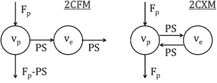
[image:3.612.55.268.488.570.2]The 2CXM and 2CFM are depicted graphically in Fig-ure 1. The key difference is that the flux out of the ex-travascular space is either directed back into the plasma space (2CXM) or directly to the outside (2CFM). Since the physiological interpretation of the parameters is not relevant for the purposes of the paper, the conventional notations of the 2CFM parameters (6) are modified to emphasize the symmetries and eliminate redundant nota-tions.
Figure 1: Diagrams of the 2CFM (left) and 2CXM (right).
The four independent model parameters are the plasma volume vp, the extravascular volume ve, the plasma flow
Fp and the permeability-surface area product P S. The
mean transit times of the blood (Tp), extravascular
com-partment (Te) and combined system (T) have the same
form in both models:
Tp= vp
Fp
, Te= ve
P S, T =
vp+ve
Fp
[1]
The measured tissue concentrationC(t) is a weighted av-erage of the concentrationscp(t) andce(t) in the individual
spaces:
C=vpcp+vece [2]
The mass-balance for ce(t) is the same for both models
(writingc′
efor the time-derivative of ce):
vec′e=P S(cp−ce) [3]
The difference between 2CXM and 2CFM lies in the mass-balance for cp(t). Given the arterial concentration ca(t),
we have (4, 6):
2CFM : vpc′p =Fp(ca−cp) [4]
2CXM : vpc′p =Fp(ca−cp) +P S(ce−cp) [5]
We assume thatcp(0) =ce(0) =ca(0) = 0 which
imme-diately leads to the initial conditions
C(0) =C′
(0) = 0 [6]
Non-Linear Least Squares
The NLLS method is based on an explicit analytical solu-tion of the models (⊗is convolution):
C(t) =Fp
T−T− T+−T−
e−t/T++ T+−T
T+−T− e−t/T−
⊗ca(t)
[7] The difference between 2CXM and 2CFM lies in the rela-tion betweenT± and the physiological parametersFp,vp,
P S, ve. The formulae are most straightforward in terms
of the mean transit times (Eqs.[1]):
2CFM : T+=Te, T−=Tp [8]
2CXM : T±=
1 2
T+Te± q
(T+Te)2−4TpTe
[9]
Linear Least Squares
The LLS method is based on a reduction of the two first-order differential equations for the unmeasurable con-centrations cp(t) and ce(t) (Eqs.[3, 4, 5]) to a single
second-order differential equation for the measurable con-centration C(t) (Eq.[2]). The derivation follows a stan-dard recipe that applies more generally to arbitrary N -compartment models (17).
We will present the derivation in more detail for the 2CFM alone, as the procedure is exactly the same for the 2CXM. First, differentiate Eq.[2] and use Eqs.[3, 4] to eliminatec′
e andc
′
p:
C′
=Fp(ca−cp) +P S(cp−ce) [10]
Then repeat the same process: differentiate Eq.[10], use Eqs.[3, 4] to eliminatec′
eandc′p, and simplify the result:
C′′
=Fpc′a−(Fp−P S)
Fp
vp
(ca−cp)−P S
P S ve
(cp−ce) [11]
We have now produced 3 equations (Eqs.[2,10,11]) that only contain two unknown functionscp(t) andce(t). The
first two of these equations are used to solve for these unknown functions, and the results are then inserted into the third. Explicitly, solving Eqs.[2,10] forcp andceleads
to:
cp=
P S C−(Fpca−C′)ve
P Svp+ (P S−Fp)ve
[12]
ce=
Fpvpca+ (P S−Fp)C−vpC′
P Svp+ (P S−Fp)ve
[13]
Inserting Eqs.[12, 13] into Eq.[11] then leads to a single second-order equation that only depends on the data C,
ca, and the unknown model parameters. The result is most
transparent when expressed in terms of the parametersFp,
T,Tp, Te. After some simplification a very similar result
arises for 2CFM and 2CXM:
C′′=−αC−βC′+γca+Fpc′a [14]
The parameters (α, β, γ) are defined as:
2CFM : α= 1
TeTp
, β= Te+Tp
TeTp
, γ= FpT
TeTp
[15]
2CXM : α= 1
TeTp
, β =Te+T
TeTp
, γ= FpT
TeTp
[16]
To avoid the problems associated with numerical differen-tiation of noisy data, Eq.[14] can be integrated twice over time. Using the following notation for the integral:
¯
f(t) =
Z t
0
f(τ)dτ [17]
this leads to:
C(t) =−αC¯¯(t)−βC¯(t) +γc¯¯a(t) +Fpc¯a(t) [18]
If the dataC(t) andca(t) are measured at N time points
t0, t1, . . . , tN−1, then Eq.[18] leads to a system ofN linear
equations. They can be summarised as a matrix equation
C = AX where C = [C(t0), . . . , C(tN−1)] is an array
holding the measured concentrations, andX= [α, β, γ, Fp]
contains the unknowns. The 4×N-element matrix Ais given explicitly by:
A=
−C¯¯(t0) −C¯(t0) c¯¯a(t0) c¯a(t0)
−C¯¯(t1) −C¯(t1) c¯¯a(t1) c¯a(t1)
..
. ... ... ...
−C¯¯(tN−1) −C¯(tN−1) c¯¯a(tN−1) c¯a(tN−1)
[19] The matrix elements can be calculated via Eq.[17] by nu-merical integration of the dataC(tn) andca(tn). The
ma-trix equation can be solved using standard methods for linear least squares problems. Since the typical number of time points in DCE-MRI is in the 100’s, and there are only 4 unknowns, this presents a strongly overdetermined system.
It remains to derive the physiological parametersT,Te,
Tpfrom givenα,β,γ,Fpby inverting Eqs.[15,16]. For the
2CXM this is most straightforward:
T = γ
αFp
, Te=
β
α−T, Tp=
1
αTe
[20]
In the 2CFM, the formula for T is the same, butTe and
Tp are the solutions of a quadratic equation:
Tp= β− p
β2−4α
2α , Te=
β+pβ2−4α
2α [21]
contrast agent passes faster through the microvasculature than through the extravascular space (Tp < Te). Since α
and β are measured there is no a priori guarantee that these solutions are real. In case they are not (β2 <4α)
the best solution in the least squares sense is:
Tp=Te=
β
2α [22]
The parametersvp,veandP Scan be derived fromFp,T,
Tp,Teby inverting Eqs.[1]:
vp=FpTp, ve=Fp(T−Tp), P S=
ve
Te
[23]
Weighted Linear Least Squares (WLLS)
Eq.[18] can be generalised by multiplying both sides with an arbitrary weighting functionW(t):
W C=−α WC¯¯−β WC¯+γ Wc¯¯a+FpWc¯a [24]
WithW(t) = 1 this reduces to the LLS, but a large num-ber of possible weighting functions W(t) could be used. To investigate the effect and potential of weighting we will consider in this study the strategy W(t) = ca(t), i.e. we
use the signal itself for weighting the data. As the arterial input function is strongly weighted by the first pass data, one would expect this to improve the accuracy in the pa-rametersFp and Tp which are mainly determined by the
high-frequency components occuring in this time window.
Simulation setup
Simulations were used to evaluate the sensitivity of the LLS to two important types of data error, random noise and temporal undersampling. Simulations were performed for the 2CFM and the 2CXM, but as results were nu-merically very similar only 2CFM results are shown in this paper for reasons of clarity. Simulations were writ-ten in IDL 6.4 (Exelis VIS, Boulder, CO) conducted on a desktop PC with a 3.4 GHz Intel Core processor and 32GB memory. All simulation code can be found online (https://github.com/plaresmedima/Linear-2CM).
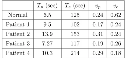
As the 2CFM is typically applied to renal data, a repre-sentative set of five whole-kidney tissues were defined: one
representing normal kidneys with parameter values mea-sured in healthy volunteers (6), and four pathological kid-neys taken from a recent patient study (21). Cases were selected by identifying the kidneys corresponding to the 10th and 90th percentiles in Te and vp. The parameters
are summarised in Table 1.
Tp (sec) Te (sec) vp ve
[image:5.612.316.525.137.234.2]Normal 6.5 125 0.24 0.62 Patient 1 9.5 102 0.17 0.24 Patient 2 13.9 153 0.31 0.24 Patient 3 7.27 117 0.19 0.26 Patient 4 10.3 214 0.29 0.18
Table 1: Parameter values of the simulated data sets.
To generate an exact ground-truthC(t), one of the five tissue types was selected at random with equal proba-bility, and C(t) was calculated with the analytical solu-tion (Eq.[7]). A literature-based arterial input funcsolu-tion
ca(t) was used (22), prepadded with zeroes to create a
20s baseline. C(t) and ca(t) were created at a
pseudo-continuous temporal resolution of 10msec for times rang-ing fromt= 0sto a total ofTacq = 300s. All convolutions
in this study are calculated using a formula that is op-timised for convolutions with an exponential factor (see Appendix).
Measurements with a given uniform sampling interval TR (sec) and Contrast-to-Noise Ratio (CNR) were simu-lated. CNR is defined in this study as the ratio of peak arterial concentration to the standard deviation (SD) of the noise, ie. CNR = max(ca)/SD. In DCE-MRI this is a
better measure for the noise level than SNR as the analy-sis is performed on signal changes rather than on absolute signal values. The first time-pointt0 of the measurement was determined by selecting a random number from a uni-form distribution on the interval [0,TR]. Then time-points
tn = t0+nTR were added with n = 1, . . . , N −1 and
N = ⌊Tacq/TR⌋. Downsampled C(tn) and ca(tn) were
us-ing the trapezoidal rule. The least-squares system was solved by inverting the 4×4 normal equations, i.e. X = (ATA)−1ATC. The NLLS was implemented by
fit-ting the analytical solution (Eq.[7]) using the Levenberg-Marquardt algorithm with the functionMPFIT(23). Con-volutions were calculated with the iterative formula in the Appendix. Partial derivatives with respect to the model parameters were calculated numerically and default values were used for the termination tolerance (10−3) and
max-imum number of iterations (200). No constraints were placed on any of the parameters, and fixed initial values were used. They were taken at approximately half the ex-act values in normal tissue to avoid a bias with respect to a particular tissue type (Tp = 3s, Te = 60s, vp = 0.1,
ve= 0.3).
For each reconstructionPi of a parameterP =Fp,P S,
Tp,Te, the errorEi(P) was determined as a percentage of
the exact value:
Ei(P) = 100∗
Pi−P
P [25]
The goodness-of-fit was quantified in a similar way as the relative distance between the fitted concentrationsCfit
i (tn)
and measured concentrationsCmsr
i (tn):
Ei(C) = 100∗
kCfit
i −Cimsrk2
kCmsr
i k2 [26]
Simulations for given TR and CNR were repeated 10,000 times to determine the distribution of results. The median relative errorE50was recorded as a measure of the system-atic error, and the 90% confidence interval CI =E95−E5
as a measure of the random error.
The performance of the LLS or WLLS was quantified via two figures of merit (FoM), one for the accuracy and one for the precision:
FoM (Accuracy) =|E50(NLLS)| − |E50(LLS)| [27]
FoM (Precision) = CI(NLLS)−CI(LLS) [28]
A positive (negative) FoM means that the LLS improves (reduces) the accuracy or precision. Numerically, a FoM of 1% implies that LLS reduces the systematic or random error by 1% of the exact parameter value. FoM’s were determined explicitly for 3 different protocols:
• Protocol 1 (CNR=50 and TR=1.25s) models single-voxel data at high temporal resolution (and thus high noise levels).
• Protocol 2 (CNR=10000 and TR=12.5s) models ROI data at low temporal resolution (and thus low noise levels).
• Protocol 3 (CNR=10000 and TR=1.25s) models ideal conditions of high temporal resolution and low noise levels.
Protocol 1 and 2 represent realistic boundary regimes, and may be used to measure Fp-maps (protocol 1) or
ROI-based P S (protocol 2). Protocol 3 represents a limiting case of error-free data that cannot be realised in practice but is useful to help understand the fundamental behavior of the methods. Realistic CNR and TR values for proto-col 1 were estimated by measurement on a patient data set acquired with a standard 2D acquisition protocol (6). Values for protocol 2 were estimated on the same data after time-averaging to a TR of 12.5s.
RESULTS
Figure 2 provides an illustration of the data and model fits at the highest noise level considered in this study. The plots show that the fit to the data is significantly poorer with LLS than with NLLS, which provides an almost ex-act reconstruction of the underlying concentrations de-spite high levels of noise.
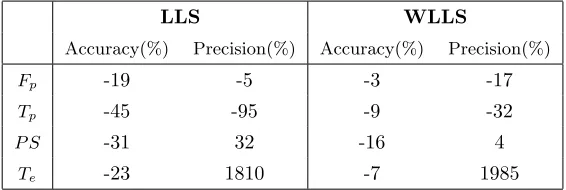
Table 2 provides the FoM’s under the conditions of high noise and high temporal resolution (protocol 1). In this regime the LLS is associated with a significant loss in accu-racy in all parameters (−30% on average). Adding weight-ing improves the accuracy in all parameters, but it is still lower than with NLLS (−9% on average). The effect on precision depends on the parameter: LLS causes a major loss in precision forTp(−95%),but improves the precision
forP SandTe. In this case the weighting has a benefit as
it reduces the loss in precision for Tp. But the effect
Table 3 provides the FoM’s under the opposite condi-tions of low noise and low temporal resolution (protocol 2). Under these conditions the LLS shows a clear improve-ment in accuracy (+10% on average) and precision in all parameters. In this particular scenario there is no numer-ical benefit in adding a weighting withW(t) =ca(t). The
gain in precision is +4763% on average, but this is largely determined by an outlier (Te). Excluding this, the gain in
[image:7.612.295.578.75.170.2]precision is still +129% on average.
Table 4 provides the FoM’s under the ideal circum-stances of protocol 3 (low noise and high temporal resolu-tion). The results show that LLS leads to small changes in both accuracy (0.1% improvement on average) and pre-cision (0.1% loss on average). As for protocol 2 there is no numerical benefit in adding a weighting withW(t) =ca(t)
in this particular scenario.
Figure 3 shows that the differences in accuracy and precision are small under the ideal conditions of proto-col 3. The distinction between LLS and NLLS is most pronounced in the parameter Fp, where NLLS and LLS
produce relative errors in the range 0.4% ±0.6% and 0.2%±0.4%, respectively (median±half of 90% CI).
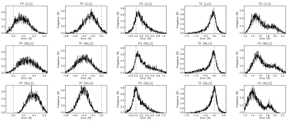
Figure 4 visualises the transition in the low-noise regime from protocol 3 (high temporal resolution) to protocol 2 (low temporal resolution) in more detail. The figure shows that the improved accuracy and precision of the LLS per-sists across the whole range of temporal resolutions, be-coming gradually more pronounced towards protocol 2 at the low temporal resolution (right side of the plot).
Figure 5 visualises the transition in the high temporal resolution regime from protocol 3 (low noise) to protocol 1 (high noise). The figure shows that the errors increase in a systematic manner with CNR, showing the stronger noise-sensitivity of LLS. For a measurement targeting the vascular parametersFpandTp, the NLLS is more reliable
at all noise levels. The NLLS is also preferred for the permeability parameters P S and Te, except in the
high-noise limit of protocol 1 where the WLLS is the optimal. Regarding the calculation time, the LLS method is faster than the NLLS method by a factor of 200, i.e. two orders of magnitude. In absolute terms, for an MR im-age of 256×256 pixels the computation time on a laptop
PC is 3 sec and 9 min for the LSS and NLLS methods, respectively.
LLS WLLS
Accuracy(%) Precision(%) Accuracy(%) Precision(%)
Fp -19 -5 -3 -17
Tp -45 -95 -9 -32
P S -31 32 -16 4
[image:7.612.294.579.243.336.2]Te -23 1810 -7 1985
Table 2: Figures of Merit (FoM) for LLS and WLLS for pro-tocol 1 at high noise level (CNR=50) and high temporal reso-lution (TR=1.25s).
LLS WLLS
Accuracy(%) Precision(%) Accuracy(%) Precision(%)
Fp 14 265 -14 122
Tp 13 49 -13 -242
P S 7 74 6 -40
Te 6 18664 -0.1 18680
Table 3: Figures of Merit (FoM) for LLS and WLLS for pro-tocol 2 at low noise level (CNR=10000) and low temporal res-olution (TR=12.5s).
LLS WLLS
Accuracy(%) Precision(%) Accuracy(%) Precision(%)
Fp 0.27 -0.11 0.1 -0.2 Tp 0.15 -0.14 0.01 -0.2 P S -0.01 -0.1 -0.13 -0.2 Te -0.01 -0.1 -0.07 -0.3
Table 4: Figures of Merit (FoM) for LLS and WLLS for pro-tocol 3 under ideal conditions of low noise level (CNR=10000)
and high temporal resolution (TR=1.25s).
DISCUSSION
Figure 2: : Example of simulated data for single-voxel curve (protocol 1) at TR=1.25s and CNR=50. (a) The figure shows results in the arterial plasma. The dashed line represent the exact concentration. The insert gives the Figures of Merit for each of the parameters in this particular case. (b) The figure shows results in the tissue with an overlay of the LLS fit (full line). The dashed line represent the exact concentration and the diamonds indicate the simulated measurements. (c) The figure
shows results in the tissue with an overlay of the NLLS fit (full line). The dashed line represent the exact concentration and the diamonds indicate the simulated measurements.
[image:8.612.50.543.385.594.2]Figure 4: Error distribution at fixed CNR=10000 (low noise level) but variable TR. The circles indicate the median error and the error bars represent the 90% confidence interval. Results are shown for each method (LLS - top row, WLLS - middle row, NLLS - lower row) and for each parameter (Fp - column 1, Tp - column 2, P S - column 3, Te column 4, goodnessoffit -column 5).
[image:9.612.45.542.383.591.2]data. It also depends on the implementation of the NLLS. In this study a fixed initial value was used rather than a grid of initial values, and in that sense the estimate of NLLS calculation time represents a best case scenario. The improvement in calculation time is not of practical significance for a ROI-based analysis, where other steps in the analysis form the main bottlenecks (e.g. data trans-fer, segmentation). However for a pixel-based analysis the improvement may have significant implications for clini-cal practice. The effect may also be important for other methods that use pixel-based tracer-kinetic modeling as an intermediate step, such as model-based segmentation or registration techniques, or data undersampling strate-gies using the temporal structure as a constraint.
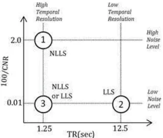
The effect of LLS on accuracy and precision is more ambiguous. Key observations are summarised in Figure 6. As a general rule, the LLS is preferred at low-noise conditions and the NLLS at high temporal resolution. In the ideal conditions where these two regimes meet (proto-col 3), their performance is comparable and both can be used interchangeably. The NLLS is slightly more reliable as the gain in precision offsets the loss in accuracy, but the differences are small and not likely to be significant for clinical applications. In that sense, the LLS may be preferred in view of its computational benefit. There is no benefit of adding a weighting with W(t) = ca(t)
ex-cept for the leakage parameters under conditions of very high noise and high temporal resolution (protocol 1). This regime is less relevant as all measurements are unreliable under these conditions. For the same reasons the regime of low temporal resolution and high noise level is not of practical interest (upper right corner of Fig.6).
The systematic error of the LLS at higher noise levels is unexpected from an MRI perspective as previous ex-periences with the linearised extended Tofts model have shown an improved accuracy at higher noise levels (11,25). In part, this discrepancy may be due to implementation differences in the NLLS between the current and previ-ous studies (11). However, it is likely that the effect is mostly due to the added complexity of a 2nd-degree linear model. A key difference with the extended Tofts model is that the linearised equation of the 2CXM or 2CFM
con-Figure 6: Summary of the observations regarding accuracy and precision. The figure maps different experimental
condi-tions in the TR - CNR plane showing the location of the three protocols for which the Figures-of-Merit have been simulated
(circles) and the different limiting regimes of high/low noise level and high/low temporal resolution (dotted lines). Opti-mal choices of methods (NNLS, LLS) are indicated next to the
respective protocols.
tains a second-order derivative. This leads to the double integrals in Eq.[18] which effectively add a strong weight on the later time points where little temporal structure is available. As a result the solution becomes less well determined than in the NLLS, where the first-pass data carry a strong weight due to the high signal values in this regime. This is also consistent with the observation that a weighting factor W(t) = ca(t) reduces the systematic
errors significantly: at high temporal resolution the func-tion ca(t) is dominated by the first pass where most of
the temporal structure can be found. The chosen weight-ing does not remove the error completely, but alternative weighting strategies have not been explored and could lead to further improvement. An alternative solution that may be worth considering is the use of the differential form combined with temporal filtering to reduce the noise sen-sitivity (25). However, it is not clear whether this remains beneficial in second order.
[image:10.612.341.501.54.190.2]cause a bias in the parameters (9, 16, 17, 20, 26, 27). There is no a priori guarantee that these observations translate to DCE-MRI (or DCE-CT). Noise levels, temporal resolu-tions and acquisition times generally lie in entirely differ-ent regimes. A more fundamdiffer-ental difference lies in the typ-ical data structure of first-pass DCE-MRI or -CT, where all high-frequency information is stored in a narrow and early time interval. This explains why the weighting effect of the double integration is more significant in DCE-MRI. Nevertheless, our study confirms that LLS at high noise levels causes a bias in all DCE-MRI parameters.
This raises the question of whether the solutions pro-posed for PET could help to reduce the bias. Feng et al. (9, 17) proposed a generalized linear least squares (GLLS) method, which has found some use in pixel-based param-eter estimation for PET (28). However a more recent comparative study indicated that it still exhibits large bias and poor precision at higher noise levels (20). Zeng et al. (19) proposed a more general weighted integration method to address the problem. Instead of integrating the linear equation (Eq.[11]) twice over time, it is multiplied with wavelets g(t, T) on a support t ∈ [0, T], and inte-grated once over that interval. Despite appearances, this method is not fundamentally different from double inte-gration, and it is identical when the wavelets are chosen asg(t, T) =T −t. This follows from the identity:
Z T
0
dt(T−t)f(t) = ¯¯f(T) [29]
Hence, one would not expect an improved performance. Zeng et al. (19) did not observe a bias, but the scope of their simulations was limited and restricted to data with low temporal resolution and relatively low noise levels. This corresponds roughly to the low-noise regime where we have also observed that the LLS is more robust (lower right corner of Fig.6). The wavelet-based method does have the advantage that different families of wavelets can be used, but there is no evidence that this would eliminate the observed bias.
Another question that could be asked is whether the LLS problem suffers from ill-posedness and could bene-fit from regularisation. At first glance the strong noise sensitivity of a parameter likeTe could be seen as an
in-dication thereof, but the problem appears in the NLLS as well. In this case the sensitivity of Te most likely
re-flects a limitation of the data: the “population” contains a case (patient 4) with aTe-value (214s) that is relatively
close to the acquisition time Tacq (300s). In that case the washout of tracer is not well-resolved and its transit time cannot be determined reliably except with ideal noise-free data. As part of the development process it was also eval-uated whether the errors could be improved by regular-ising the solution using truncated singular value decom-position. We found that this only introduced systematic error, which indicates that the problem is not ill-defined (data not shown).
to LLS methods as well.
CONCLUSION
The LLS method for solving the 2CXM or 2CFM reduces the computation times by two orders of magnitude, and is at least as accurate and precise as the NLLS at low noise levels. At higher noise levels the LLS becomes exceed-ingly inaccurate compared to the NLLS, but this may be improved by using a suitable weighting strategy.
Acknowledgments
This study was supported by a CASE studentship of the Engineering and Physical Sciences Research Council (EPRSC) and GlaxoSmithKline (GSK).
Appendix
The NLLS implementation in this study uses an efficient and accurate iterative algorithm for the evaluation of a convolutions with an exponential factor:
f(t) =a(t)⊗e
−t/T
T ≡
1
T
Z t
0
dτ a(τ)e−(t−τ)/T [A1]
The algorithm applies to situations where the function
a(t) is measured and thus only available at discrete times
t0= 0, t1, t2, . . . , tn−1 (not necessarily uniformly spaced).
With T = 0 the result is f(t) = a(t). With T 6= 0 the integral is evaluated by interpolating linearly between the valuesai=a(ti), leading to an iterative formula with
starting valuef(t0) = 0:
f(ti+1) =e−xif(ti) +aiE0(xi) +a′iT E1(xi) [A2]
where
E0(x) =
Z x
0
e−(x−u)du= 1−e−x [A3]
E1(x) =
Z x
0
ue−(x−u)du=x−E0(x) [A4]
and
xi≡
ti+1−ti
T , a ′
i≡
ai+1−ai
ti+1−ti
[A5]
Compared to standard numerical convolution, Eq. [A2] is more accurate because the exponential factor is not ap-proximated. It is also more efficient computationally due to its iterative nature.
To prove the results, consider first the caseT = 0:
lim
T→0 e−t/T
T ∗a(t) =δ(t)∗a(t) =a(t) [A6]
For any other T, note that the initial value is f(t0) = 0 since t0 = 0. Now given f(ti), the value f(ti+1) can be
determined by splitting up the integral and substituting
u= (τ−ti)/T:
1
T
Z ti+1
0
dτ a(τ)e−(ti+1−τ)/T
= 1
T
Z ti
0
dτ a(τ)e−(ti+1−τ)/T
+ 1
T
Z ti+1
ti
dτ a(τ)e−(ti+1−τ)/T
= 1
T
Z ti
0
dτ a(τ)e−xi−(ti−τ)/T
+
Z xi
0
du a(ti+T u)e−(xi−u)
≈ e−xif(t
i) + Z xi
0
du(ai+a′iT u)e
−(xi−u)
References
[1] Sourbron SP, Buckley DL. Tracer kinetic modelling in MRI: estimating perfusion and capillary permeability. Phys Med Biol 2012;57: R1−R33.
[2] Tofts PS, Brix G, Buckley DL, et al. Estimating kinetic parameters from dynamic contrast-enhanced T1-weighted MRI of a diffusable tracer: Standard-ized quantities and symbols. J Magn Reson Imaging 1999;10:223−232.
[3] Patlak CS, Blasberg RG. Graphical evaluation of blood-to-brain transfer constants from multiple-time uptake data. Generalizations. J Cereb Blood Flow Metab 1985;5:584−590.
[4] Brix G, Kiessling F, Lucht R, Darai S, Wasser K, De-lorme S, Griebel J. Microcirculation and microvas-culature in breast tumors: pharmacokinetic analy-sis of dynamic MR image series. Magn Reson Med 2004;52:420−429.
[5] Annet L, Hermoye L, Peeters F, Jamar F, Dehoux JP, Van Beers BE. Glomerular filtration rate: assessment with dynamic contrast-enhanced MRI and a cortical-compartment model in the rabbit kidney. J Magn Re-son Imaging 2004;20:843−849.
[6] Sourbron SP, Michaely HJ, Reiser MF, Schoenberg SO. MRI-measurement of perfusion and glomerular filtration in the human kidney with a separable com-partment model. Invest Radiol 2008;43:40−48.
[7] Ahearn TS, Staff RT, Redpath TW, Semple SI. The use of the Levenberg-Marquardt curve-fitting algo-rithm in pharmacokinetic modelling of DCE-MRI data. Phys Med Biol 2005;50:N85−N92.
[8] Chen H, Li F, Zhao X, Yuan C, Rutt B, Ker-win WS. Extended graphical model for analysis of dynamic contrast-enhanced MRI. Magn Reson Med 2011;66:868−878.
[9] Feng D, Wang ZZ, Huang SC, Wang ZZ, Ho D. An unbiased parametric imaging algorithm for
nonuni-formly sampled biomedical system parameter estima-tion. IEEE Trans Med Imaging 1996;15:512−518.
[10] Leporq B, Camarasu-Pop S, Davila-Serrano E, Pilleul F, Beuf O. Enabling 3D-Liver perfusion mapping from MR-DCE imaging using distributed computing. J Med Eng 2013;471682.
[11] Murase K. Efficient method for calculating kinetic parameters using T1-weighted dynamic contrast-enhanced magnetic resonance imaging. Magn Reson Med 2004;51: 858−862.
[12] C´ardenas-Rodr´iguez J, Howison CM, Pagel MD. A linear algorithm of the reference region model for DCE-MRI is robust and relaxes requirements for temporal resolution. J Magn Reson Imaging. 2013;31:497−507.
[13] Li J, Yu Y, Zhang Y, Bao S, Wu C, Wang X, Li J, Zhang X, Hu J. A clinically feasible method to es-timate pharmacokinetic parameters in breast cancer. Aapm. 2009;36:3786−3794.
[14] Adluru G, DiBella EV, Schabel MC. Model-based registration for dynamic cardiac perfusion MRI. J Magn Reson Imaging 2006;24:1062−1070.
[15] Faranesh AZ, Kraitchman DL, McVeigh ER. Mea-surement of kinetic parameters in skeletal muscle by magnetic resonance imaging with an intravascular agent. J Magn Reson Medicine 2006;55:1114−1123.
[16] Wen L, Eberl S, Fulham MJ, Feng D, Beng J. Con-structing reliable parametric images using enhanced GLLS for dynamic SPECT. IEEE Trans Biomed Eng 2010;56:1117−1126.
[17] Feng D, Ho D, Chen K, Wu LC, Wang JK, Liu RS, Yeh SH. An evaluation of the algorithms for deter-mining local cerebral metabolic rates of glucose using positron emission tomography dynamic data. IEEE Trans Med Imaging 1995;14:697−710.
Science Symposium and Medical Imaging Conference Record 2011;3209−3216.
[19] Zeng GL, Hernandez A, Kadrmas DJ, Gullberg GT. Kinetic parameter estimation using a closed-form ex-pression via integration by parts. Phys Med Biol 2012;57:5809−5821.
[20] Dai X, Chen Z, Tian J. Performance evaluation of kinetic parameter estimation methods in dynamic FDG-PET studies. Nucl Med Commun 2011;32:4−16.
[21] Lim SW, Chrysochou C, Buckley DL, Kalra PA, Sourbron SP. Prediction and assessment of re-sponses to renal artery revascularization with dy-namic contrast-enhanced magnetic resonance imag-ing: a pilot study. Am J Physiol Renal Physiol 2013;305:672−678.
[22] Parker GJ, Roberts C, Macdonald A, et al. Experimentally-derived functional form for a population-averaged high-temporal-resolution arte-rial input function for dynamic contrast-enhanced MRI. Magn Reson Med 2006;56:993−1000.
[23] Markwardt, CB. Non-Linear Least Squares Fitting in IDL with MPFIT. In: Proceedings Astronom-ical Data Analysis Software and Systems XVIII 2009;411:251−254.
[24] Veraart J, Sijbers J, Sunaert S, Leemans A, Jeurissen B. Weighted linear least squares estimation of diffu-sion MRI parameters: Strengths, limitations and pit-falls. NeuroImage 2013;81:335−346.
[25] Wang C, Yin F-F, Chan, Z. An efficient calcula-tion method for pharmacokinetic parameters in brain permeability study using dynamic contrast-enhanced MRI. Magn Reson Med. 2015. Online ahead of print.
[26] Cai W, Feng D, Fulton R, Siu W-C. Generalized linear least squares algorithms for modeling glucose metabolism in the human brain with corrections for vascular effects. Comput Methods and Programs Biomed 2002;68:1−14.
[27] Ichise M, Toyama H, Innis RB, Carson RE. Strategies to improve neuroreceptor parameter estimation by linear regression analysis. J Cereb Blood Flow Metab 2002;22:1271−1281.
[28] Chen K, Lawson M, Reiman E, et al. General-ized linear least squares method for fast genera-tion of myocardial blood flow parametric images with N-13 ammonia PET. IEEE Trans Med Imaging 1998;17:236−243.
[29] Banks HT, Dediu S, Ernstberger SL. Sensitivity func-tions and their use in inverse problems. Inv Ill-posed problems 2007;15:683-708.