Article:
Gilbert, AD, Mason, J and Tobias, SM (2016) Flux expulsion with dynamics. Journal of
Fluid Mechanics, 791. pp. 568-588. ISSN 0022-1120
https://doi.org/10.1017/jfm.2016.60
eprints@whiterose.ac.uk https://eprints.whiterose.ac.uk/ Reuse
Unless indicated otherwise, fulltext items are protected by copyright with all rights reserved. The copyright exception in section 29 of the Copyright, Designs and Patents Act 1988 allows the making of a single copy solely for the purpose of non-commercial research or private study within the limits of fair dealing. The publisher or other rights-holder may allow further reproduction and re-use of this version - refer to the White Rose Research Online record for this item. Where records identify the publisher as the copyright holder, users can verify any specific terms of use on the publisher’s website.
Takedown
If you consider content in White Rose Research Online to be in breach of UK law, please notify us by
Flux expulsion with dynamics
Andrew D. Gilbert
1, Joanne Mason
1and Steven M. Tobias
21Department of Mathematics and Computer Science, College of Engineering, Mathematics and Physical Sciences, University of Exeter, EX4 4QF, UK
2Department of Applied Mathematics, University of Leeds, LS2 9JT, UK
(Received xx; revised xx; accepted xx)
In the process of flux expulsion, a magnetic field is expelled from a region of closed streamlines on a T R1m/3 time scale, for magnetic Reynolds number Rm ≫ 1 (T being the turnover time of the flow). This classic result applies in the kinematic regime where the flow field is specified independently of the magnetic field. A weak magnetic ‘core’ is left at the centre of a closed region of streamlines, and this decays exponentially on the
T R1m/2 time scale.
The present paper extends these results to the dynamical regime, where there is compe-tition between the process of flux expulsion and the Lorentz force, which suppresses the differential rotation. This competition is studied using a quasi-linear model in which the flow is constrained to be axisymmetric. The magnetic Prandtl numberRm/Re is taken to be small,Rmlarge, and a range of initial field strengthsb0 is considered.
Two scaling laws are proposed and confirmed numerically. For initial magnetic fields below the threshold bcore = O(U R−m1/3), flux expulsion operates despite the Lorentz force, cutting through field lines to result in the formation of a central core of magnetic field. Here U is a velocity scale of the flow and magnetic fields are measured in Alfv´en units. For larger initial fields the Lorentz force is dominant and the flow creates Alfv´en waves that propagate away. The second threshold isbdynam =O(U R−m3/4), below which the field follows the kinematic evolution and decays rapidly. Between these two thresholds the magnetic field is strong enough to suppress differential rotation leaving a magnetically controlled core spinning in solid body motion, which then decays slowly on a time scale of orderT Rm.
1. Introduction
Throughout the universe electrically conducting fluid flows interact with magnetic fields. By the stretching and folding of magnetic field lines, initially weak fields can grow, a pro-cess known as dynamo action (Moffatt 1978). As the magnetic field increases in strength it then resists deformation through Lorentz forces exerted on the flow. Eventually a state of fully developed MHD turbulence ensues, composed of a superposition of coherent structures and random eddies interacting with magnetic fields.
Motivation for this approach comes from the study of the coupling of magnetic fields and convection (Weiss & Proctor 2014); furthermore in rapidly rotating convection the dynamics may be dominated by long-lived coherent structures taking the form of vortices (Julienet al.2012). The problem has been addressed in a kinematic regime in which the magnetic field is presumed to be so weak as not to affect the flow, which may then be specified and ceases to have any dynamical attributes. This classic problem was first studied for a smooth flow in the pioneering numerical study of Weiss (1966), and by Parker (1966) for the case of a piecewise smooth flow. These works led to identification of the fundamental process of flux expulsion, whereby the field is destroyed within regions of closed streamlines; in cellular flows the resulting magnetic fluxes are then concentrated on bounding separatrices.
The mathematical theory of flux expulsion is elucidated for linear and axisymmetric, smooth flow fields by Moffatt & Kamkar (1983) and for more general streamline geometry by Rhines & Young (1983). The effect of a closed eddy on a weak imposed field at high magnetic Reynolds numberRm(that is,U L/η whereU is the characteristic flow speed,
L is a characteristic length and η is the magnetic diffusivity) is to expel field towards the cell boundaries on a time scale of orderT R1m/3, whereT =L/U is the turnover time scale. The key mechanism is the effect of shear or differential rotation in reducing length scales and so accelerating diffusion, be it of magnetic vector potential, passive scalar or vorticity: the useful and general term shear–diffuse mechanism was coined by Bernoff & Lingevitch (1994). These studies are elaborated in Bajer (1998) and Bajer, Bassom & Gilbert (2001), referred to as BBG in what follows. In BBG a further time scale is identified at the eddy centre: here any differential rotation must vanish for a smooth flow, and the shear–diffuse process is weaker. The flux expulsion time scale here increases to order T R1m/2 and a weak remnant, which we will call a magnetic core, is created and decays exponentially on this time scale.
Our goal in the present paper is to extend these kinematic studies into the dynamical regime, in which the field affects the flow via the Lorentz force. While it is clear that for sufficiently weak magnetic fields kinematic results are recovered, we address the question of the threshold for the field to have a dynamical effect for the classic problem of flux expulsion in an axisymmetric flow. From another viewpoint, the question becomes: for what field strengths (in a two-dimensional flow) will a magnetic field have an impact on the material conservation of vorticity? Many interesting dynamical effects in quasi two-dimensional hydrodynamics in rotating systems, such as zonal flow generation, have been ascribed to the material conservation properties of potential vorticity (Dritschel & McIntyre 2008). It is therefore critical for MHD studies to determine the effect of magnetic fields in modifying these conservation properties. It is known that such dynamical effects of the magnetic field can be subtle, and depend sensitively on molecular values of the transport coefficients. Perhaps the key study that highlights this is Cattaneo & Vainshtein (1991): the authors consider transport in turbulent two-dimensional fluid flows with a mean magnetic fieldb0 across the system. For field strengths b0 (in Alfv´en
energy or enstrophy in three- or two-dimensional turbulence. Similar effects arise in magnetoconvection (Galloway, Proctor & Weiss 1978; Weiss & Proctor 2014), in which flux expulsion drives magnetic flux to the boundary of convective cells. In dynamical regimes, the resulting peak fields are limited not by equipartition values b0 = O(U)
but can be substantially larger, with dependence on the magnetic diffusivity and fluid viscosity.
To address the problem of dynamical effects and thresholds for flux expulsion, in this paper we will work in the most straightforward setting of a flow with initially circular streamlines permeated by a uniform magnetic field of strengthb0. The problem is set up
in section 2, parameterised byb0 and values of the magnetic Reynolds numberRmand (fluid) Reynolds numberRe. We will work in the quasi-linear approximation in which we keep the fluid flow axisymmetric and truncate the Lorentz force feedback by retaining only the mean azimuthal component. This is reasonable as we are examining the onset of the importance of the Lorentz force in the dynamics. The approach can be justified in some contexts such as dynamos in high Reynolds number rotating flow (as we have here)†(Bassom & Gilbert 1997) and transport and jet formation in geophysical systems, for example see Tobias, Dagon & Marston (2011) and Srinivasan & Young (2012).
In section 3 of the paper we present numerical simulations of the evolution of field and flow (within the quasi-linear model) for a range of initial magnetic field strengths. Here we observe the key competition or race between the processes of flux expulsion and Lorentz force feedback: will the Lorentz force act early enough to halt the stretching in the flow and so defuse the dramatic effect of flux expulsion in destroying the field? Or, will flux expulsion act first and cut elastic field lines so as to remove the Lorentz force feedback and leave a magnetic core behind? We work in a regime in whichRe≫Rm≫1 to highlight the transition between these effects without consideration of viscosity, and this gives us our first thresholdbcore(η) forb0, as discuss below. However we also obtain
a second, lower thresholdbdynam(η), below which the magnetic field has no discernible
effect and the kinematic picture holds. In sections 4 and 5 we develop the theory for the two thresholds identified in section 3, based both on the classic asymptotics in Moffatt & Kamkar (1983) and Rhines & Young (1983), and on the more elaborate picture in BBG, which we need to identify the lower threshold. Finally section 6 offers some concluding comments and avenues for further research.
2. Governing equations
Our starting point is the equations for MHD, written in the form
∂tu+u· ∇u=b· ∇b− ∇p+ν∇2u, (2.1)
∂tb+u· ∇b=b· ∇u+η∇2b, (2.2)
∇ ·u=∇ ·b= 0. (2.3)
The two-dimensional flow and field(measured in velocity units)are confined to the plane
z= 0 in cylindrical polar coordinates (r, θ, z), and setting u=∇ ×(ψzˆ), b=∇ ×(aˆz) we obtain the equations in terms of the stream functionψ, vorticityω, flux functiona,
† Note that in a rotating fluid flow, the axisymmetric component of the Lorentz force
and currentj, all functions of (r, θ, t), as
∂tω=J(ψ, ω)−J(a, j) +ν∇2ω, (2.4)
∂ta=J(ψ, a) +η∇2a, (2.5)
ω=−∇2ψ, j=−∇2a. (2.6)
Here the Jacobian is given byJ(ψ, ω) =r−1[(∂
rψ)(∂θω)−(∂θψ)(∂rω)].
Following the discussion in Moffatt & Kamkar (1983), we commence with an initial uniform magnetic field in thex-direction and an axisymmetric flow field. Thusψand ω
are taken to be independent ofθ and the fields a and j are represented using an eimθ dependence withm = 1. Although our focus is always on m = 1, it is helpful in the analytical development to leave a general, integer value ofm >0. We therefore set for the flow
ω=ω(r, t) +· · ·, ψ=ψ(r, t) +· · · , (2.7)
and for the field
a= ˜a(r, t)eimθ+ c.c.+· · ·, j= ˜j(r, t)eimθ+ c.c.+· · · , b= ˜b(r, t)eimθ+ c.c.+· · ·. (2.8)
The tildes denote the harmonic m >0 in θ, but for readability we drop these in what follows.
Now the Lorentz force feedback from the field to the flow will incorporate a mean part, independent ofθ, and harmonics e2imθ, which will then proliferate, giving the trailing terms not written down explicitly in (2.7, 2.8). We employ a truncation by neglecting these higher order harmonics, and retain only the terms shown. This leaves the quasi-linear system for the field harmonicmand the mean flow, written compactly as
∂ta+imα a=η∆ma, (2.9)
∂tω=r−1∂rG+ν∆0ω. (2.10)
The angular velocity isα(r, t) =−r−1∂
rψ, and the current and vorticity are linked by
j=−∆ma, ω=−∆0ψ, (2.11)
where∆m=∂r2+r−1∂r−m2r−2. The Lorentz force term in (2.10) isG(r, t) given by
G=im(aj∗−a∗j). (2.12)
We will use this quasi-linear approximation to gain an understanding of the essential pro-cesses in the competition between flux expulsion and the Lorentz force, both numerically and analytically.
For initial conditions, our focus is on the case of a uniform field in thex-direction of strengthb0, which has currentj = 0. However we generalise to an arbitary value of m,
and consider an initial multipole, current-free field given by the vector potential
a(r,0) =−1
2ib0r
m (2.13)
(with b0 real). We also need an initial axisymmetric fluid flow u and have chosen a
Gaussian vortex with
ω(r,0) =T−1(4π)−1e−r2/4L2, α(r,0) =T−1(2πr2/L2)−1(1−e−r2/4L2). (2.14)
whereLis a length scale,T a time scale, and belowU =L/T. We will non-dimensionalise the system using these scales and defining, for example:
r
2 4 6 8 10
α
(
r
)
,
α
′(r
)
-0.01 -0.005 0 0.005 0.01 0.015 0.02 0.025 0.03 0.035
[image:7.612.214.394.100.247.2]1.8
Figure 1.The angular velocity profileα(solid) in (2.16) andα′(dashed), with the location of
maximal differential rotation|α′|identified asr†≃1.8.
with hats denoting non-dimensional quantities. With this we can also identifyRm≡ηˆ−1
as a magnetic Reynolds number, Re ≡ νˆ−1 as a Reynolds number and M ≡ ˆb−01 as a magnetic Mach number. We will in what follows drop the hats and work with dimensionless quantities, except when we refer to our results in the final discussion section.
Our goal then is to solve the PDEs specified in (2.9–2.12), for the initial conditions (2.13) and now
ω(r,0) = (4π)−1e−r2
/4, α(r,0) = (2πr2)−1(1−e−r2
/4). (2.16)
The angular velocityαand differential rotationα′≡∂
rαare depicted in figure 1, where for convenience we often use a prime to denote a radial derivative.The radiusr† marks the location of maximal differential rotation |α′|, where we will see that flux expulsion commences in a kinematic regime.
The parameter set comprises the three non-dimensional quantities {η, ν, b0}, and we use this form as it is more convenient to place “η” rather than the bulky term “R−1
m”
in our calculations.We are interested in the regimes that are realised depending on the strength of the initial field for different diffusive parameters. In this study our primary interest is in the interaction of flux expulsion (depending onη) and the Lorentz force (linked to b0), rather than viscous effects. We will thus take ν ≪ η and so work at a
low value of the magnetic Prandtl numberPm≡Rm/Re=ν/η.†In all the simulations shown, we have simply takenPm= 0.01, and tests confirm that our results are insensitive to this precise value. Our parameter set is thus reduced to{η, b0} and we are interested
in thresholds for different types of behaviour, givingb0 as a function of η with a power
law scaling: how strong must the initial field be for the Lorentz force to modify the classic picture of flux expulsion?
Theory for these thresholds is developed in section 4. Before giving numerical results in the next section though, it is worthoutlining the origin of theclassic approximation for kinematic flux expulsion (for more detail see Moffatt & Kamkar (1983), Rhines & Young (1983)).Consider when there is no dissipation, then the vector potential and current are
† Note that viscous damping would emerge on a time scale of order Re whereas the effects
we consider occur on time scales of orderR1m/3 and R1m/2, and thus our results are likely to be
given by
a=−12ib0rme−imαt, j≃ −21ib0rmm2α′2t2e−imαt, (2.17)
where we have retained inj just the terms that grow fastest, that is quadratically with timet. For small η, then, the right-hand sideη∆ma=−ηj in (2.9) grows quadratically
from small values and the accumulated effect of the dissipation gives a term cubic int. Incorporating this damping in the evolution ofathen yields the approximate solution
a≃ −12ib0rme−imαt−
1
3ηm
2
α′2
t3
, j≃ −12ib0rmm2α′2t2e−imαt−
1
3m
2
ηα′2
t3
. (2.18)
This gives dramatic suppression of the vector potential and so of the magnetic field, which commences at the radiusr† where|α′|is maximised, indicated on figure 1 for the Gaussian profile (2.16), on a timescalet† =O(η−1/3).†Specificallyr† and t† (up to an order one constant) are given by
r†= arg max
r |α
′(r)|2, t†= [1 3m
2ηα′(r†)2]−1/3. (2.19)
The dagger helpfully denotes the cutting of magnetic field lines caused by flux expulsion. For our purposes there are two problems with this approximation. The first is that the Lorentz force term (2.12) vanishes identically to this order. The next order terms need to be taken into account, and we undertake this in a systematic development in section 4.2. The second issue is discussed in BBG and is that this approximation breaks down near the origin whereα′→0. In other words the approximation is predicated on a shearα′=O(1) that makes the quadratic multipliert2in j in (2.18) dominant; towards the centre of a vortex another, inner approximation has to be used. Although this may seem a technical issue, in fact it is key to understanding the dynamical problem, and we develop this in section 4.1 following BBG. In preparation for this we note here that the angular velocity in (2.16) behaves asr→0 according to
α=α0+α1r2+α2r4+· · ·, (2.20)
α0= 1/8π, α1=−1/64π. (2.21)
From the point of view of the kinematic problem, with the axisymmetric flow specified independent of the field, the form (2.20) gives the behaviour near the origin. Smoothness considerations eliminate any odd powers of r and generically the constant α1 is
non-zero. This constant plays an important role in kinematic theory as it controls how the differential rotation α′ responsible for flux expulsion switches off near the origin. Dynamically the magnetic field can change the form of the flow near the origin, as we shall see. We also note that the numerical values ofα0and particularlyα1≃ −1/200 are rather
low, meaning that the turnover time of the flow is large in our non-dimensionalisation and making the corresponding time scales appear long on our plots. For best comparison with simulations we will retain factors ofα1 in our theoretical development.
3. Numerical simulations
3.1. Illustrative runs
Our goal in this section is to present numerical simulations of the model (2.9–2.12) with the initial conditions (2.13, 2.16). This will motivate the theory in the next section, but we will also refer ahead to results in that section. Our parameters are only{η, b0}
(a) (b) (c)-2-2 -1.5 -1 -0.5 0 0.5 1 1.5 2 -1.5
[image:9.612.123.499.208.373.2]-1 -0.5 0 0.5 1 1.5
Figure 2.Kinematic magnetic field evolution. In (a,b)t= 104 and (c) 4×10⁴. In (a) −106x, y610, while in (b,c) only the central region−26x, y62 is depicted.
(a)
decaying eigenfunction
inner solution field destroyed
spiral wind-up
O(1) t
r r†
t†
O(η1/2) O(η−1/3) O(η−1/2)
(b)
104 105
10-12
10-10 10-8
10-6 10-4 10-2 100 102
Figure 3.(a) Schematic of kinematic evolution of magnetic field for η ≪1, and (b) log–log plot ofEM (upper solid) andEA(lower solid) as functions of timet. In (b) the scaling lawst−7
(4.10) andt−6(4.11) are depicted (dashed), and the formulae (4.13), (4.14) are shown (dotted).
and we first show the various phenomena that occur when we fixη= 10−7(withm= 1,
ν= 0.01η as always), and allow a range of values ofb0.
Our starting point is the kinematic problem when the field b0 is sufficiently weak
that dynamical effects may be neglected. Although the Lorentz force feedback is easily switched off in our simulations, one of our goals is to quantify just how weak the initial fieldb0needs to be for kinematic theory to apply, forη≪1. In any case we integrate (2.9)
in isolation. Figure 2 shows colour scale plots of the vector potential reconstructed from (2.8), so that lines of constant colour give magnetic field lines, from blue (low values ofa
in (2.8)) to red (high values); zero or weakais green. The panels show different times, and in each panel the colour scale is normalised separately on the maximum/minimum vector potential for that panel. Panel (a) gives a wide view, showing spiral wind-up of field lines by the flow and suppression of magnetic field by diffusion for moderater. Panels (b,c) show a zoom into the central region, where the onset of flux expulsion aroundr† can be seen in (b), followed by further destruction of field leading to the final phase in (c), of a decaying, remnant field structure localised at the origin.
Figure 3 shows a schematic of kinematic field evolution (adapted from BBG): att† =
O(η−1/3) there is the onset of flux expulsion at a radiusr†. This then spreads outwards and inwards, as indicated in (2.18). At late timest=O(T) =O(η−1/2) (see (4.1)) this
wave of destruction reaches the centre of the axisymmetric flow and all that is left behind is a rotating, exponentially decaying remnant, an eigenfunction of the scalar advection equation, seen in figure 2(c).
For times greater than the flux expulsion onset timet†, we can identify the field inside
(a)-10-10 -5 0 5 10
-8 -6 -4 -2 0 2 4 6 8
(b)-10-10 -5 0 5 10
-8 -6 -4 -2 0 2 4 6 8
(c)-10-10 -5 0 5 10
[image:10.612.116.473.89.354.2]-8 -6 -4 -2 0 2 4 6 8
Figure 4.Magnetic field evolution forb0= 5×10⁻⁴. The region−106x, y610 is shown for (a) 104, (b) 2×10⁴ and (c) 2.5×10⁴.
(a) (b) (c)
Figure 5.Magnetic field evolution forb0= 2×10⁻⁴. The central region−26x, y62 is shown for (a)t= 104, (b) 2×10⁴ and (c) 5×10⁴.
and (half) the integrated square vector potential by
EM(t) =
Z r†
0
2πr|b|2dr, EA(t) =
Z r†
0
2πr|a|2dr. (3.1)
These are shown as functions of time in the log–log plot figure 3(b): commencing at
t† ≃1.2×10⁴ they rapidly adopt at−7 (4.10) andt−6 (4.11) decay in time. At time of
orderT ≃3.2×10⁴ (4.1) the power law decay is replaced by exponential decay (4.13),
(4.14). Note that there is no absolute definition oft†: instead for practical purposes we check when |a(r, t)| < δ|a(0, t)| with a small number δ: the earliest time at which this occurs determinest†, withr† as the corresponding radius. We have chosenδ= 0.001 for results shown here: other values make minor changes to the values oft† but do not affect
r†≃1.8 and make no visible difference to the curves forE
M orEAonce a magnetic core is so defined.
We now leave the kinematic problem and report on runs for varying values of the initial magnetic fieldb0. First figure 4 shows a run for a relatively strong fieldb0= 5×10⁻⁴. Here
we see the process of spiral wind-up commence in (a), but stretching of magnetic field lines saps energy from the flow field, reducing the shear and stopping the flux expulsion process. In panels (b,c) we see the field in the simulation start to unwind, reversing the direction of the original vortex. This disturbance then propagates outwards to hit the numerical boundary and, unphysically, bounces back and forth (not shown). In reality the original flow would turn into Alfv´en waves propagating to infinity along the field lines. For this reason we do not spend further effort on the cases where the field isabove
the threshold for flux expulsion to occur, even though one of our primary goals is to establish this threshold, working from below.
We now reduce the initial field b0 in subsequent plots, starting with figure 5 which
shows magnetic field evolution for b0 = 2×10⁻⁴. In this case flux expulsion occurs to
[image:10.612.123.462.89.207.2](a)
0 0.5 1 1.5 2
0.022 0.024 0.026 0.028 0.03 0.032 0.034 0.036 0.038
(b)
0 0.5 1 1.5 2
[image:11.612.123.510.86.241.2]0.026 0.028 0.03 0.032 0.034 0.036 0.038
Figure 6.Final angular velocity profiles for (a)b0 = 2×10⁻⁴ in figure 5 and (b) 5×10⁻⁵ in figure 7, fort= 5×10⁴. The functionα(r, t) (solid) is plotted againstr, with the initial profile
α(r,0) shown dotted.
(a) (b) (c)-2-2 -1.5 -1 -0.5 0 0.5 1 1.5 2
-1.5 -1 -0.5 0 0.5 1 1.5 2
Figure 7.Magnetic field evolution forb0= 5×10⁻⁵. The central region−26x, y62 is shown for (a)t= 104, (b) 2×10⁴ and (c)
t= 5×10⁴.
cut to leave a magnetic core, the Lorentz force now acts to reduce field line curvature and magnetic energy within the core, in panel (b). What remains is a core consisting of two lobes of field relaxed to a state of low energy, and the flow field is modified so that there is solid body rotation in the region occupied by the field, shown in figure 6(a). We say that adynamical corehas been formed, dynamical as the Lorentz force has acted to control the flow. This core will then decay, but on a longer Ohmic time scale (presumably
O(η−1), though we will not try to verify this).
Finally figure 7 shows evolution of a yet weaker fieldb0= 5×10⁻⁵. Here again there is a
process of flux expulsion leaving a core which shrinks as the field is diffusively destroyed. The Lorentz force again acts to leave a flattened region in the flow field, constant angular velocity seen in figure 6(b), and a dynamical core with two lobes, albeit now smaller than in the previous case. For fields yet weaker than this, we soon find results that become indistinguishable from the kinematic regime in figure 2 and no dynamical core forms.
Another viewpoint is given in figure 8 which plots (a)EM and (b)EAagainst time for a range ofb0. In each panel the lowest, dashed curves gives the kinematic time traces (from
[image:11.612.121.463.289.391.2](a)
104 105
10-8 10-6 10-4 10-2 100 102 (b)
104 105
[image:12.612.118.508.88.244.2]10-10 10 -10 -10 -10 -100
Figure 8.Plotted is (a) the magnetic energyEM and (b)EAas functions of timetfor varying
field strengthb0. The dashed curves are kinematic traces, whileb0= 2×10⁻⁴, 10−4, 5×10⁻⁵, 2×10⁻⁵, 10−5, 5×10⁻⁶ and 2×10⁻⁶, going down the curves on the right of the plots.
(a)
10-8 10-6 10-4
104 1.1 1.2 1.3 1.4 1.5 1.6 1.7 1.8 1.9 (b)
10-7 1
0 -6 1 0 -5 1 0 -4 1 0 -3 10 -7 10 -6 10 -5 10 -4 10 -3 10 10 -1 10 10 1
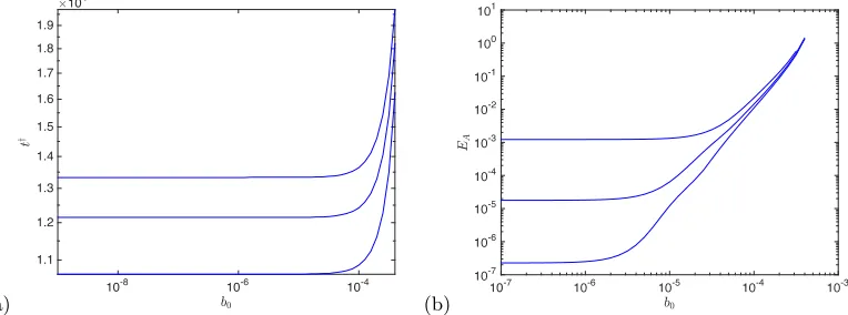
Figure 9. (a) The onset of flux expulsion t† as a function of initial field strength b0 using different thresholdsδ= 10−4, 10−3, and 10−2, reading down the curves. (b)
EAplotted against b0 at times 12T,T and 2T, reading down the curves.
3.2. Thresholds and scaling laws
We can summarise the results of the previous section as the presence of two thresholds. For a given flow field, the first is the thresholdb0=bcore(η) above which the Lorentz force
is so strong that flux expulsion does not occur and sot†,E
M andEAcannot be defined. Figure 9(a) showst†as measured numerically using several values ofδ(see below (3.1)). There is a sharp transition from the onset of flux expulsion at a time independent of initial field strength, to one that diverges rapidly withb0; at the same time the radiusr†
increases from 1.8 to around 2.2 (not shown). This sharp transition makes the threshold
b0=bcore(η) easy to measure, at least approximately.
The second, lower threshold isb0=bdynam(η) above which the field is sufficiently strong
(i.e. sufficientlydynamical) to modify the flow field and suppress diffusive decay. In this case the Lorentz force opposes differential rotation and results in solid body motion in a region near the origin. In terms of the flow field, this has the effect of turning offα1 in
[image:12.612.126.508.296.438.2]η
10-9 10-8 10-7 10-6
b0
10-7
10-6
10-5
10-4
[image:13.612.220.394.90.248.2]10-3
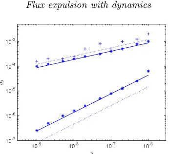
Figure 10.Thresholdsbcore(η) (upper dataset) andbdynam(η) (lower dataset) plotted against
η. In each case the data points come from a series of runs with varyingb0. The solid lines give the scalings η1/3 (upper) and η3/4 (lower). The dotted lines give the scalings from (5.4) and (5.7).
oscillations — see figure 8) at three times 12T, T and 2T and plot this against b0 in
figure 9(b). Where the curves cluster together on the right-hand side, the energy decays negligibly on theT time scale and we are in the dynamical core regime. Where the curves are spread out on the left-hand side, the field is so weak that the evolution is kinematic with a core decaying rapidly, that is, on theT time scale. The somewhat broad transition between these marks the thresholdbdynam(η), for this value ofη.
Neither of these thresholds is precisely defined, but in any case we are primarily interested simply in how they scale withη. We select a representative transitional field strengthbdynam to be the initial value of b0 for which log[EA(2T)/EA(T)] is half of its kinematic value. We estimated bdynam using a series of runs with 10 values of b0 per
decade on the logarithmic scale. For example in figure 9 we obtainbdynam = 7.9×10⁻⁶
forη= 10−7. Figure 10 shows b
dynam estimated this way, in the lower dataset, showing
good agreement with the scaling lawbdynam∼η3/4 (solid) from (5.5).
To estimate the thresholdbcore(η) for core formation we adopt two methods and these
are shown in the upper dataset in figure 10. The first is obtained by selecting the minimum field strengthb0for which the ratio EA(T)/EA(2T)<1.08 (asterisks), and this shows a good fit to the scaling lawbcore ∼η1/3 in (5.3), withbcore ≃4×10⁻⁴ at η = 10−7. For
another method, we chose the largestb0for which core formation, that is the existence of
a value oft†, was detected in our code (plus signs), givingb
core≃5×10⁻⁴atη = 10−7.
This also confirms the scaling law, albeit with more scatter. Note that alternatively we can use the scalings to rescale the vertical and the horizontal axes in figure 9(a,b) for a set of values ofηand so collapse the curves, which works well but which we do not show here.
Finally we comment on the numerical methods used. Equations (2.9–2.12) were written as a system of six first order PDEs for the real and imaginary parts of a, ∂ra, and v,
∂rv. This system was then passed to the NAG solver d03pef, which employs a Keller box method and integrates in time, withrlo6r6rhi forrlo= 0.05,rhi= 20 and up to
2×10⁴radial gridpoints in typical runs. At the inner and outer boundaries, the condition
of behaviour as rm was imposed on the vector potential, namely r∂
a magnetic core is formed, the outer boundary does not play a role, as discussed above, andrhi= 20 is sufficiently large (at least over the time scales shown here).
4. Calculation of the Lorentz force feedback
Our goal in this section is to derive the various scaling laws above, in particular those in figure 10. It is evident from figure 8 that the kinematic evolution is key, in that the dynamical curves typically follow the kinematic evolution, at least for a time. We consider the kinematic regime, corresponding to the limitb0→0 and a fixed flow field. We then
assess the feedback on the flow through the Lorentz force.
4.1. Flux expulsion: inner solution
We begin by recalling the classic flux expulsion calculation yielding (2.18) as an approximate outer solution to the equation (2.9). This gives a and j at radii where
α′(r) 6= 0 (fixed asη →0) and is valid for a general smooth profileα(r). However the approximation breaks down at the centre of the flow field whereα′(0) = 0 necessarily, and so another approximation, theinner solution, is needed there. Generally we assume that α(r) expands as (2.20) withα1 6= 0,†working in a kinematic regime, but we note
that in a dynamical regime the Lorentz force acts to suppress differential rotation given byα′(r). The kinematic theory is provided in BBG and is most easily set out by defining a length scaleL, time scaleT, their inverses, and a velocity scaleV by
k≡ L−1= (mα1/2η)1/4, p≡ T−1= (2ηmα1)1/2, V=L/T = (8η3mα1)1/4, (4.1)
and new variables by
τ=pt, ρ=kr. (4.2)
The exact solution to (2.9) may then be obtained with only the quadratic term retained in α(r) in (2.20), that isα≃α1r2 (where we also set α0 = 0 as solid body rotation is
irrelevant). The solution is
a=−12ib0k−mρmg e−if ρ
2
, (4.3)
j=−12ib0k2−mρmg[4i(m+ 1)f+ 4f2ρ2]e−if ρ
2
, (4.4)
wheref(τ) andg(τ) satisfy
∂τg=−2i(m+ 1)f g, ∂τf−1 =−2if2, (4.5) and so
f(τ) = (1 +i)−1tanh[(1 +i)τ], g(τ) ={cosh[(1 +i)τ]}−m−1. (4.6)
Now once a core has formed, for t > t†, undertaking the integrals in (3.1) gives straightforwardly
EM =π(m+ 1)!b20k−2m|g|2|f|2(−2fi)−m−2, (4.7)
EA=14π m!b20k−2m−2|g|2(−2fi)−m−1, (4.8)
withf =fr+ifi for brevity.
This is all exact if α(r) is given by only the leading terms, in α0 and α1 in (2.20).
The solution combines two different processes, with a crossover timeT defined in (4.1). Fort≪ T, the approximation captures a wave of flux expulsion, destruction ofa, in the locally quadratic angular velocity profile (2.20). In this regime, we have
f =τ−23iτ3+· · · , g≃1, −2fi ≃43τ
3, (4.9)
giving
EM ≃π(43)−m−2(m+ 1)!b20k−2mτ−3m−4=O(t−3m−4), (4.10)
EA≃ 14π(43)−m−1m!b20k−2m−2τ−3m−3=O(t−3m−3), (4.11)
and so algebraic behaviour of these quantities, with dependence as t−7 and t−6 in the
important casem= 1 of an initial uniform field, as seen in figure 4.
On the other hand for t ≫ T the solution describes an exponentially decaying core taking a Gaussian form near the origin, with
f ≃(1 +i)−1, g≃2m+1e−(m+1)(1+i)τ, −2f
i≃1, (4.12)
and
EM ≃22m+1π(m+ 1)!b02k−2me−2(m+1)τ, (4.13)
EA≃22mπ m!b20k−2m−2e−2(m+1)τ. (4.14)
Again this is confirmed by the results shown in figure 4 form= 1.
4.2. Lorentz force from the outer solution
We need to evaluate the Lorentz torqueGin (2.12) from the outer solution; however there is a cancellation at leading order when we substitute a and j from (2.18). To computeG we need to expand the flux expulsion solution systematically. This is most easily done by setting
a=−1
2ib0r
me−imαt+χ, (4.15)
where the complex functionχ, of space and time, gives the effect of flux expulsion. The current and Lorentz force are then
j=−1
2ib0r
m{m2α′2t2+im[α′′+ (2m+ 1)α′r−1+ 2α′χ′]t (4.16)
−[χ′′+χ′2+ (2m+ 1)χ′r−1]}e−imαt+χ,
G= 1
4mb 2
0r2m{2m[α′′+ (2m+ 1)α′r−1+α′(χ′+χ′∗)]t (4.17)
+i[(χ′′−χ′′∗) + (χ′2−χ′∗2) + (2m+ 1) (χ′−χ′∗)r−1]}eχ+χ∗
,
without approximation.
Now to calculateχ we introduceT =η1/3t as the time scale on which flux expulsion
occurs, and setχ=χ(r, T). The exact equation forχfollows from (2.9) and is
∂Tχ=−m2α′2T2−imη1/3[α′′+(2m+1)α′r−1+2α′χ′]T+η2/3[χ′′+χ′2+(2m+1)χ′r−1],
(4.18) where as usual the prime denotes anr-derivative at constantT (ort). A series approxi-mation forχcan now be developed, with expansion parameter η1/3≪1. Explicitly
with
χ0=−13m2α′2T3=−13m2ηα′2t3, (4.20)
χ1=−12im[α′′+ (2m+ 1)α′r−1]T2+154im3α′2α′′T5 (4.21)
=−12im[α′′+ (2m+ 1)α′r−1]η2/3t2+154im3η5/3α′2α′′t5. (4.22) To obtain the Lorentz torque at leading order (first line of terms inGin (4.17)) we need onlyχ0, which then gives
G≃1
2m 2b2
0r2m{[α′′+ (2m+ 1)α′r−1]t−43m
2ηα′2α′′t4}e−2 3m
2 ηα′2
t3
. (4.23)
Here we see that despite the initial quadratic growth with time t of the current j in (2.18), the Lorentz torqueGgrows only linearly via the first two terms (the latter term being small fort=O(1), η≪1). However at the time of flux expulsiont=O(η−1/3) all
the terms in Gin (4.23) are of the same order, and so all are important in computing the Lorentz force up to and during the destruction of field through flux expulsion.
4.3. Feedback through the Lorentz force: outer solution
We now discuss the effects of the Lorentz force on the flow: this features in the evolution of azimuthal velocityv,
∂tv=r−1G+ν(∆0v−r−2v), (4.24)
which in turn gives the equation for the angular velocity gradientα′,
∂tα′ = (r−2G)′+ν[r−1(∆0v−r−2v)]′. (4.25)
It is this key quantity we shall use. Our working hypothesis is that the Lorentz force has the effect of flattening the angular velocity at radiusrif the term (r−2G)′ evaluated kinematically and integrated over all time, is comparable or bigger thanα′at that radius. The threshold to consider is then when
α′(r)∼
Z ∞
0
[r−2G(r, t)]′dt. (4.26)
Bearing in mind that the right hand side is quadratic in b0 and we are interested in
thresholds in terms ofb0, we set the key function we need as
h(r) =−α′(r)−1b−2
0
Z ∞
0
[r−2G(r, t)]′dt. (4.27)
The minus sign here arises as in (4.25) it is the integral on the right hand side which is being compared withreducing the angular velocity gradient fromα′(r) at t= 0 to zero at large timest. We will take up the discussion of the physics in section 5, but for the moment just focus on calculatingh(r) for the outer solution and then the inner one.
First we takeGas given from (4.23) withm= 1 now (to avoid unnecessary complexity) and obtain
[r−2G]′= 1 2b
2
0[G0(r)t+G1(r)ηt4+G2(r)η2t7]e− 2 3ηα
′2 t3
, (4.28)
with
G0(r) =α′′′+3α′′r−1−3α′r−2, G1(r) =−4α′α′′(α′′+α′r−1)−43α′2α′′′, G2(r) = 169α′3α′′2.
(4.29) Finally we integrate (4.28) from time zero to infinity using integration by parts and by setting the constantc0 defined by
c0=
Z ∞
0
(see Olveret al.2010, section 9.12) to obtain
h(r) =−c1η−2/3α′−7/3[G0(r) +α′−2G1(r) +52α′−4G2(r)], c1≡2−5/332/3c0, (4.31)
or, with the formulae for theGj(r) in (4.29) we obtain
h(r) =c1η−2/3α′−7/3[13α′′′+α′′r−1+ 3α′r−2−49α′′2α′−1]. (4.32)
This (implausible-looking) expression is correct for any α(r). However note that when we approach the origin,α(r) expands as in (2.20) and then
h(r)≃c2η−2/3α−14/3r−
10/3, c
2≡223−4/3c0. (4.33)
This is valid in theoverlap region L ≪r≪1 where both inner and outer solutions are valid (referring to figure 3). Before using this, we proceed to look at the feedback in the inner solution.
4.4. Feedback through the Lorentz force: inner solution
Near the origin where the above formulation breaks down, we need to use the inner solution (4.1–4.6) instead, which yields
G=mb20|g|2k2−2mρ2m(f +f∗)[(m+ 1)−i(f−f∗)ρ2]e−i(f−f
∗)ρ2
(4.34)
and hence (withm= 1) we find
(r−2G)′= 2b20|g|2k3(f2−f∗2)[−3iρ−(f−f∗)ρ3]e−i(f−f
∗)ρ2
. (4.35)
Now to obtainh(r) in (4.27) we divide byb2
0and byα′= 2α1k−1ρand integrate over all
time. With the use of (4.1) we obtain
h(ρ) =V−2Z ∞
0
|g|2(f2−f∗2)[3i+ (f−f∗)ρ2]e−i(f−f∗)ρ2
dτ. (4.36)
We have taken the liberty of thinking of hnow as a function of ρ=kr and taken the integral over τ =pt. We cannot evaluate this analytically, except for large ρ when the approximation (4.9) is valid throughout the time range giving the leading contribution to the integral, with
h(ρ)≃c3V−2ρ−10/3, c3≡28/33−4/3c0. (4.37)
This is valid in the overlap region 1≪ρ≪ L−1and making use of the definitions ofp,k
andρin (4.1) we recover (4.33) as we must. More generally we can plotV2h(ρ) in (4.36)
againstρas in figure 11 to give a universal curve for the Lorentz feedback at the centre of a vortex with a general, smooth angular velocity profile (that is, withα16= 0).
5. Scaling laws and related information
We can use the results in the last section to make a number of predictions for scaling laws. We begin with crude estimates and then give more precise versions. Our aim is to evaluate the accumulated effect of the Lorentz force at a given radiusr in a kinematic regime and compare this withα′(r) at that radius. We use&and.to denote inequality up to a constant of order unity. Recall that we are comparing
α′(r) and
Z ∞
0
(a)
0 1 2 3 4 5
0 0.1 0.2 0.3 0.4 0.5 0.6 0.7 .8 .9 1 (b)
10-1 1 1
[image:18.612.122.508.90.244.2]1 1 2 1 -8 1 -6 1 -4 1 2 1 1 2 1 4
Figure 11.Plot ofV2h(ρ) (solid) given in (4.36) againstρwith (a) linear scales, (b) log–log scales. In (b) the approximation (4.37) is shown dashed.
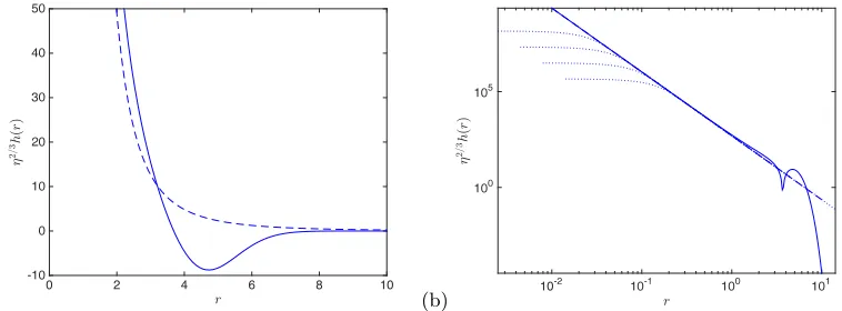
(a)
0 2 4 6 8 10
-1 1 3 4 5 (b) 10 1 -1 1 1 1 1 1 5
Figure 12.Plot ofη2/3h(r) (solid) given in (4.32) for the Gaussian vortex againstr with (a) linear scales, (b) log–log scales (taking the absolute value). In (a) the approximation (4.33) is shown dashed: it is also present in (b) but is somewhat overlapped with dotted curves showing
η2/3h(ρ) from (4.36) plotted againstrforη= 106 to 109, reading up the curves.
at a given radiusror range of radii. From the definition ofh(r) in (4.27) the integrated effect of the Lorentz force at radiusris sufficient to suppress the differential rotation if
b0∼h(r)−1/2. (5.2)
Also to fix ideas we ploth(r) in figure 12 for the Gaussian vortex (2.16) for a range ofη
values using the outer expansion (4.32) and the inner expansion (4.36).
Core formation threshold: first consider ifb0&bcore then at all radiirthe left-hand
side in (5.2) dominates. The Lorentz force (estimated by kinematic evolution) is strong enough to modify the flow field and suppress differential rotation and so flux expulsion. This represents the upper threshold for core formation. For greater fields, elastic forces dominate and prevent the onset of flux expulsion.
First of all, consider a basic estimate. The location where flux expulsion would com-mence is at the radiusr† of order unity where the differential rotation α′ is maximised, and it is here or nearby where the maximum inbcorewill be realised. At order one values
of radius we can use (4.32) which givesh(r) =O(η−2/3) and results in the threshold
bcore=O(η1/3), (5.3)
[image:18.612.130.509.280.420.2]To improve on this, it would make sense to minimise h(r) over all radii in view of (5.2) so as to maximise the field for flux expulsion to take place. However h(r) has a zero crossing, and we should note that the threshold for core formation is linked to Alfv´en wave generation, a process very far from the kinematic model we are using here. We do suggest instead a more precise estimate which brings in factors ofα1, taken by
substitutingr† in (4.33) to give
bcore(η) =c−21/2η1/3α
2/3
1 (r†)5/3. (5.4)
This is shown on figure 10 with good agreement, fortuitously good given that it is only correct up to a constant of unity.
Dynamical core threshold: now let us go to the other extreme. Ifb0.bdynamthen for
all radii the right-hand side of (5.2) dominates and the field will remain at leading order kinematic. A core will form through flux expulsion and will shrink to an exponentially decaying remnant at the origin following BBG. We thus need to look at where the maximum ofh(r) is realised. From (4.33) (see also figures 11, 12), from the point of view of the outer solution, we can increaseh(r) by reducing r. This represents the physical fact that the flow field is ‘naturally’ fairly flat near the origin, the field long-lived, and the Lorentz force required to flatten it completely becomes vanishing small. However this cannot continue indefinitely and we can argue this in two ways. First of all it is clear that this increasingh(r) in (4.33) (in the overlap region) must be cut off at radii
r∼ L=O(η1/4) in (4.1) where the overlap region ends and the inner solution really takes
over. Substituting this in (4.33) gives the maximum ofh(r) and the threshold estimated as
bdynam=O(η3/4) (5.5)
in agreement with figure 10 (lower dataset).
With more precision and elegance, we can move to the inner solution and figure 11(a) which shows thatV2his maximised at
c−42≡h(0) =
Z ∞
0
3i|g|2(f2−f∗2)dτ ≃0.91732 (5.6)
(obtained numerically) to give
bdynam =c4V =c4(8η3mα1)1/4, (5.7)
from (4.1). Thus we link the threshold field to the velocity scaleV based on the inner solution, which has the crucialη3/4dependence. This is plotted in figure 10 (lower dotted
line) showing good agreement up to a modest constant.
Onset of Lorentz force: finally suppose that b0 lies in the rangebdynam.b0 .bcore.
Then flux expulsion occurs at a radiusr†, a core is formed and a wave of flux expulsion spreads inwards. The Lorentz force however does become important at a radiusr∗(b0)
and timet∗(b0) given by
b0=h(r∗)−1/2, t∗= [13ηα′(r∗)2]−1/3. (5.8) These functions would depend on the original flow profile, but whenr∗ ≪ 1 then the approximation (4.33) in the overlap region comes into play (alsoα′(r
∗)≃2α1r∗) and we can estimate that
r∗≃c32/10b
3/5 0 η−1/5α
−2/5
1 t∗≃c5η−1/5b−02/5α −2/5
1 , c5= 2−2/331/3c−21/5. (5.9)
For example for η = 10−7 and b
agreement with figure 8.Note that at the lower and upper limits of the range bdynam .
b0.bcore, the core size is of orderLin (4.1) andr†, respectively.
6. Discussion
We have studied some of the effects of dynamical feedback on flux expulsion using a quasi-linear model, using both numerical simulation and theory based on the kinematic picture. We have identified two thresholds: returning to our original dimensional formulation before (2.15) and measuring magnetic field in velocity units,the first threshold isbcore∼
U R−m1/3 below which flux expulsion still operates, cutting field lines at the radiusr†and leaving a magnetic core within. The second is bdynam ∼U Rm−3/4 below which the field evolves as in the kinematic regime. Between the two thresholds a magnetic core is formed in which the flow field near the origin is modified to be solid body rotation at leading order, so halting the diffusive decay of the core.In the range betweenbcore and bdynam the core radius scales asL(b0/U)3/5R1m/5.†
In each case diffusive processes are key and the results depend sensitively on the magnetic diffusivity — only the cutting of fields lines by diffusion can halt the increase of Lorentz force as the field reduces in scale. With this in mind, we have made careful estimates based on the kinematic solutions, inner and outer, and we note that cruder arguments could easily lead to incorrect conclusions. For example, although the magnetic field grows linearly with time, the Lorentz force term also grows linearly in (4.23) and not quadratically as might be suggested by a simplistic estimate b· ∇b ∼ b2/L, L being the scale of the eddy, this overestimating the variation ofbalong field lines. Even worse would be to estimate the Lorentz force as jb = O(t3). Likewise in (4.26) it is
necessary to calculate the effect ofGintegrated from time zero up to the time when flux expulsion occurs (similar remarks apply in the kinematic regime, as discussed in Moffatt & Kamkar (1983)). It is also important to look at the effect on the differential rotation, not the velocity or angular velocity. Finally to pick up the lower thresholdbdynam the
scaling structure of the inner solution from BBG is needed, in particular relating the field magnitude toV =O(U R−m3/4). We also note that any replacement of the true magnetic diffusion term involving the Laplacian, by some hyperdiffusion or similar cut-off would change these scaling laws. Any use of hyperdiffusion in the induction equation must be treated with caution: although the change may have a minor impact on small-scale fields at any moment, here it would have a significant impact on the large-scale, long-time evolution.
Future directions of research could include generalising the geometry, for example to an axisymmetric eddy localised in three dimensions, and a magnetic field with initially an arbitrary orientation with respect to the eddy. It would also be interesting to study other regimes of the Reynolds numbers. We have taken onlyRe ≫Rm ≫ 1, although we expect our results to have wider applicability, we think at least up toRe∼Rm. The ordering Re ≫ Rm ≫ 1 is relevant in typical astrophysical and geophysical contexts, and so the modelling could be broadly relevant to the formation of magnetic fields in the early life of some astrophysical objects, for example the relict magnetic field likely to lie in the radiative zone of the Sun (e.g. Mestel & Weiss 1986). At least it indicates the importance of taking into account small scale reconnection processes that depend on molecular transport coefficients, even in the formation of large-scale fields, this also
being the point originally stressed by Vainshtein & Cattaneo (1992) in the context of dynamo theory.
A related problem would be to consider an initial two-dimensional turbulent flow containing eddies or vortices, on a range of length scales: which of these would develop dynamical magnetic cores, and what would be their distribution? For what field threshold would the evolution over all length scales be entirely kinematic? Finally, it would be valuable to study dynamical flux expulsion numerically by means of full simulations in unbounded geometry and explore the limitations of the quasi-linear approximation as set out here. Simulations withRe≫Rm≫1 can be undertaken efficiently using contour– spectral methods (Dritschel & Tobias 2012) while regimes withRe∼Rm≫1 would be best simulated with standard pseudo-spectral codes.
Acknowledgements
This paper is dedicated to Konrad Bajer (Warsaw University), an inspiring colleague who contributed greatly to the field of fluid mechanics and who sadly passed away in August 2014. We thank Keith Moffatt, Andrew Soward and Nigel Weiss for useful discussions and the referees for helpful comments leading to improvements in the manuscript.
RE FERE N CE S
Bajer, K.1998 Flux expulsion by a point vortex.Eur. J. Mech. B/Fluids 17, 653–664.
Bajer, K., Bassom, A.P. & Gilbert, A.D. 2001 Accelerated diffusion in the centre of a vortex.J. Fluid Mech.437, 395–411. Referred to as BBG in the text.
Bassom, A.P. & Gilbert, A.D. 1997 Nonlinear equilibration of a dynamo in a smooth helical flow.J. Fluid Mech.343, 375–406.
Bernoff, A.J. & Lingevitch, J.F. 1994 Rapid relaxation of an axisymmetric vortex.Phys. Fluids 6, 3717–3723.
Cattaneo, F. & Vainshtein, S.I. 1991 Suppression of turbulent transport by weak magnetic field.
Astrophys. J.376, L21–24.
Cattaneo, F. 1994 On the effects of a weak magnetic field on turbulent transport.Astrophys. J. 434, 200–205.
Dritschel, D.G. & McIntyre, M.E. 2008 Multiple jets as PV staircases: the Phillips effect and the resilience of eddy-transport barriers.J. Atmos. Sci.65, 855–874.
Dritschel, D.G. & Tobias, S.M. 2012 Two-dimensional magnetohydrodynamic turbulence in the small magnetic Prandtl number limit.J. Fluid Mech.703, 85–98.
Galloway, D.J., Proctor, M.R.E. & Weiss, N.O. 1978 Magnetic flux ropes and convection. J. Fluid Mech.87, 243–261.
Julien, K., Rubio, A.M., Grooms, I. & Knobloch, E. 2012 Statistical and physical balances in low Rossby number Rayleigh–B´enard convection.Geophys. Astrophys. Fluid Dyn. 106,
392–428.
Keating, S.R. & Diamond, P.H. 2008 Turbulent resistivity in wavy two-dimensional magnetohydrodynamic turbulence.J. Fluid Mech.595, 173–202.
Keating, S.R., Silvers, L.J. & Diamond, P.H. 2008 On cross-phase and the quenching of the turbulent diffusion of magnetic fields in two dimensions.Astrophys. J.678, L137–140.
Kim, E.-J. 2006 Consistent theory of turbulent transport in two dimensional magnetohydrody-namics.Phys. Rev. Lett.96, 084504.
Mestel, L. & Weiss, N.O. 1986 Magnetic fields and non-uniform rotation in stellar radiative zonesMNRAS 226, 123–135.
Moffatt, H. K., 1978 Magnetic field generation in electrically conducting fluids. Cambridge University Press.
Olver, F.J.W., Lozier, D.W., Boisvert, R.F. & Clark, C.W. 2010NIST handbook of mathematical functions.Cambridge University Press.
Parker, R.L. 1966 Reconnection of lines of force in rotating spheres and cylinders.Proc. R. Soc. Lond. A291, 60–72.
Rhines, P.B. & Young, W.R. 1983 How rapidly is a passive scalar mixed within closed streamlines?J. Fluid Mech.133, 13–145.
Srinivasan, K. & Young, W.R. 2012 Zonostrophic instability.J. Atmos. Sci.69, 1633–1656. Taylor, J.B. 1963 The magnetohydrodynamics of a rotating fluid and the Earth’s dynamo
problem.Proc. R. Soc. A9, 274–283.
Tobias, S.M. & Cattaneo, F. 2008 Limited role of spectra in dynamo theory: coherent versus random dynamosPhys. Rev. Lett.101, 125003
Tobias, S.M., Dagon, K.& Marston, J.B. 2011 Astrophysical fluid dynamics via direct statistical simulation.Astrophys. J.727, 127.
Vainshtein, S.I. & Cattaneo, F. 1992 Nonlinear restrictions on dynamo actionAstrophys. J.393,
165–171.
Weiss, N.O. 1966 The expulsion of magnetic flux by eddiesProc. R. Soc. Lond. A293, 310–328.