Negative-free approximation of probability density function for nonlinear projection filter

This is a repository copy of

Negative-free approximation of probability density function for

nonlinear projection filter

.

White Rose Research Online URL for this paper:

http://eprints.whiterose.ac.uk/103369/

Version: Accepted Version

Proceedings Paper:

Kim, J orcid.org/0000-0002-3456-6614 and Richardson, R (2016) Negative-free

approximation of probability density function for nonlinear projection filter. In: 2016 IEEE

55th Conference on Decision and Control (CDC). 55th IEEE Conference on Decision and

Control, 12-14 Dec 2016, Las Vegas, Nevada, United States. IEEE , pp. 3738-3743. ISBN

978-1-5090-1837-6

https://doi.org/10.1109/CDC.2016.7798832

© 2016, IEEE. This is an author produced version of a paper published in 2016 IEEE 55th

Conference on Decision and Control (CDC). Personal use of this material is permitted.

Permission from IEEE must be obtained for all other users, including reprinting/

republishing this material for advertising or promotional purposes, creating new collective

works for resale or redistribution to servers or lists, or reuse of any copyrighted

components of this work in other works. Uploaded in accordance with the publisher’s

self-archiving policy.

[email protected] https://eprints.whiterose.ac.uk/

Reuse

Unless indicated otherwise, fulltext items are protected by copyright with all rights reserved. The copyright exception in section 29 of the Copyright, Designs and Patents Act 1988 allows the making of a single copy solely for the purpose of non-commercial research or private study within the limits of fair dealing. The publisher or other rights-holder may allow further reproduction and re-use of this version - refer to the White Rose Research Online record for this item. Where records identify the publisher as the copyright holder, users can verify any specific terms of use on the publisher’s website.

Takedown

If you consider content in White Rose Research Online to be in breach of UK law, please notify us by

Negative-free approximation of probability density function for

nonlinear projection filter*

Jongrae Kim

, and Robert Richardson

Abstract— Several approaches have been developed to

esti-mate probability density function (pdf). The pdf has two im-portant properties: the integration of pdf over whole sampling space is equal to 1 and the value of pdf in the sampling space is greater than or equal to zero. The first constraint can be easily achieved by the normalisation. On the other hand, it is very hard to impose the non-negativeness in the sampling space. In the pdf estimation, some areas in the sampling space might have negative pdf values. It produces unreasonable moment values such as negative probability or variance. A transformation to guarantee the negative-free pdf over a chosen sampling space is presented and it is applied to the nonlinear projection filter. The filter approximates the pdf to solve nonlinear estimation problems. For simplicity, one-dimensional nonlinear system is used as an example to show the derivations and it can be readily generalised for higher dimensional systems. The efficiency of the proposed method is demonstrated by numerical simulations. The simulations also show that to achieve the same level of approximation error in the filter the required number of basis functions with the transformation is a lot smaller compared to the ones without transformation. This will be hugely benefited when the filter is used for high dimensional systems, which requires significantly less computational cost.

I. INTRODUCTION

Nonlinear estimation has been one of the most studied topics in control theory in the last half century since the success of Kalman filter [1] in the Apollo mission [2]. The orbit estimation problem in the Apollo mission is nonlinear and the initial success of the Kalman filter relied on the assumption of the reasonable error bounds in the perturbed state, which can be approximated by a linear dynamics, and it is called the extended Kalman filter. The extended Kalman filter has been applied to many dynamical systems including the attitude estimation problem for satellite [3], the target tracking problem such asα-β filter [4] andα-β-γ filter [5], a traffic management [6], and plethora of many other examples. It was, however, quickly realised that the limitation of the extended Kalman filter or linearised approach to nonlinear estimation, in general. If the initial guess is not close enough to the region, where the linearisation is valid, then the estimated state could diverge. In order to resolve the issues, unscented Kalman filter is proposed [7]. Using a nonlinear transformation, the unscented Kalman filter improves the linearisation accuracy up to the 3rd-order in Taylor series

*This research is supported by EPSRC Research Grant, EP/N010523/1, Balancing the impact of city infrastructure engineering on natural systems using robots.

1_{J.Kim and R.Richardson are with Institute of Design, Robotics &}

Optimisation, School of Mechanical Engineering University of Leeds, Leeds LS2 9JT, UK.{menjkim,r.c.richardson}@leeds.ac.uk

expansion [8]. Several examples of the unscented Kalman filter applications can be found in [9]–[11].

True nonlinear estimation can be obtained by solving the Fokker-Plank equation [12], which governs the propagation of the underlying joint probability density function (pdf) for a given nonlinear system, while the propagation is updated using the Bayes’ rule whenever a measurement is available. The particle filter is based on these mechanisms [13], where the required multi-dimensional integration is performed by the Monte-Carlo sampling method. One of the main issues in the particle filter is that the sampling points are quickly concentrated in a few sampling spaces and the re-sampling methods are developed to rectify the problem, which does not solve another problem with highly variable cases [14].

The nonlinear projection filter presented in [15] solves the Fokker-Planck equation in a different way compared to the particle filter. The solution of the Fokker-Planck equation is assumed to be a linear combination of a set of orthogonal basis functions. The dynamics of the time-varying variables to combine the basis function is obtained and used for propagating the time-varying variables; and they are updated based on the Bayes’ rule when a measurement is available. It has been applied to a target tracking problem [16]–[18] and there are a few variations of the filter via combining with particle samplings [19], [20] or performing the multi-dimensional integration combining with multiple sensor measurements [21].

As it is emphasised, however, in [21], the approximated pdf might not satisfy all requirements for any pdf to content. The integration of pdf over whole sampling space must be equal to 1. This condition can be easily met for the filter by normalising the estimated pdf every propagation and/or up-date step. On the other hand, the non-negativeness condition, which requires the pdf greater than equal to zero in every point in the sampling space, is the one that hard to comply with. It is not easy to impose the non-negativeness during the propagation and the update steps. The negativeness issue will not be resolved via simply increasing the number of basis functions. This is a similar problem in the Fourier transform called the Gibbs phenomena [22].

proposed using a log function. This is partially inspired by the method presented in [23].

This paper organises as follows: firstly, the summary of the nonlinear projection filter is presented; secondly, a transformation for prohibiting the negativeness of pdf is presented along with the detail derivations of the filter for a one-dimensional nonlinear system, where we highlight that for many cases analytic expression can be obtained for a general type of multi-dimensional nonlinear systems. Thirdly, numerical simulations are performed to show the effectiveness of the proposed transformation and to compare the results with the ones without the transformation. Finally, the conclusions are presented.

II. NONLINEAR PROJECTION FILTER

One of the standard forms of nonlinear stochastic system is given by

dx=f(x)dt+G(x)dβ (1)

for t_≥t0, where x is an n-dimensional state, β(t) is a b -dimensional Brownian motion, E(β βT) =Q(t)dt,E(·)is the expectation, (·)T _{is the transpose, f(·) is an n-dimensional}

nonlinear function, and G(·) is an n_×b matrix. The mea-surement is given by

y_k=h(xk) +v_k (2)

for k_≥1, where yk is an m-dimensional real vector, vk

is a white noise whose covariance is Rk, and h(·) is the

m-dimensional measurement function. It is assumed that

β(t)andvk are not correlated.

The conditional probability density function can be written as follows:

p(t,x_|Yk) = p(t,x,Yk)

p(Yk) ,

whereY_k is the collection of all measurement up to t_k≤t. The time evolution of the conditional pdf is governed by the Fokker-Planck equation:

∂p ∂t =−

n

∑

∂(p fi)

∂xi +1

2

n

∑

n

∑

∂2h_{p GQG}T i,j

i

∂xi∂xj

(3)

wherexi and fi are the i-th element of x andf(x),

respec-tively, (GQGT)i,j is the i-th row and j-th column element

of the matrix, GQGT, and the initial condition is given by

p(t0,x). Once the conditional pdf is obtained, any moment can be calculated as follows:

Exℓ1

1x ℓ2

2 . . .x ℓn

n

=

Z

Ω

xℓ1

1x ℓ2

2 . . .x ℓn

n

p(x,t_|Yk)dx,

where Ω is a closed bounded subset of Rn _{and ℓi for}

i=1,2, . . . ,n is a real number.

The nonlinear projection filter is derived by assuming the pdf as a linear combination of basis functions as follows:

p(t,x_|Yk)≈pN(t,x|Yk) = N

∑

cℓ(t)φℓ(x), (4)

where the basis functions are orthogonal

Z

Ωφi(x)φj(x)

dx= (

1 for i=j,

0 for i₆=j (5)

fori,j=1,2,3, . . . ,N₋1,N.

Propagation: Substituting (4) into (3), projecting onto φq

and integrating over Ω provide the following differential equation forc(t):

˙

c(t) = (A1+A2)c(t), (6)

where (˙) is the derivative by time, the initial condition is equal to

c(t0) =

Z

Ω

p(t0,x)φ(x)dx,

φ(x) = [φ1(x), φ2(x), . . . , φN(x)]T, and theith-row and j th-column element ofA1or A2is given by

[A1]i,j=− n

∑

Z

Ω

∂[φjfk]

∂x_k φidx,

[A2]i,j=

1 2

n

∑

n

∑

Z

Ω

∂2h_φ

j GQGT_k,ℓ i

∂xk∂xℓ φi

dx.

Update: The conditional probability density function is updated by the Bayes’ rule at the measurement available from a sensor [13]. Substituting (4) into the Bayes’ rule, the update equation is obtained as follows:

c(t_k+) =η

Y(yk)c(t_k−)

(8)

wheret_k+andt_k−indicate after and before thek-th measure-ment are considered,

Y(yk) =

Z

Ω

p(yk|x)φ φTdx

and η is the normalising constant. The full details on the nonlinear projection filter derivation can be found in [15].

III. NEGATIVE-FREE PDF APPROXIMATION

In the nonlinear projection filter with the basis function ap-proach, the main issue is the negativeness of the probability in some places of the sampling space. To reduce the size of the negative probability area, the number of basis functions must increase quite significantly. The computational cost increases exponentially as the number of basis functions increases. This would be the one of main obstacles in the applications of the filter to some reasonable size systems

For simplicity, all derivations from now on are based on the following nonlinear system [15]:

dx=sin(x)dt+dβ (9)

with a measurement equation equal to

yk=xk+vk (10)

where the variance of the process noise,β(t), is equal toq, and the variance of the measurement noise,vk, is equal to

A. Transformation

Defineρ(t,x_|Yk)using the joint pdf, p(t,x_|Yk)

ρ(t,x_|Yk) =ln[p(t,x_|Yk) +ε] (11)

whereε is a small positive real number in order to prevent the log-function becoming the negative infinity or a large negative value for p(t,x_|Yk) to approach to zero arbitrary close. As the domain of x, i.e., Ω, less likely includes the regions where the joint pdf is exactly equal to zero, the following assumption is introduced without imposing any strong restriction:

Assumption 3.1: Ωis chosen such thatδ in the following inequality is close to zero but not exactly zero.

0<δ_≤min

t≥0 x_∈Ω

[p(t,x_|Yk)] (12)

Hence,εcan be set to very close to zero and a lower bound of ρ(t,x_|Yk)is given by

−∞<ln(δ+ε)≤ρ(t,x_|Yk) (13) andρ(t,x)can be negative unlikep(t,x)≥0 for allt_∈[0,∞)

andx_∈Ω. The inverse transformation is simply

p(t,x_|Yk) =eρ(t,x|Yk)_{−ε (14)}

In practice,εcan be chosen to be very close to zero allowed by the given numerical precision.

B. Propagation

Take the time derivative of the inverse transformation

d p(t,x_|Yk)

dt =e

ρ(t,x|Yk)dρ(t,x|Yk)

dt (15)

Substitute (14) and (15) into the Fokker-Planck equation, (3),

eρdρ dt =−e

ρ

sin(x)ρ′+(eρ₋ε)cos(x)+q

2

eρ(ρ′)2+eρρ′′

where(·)′=d(·)/dxand(·)′′=d2(·)/dx2. Divide both sides byeρ, which is greater thanε,

˙

ρ=−sin(x)ρ′+e

ρ_−ε

eρ cos(x) +

q

2

(ρ′)2_+ρ′′

(16)

In the nonlinear projection filter [15], it is proposed that the joint pdf is approximated by (4). The approximation uses a set of basis functions and it does not force the approximated values at all x in Ω be non-negative. On the other hand, as ρ(t,x_|Yk) can be positive or negative, it is natural to approximateρ(t,x_|Yk)instead of p(t,x_|Yk)by a set of basis functions without concerning to impose non-negativeness. Let

ρ(t,x) =cT(t)φ(x) (17)

and substitute the approximation into (16)

˙

cTφ=−sin(x) cTφ′ +e

cTφ_−ε

ecT_φ cos(x)

+q

2

(cTφ′)2+cTφ′′

(18)

where theN-number of cosine-basis functions are chosen

φi(x) =  



1/√∆_x for i=1,

r

2

∆_xcos[κi(s−ax)] for 2≤i≤N

(19)

∆_x is equal tobx−ax, ax is the lower bound of x,bx is the

upper bound ofx, i.e.,x_∈[ax,bx]andκi= [(i−1)π]/∆x for

i=1,2, . . . ,N. The basis functions satisfy the orthogonality condition.

Proposition 3.2: The basis functions are satisfied

φ′(x) =−Kψ(x) (20a)

φ′′(x) =−K2φ(x) (20b)

where

K=diagκ1 κ2 . . . κN

, (21a)

ψ(x) = r

2

∆_x 

     

0 sin[κ2(s−ax)] sin[κ3(s−ax)]

.. . sin[κN(s−ax)]



     

, (21b)

Proof: The proof is straightforward and omitted. The full

derivations can be found in [18].

Using the proposition 3.2, (18) becomes

˙

cTφ=−sin(x) cTKψ +e

cTφ_−ε

ecT_φ cos(x)

+q

2

(cTKψ)2−cTK2φ

(22)

Multiplyφ both sides and integrate overΩ

˙

c=−

Z

Ωsin(x) ψ T_Kφ

dx c+

Z

Ω

ecTφ₋ε

ecT_φ cos(x)φdx

+q

2

Z

Ω(c

T_Kψ)2_φdx

−q

2K 2_c

(23)

Re-arrange it

˙

c=− Z

Ωsin(x) ψ T_Kφ

dx+q

2K 2

c

+

Z

Ω

ecTφ₋ε

ecT_φ cos(x)φdx+

q

2

Z

Ω(c

T_Kψ)2_φdx (24)

Some of the integrals in the right hand side of (24) have analytic expression. The first row of the first integral is zero,

Z

Ωsin(

x) ψT_Kφ dx

1j

=0 (25)

for j=1,2, . . . ,N. The diagonal terms are given by

Z

Ωsin(x) ψ T_Kφ

dx

ii

=2(i−1)

2_π2_{[sin(b)−sin(a)]}

∆x[∆2

x−4π2(i−1)2]

(26)

fori=2,3, . . . ,N. Note that∆_xmust not be equal to 2π(i₋1)

Assumption 3.3: ∆_xis not equal toℓπfor allℓinN_{, where} N_{is the set of natural number.}

The assumption is not strong asΩcan be always adjusted so that the boundary length is not equal toℓπ. The non-diagonal terms have an analytic expression but the expression is too long and omitted.

Consider the magnitude difference between the second term in (24) and the one with ε equal to zero.

∆=

Z

Ω

ecTφ₋ε

ecT_φ cos(x)φdx−

Z

Ωcos(

x)φdx _∞

= ε

ecT_φ

Z

Ωcos(x)φdx _∞≤

ε ecT_φ ≤

ε

δ+ε (27)

where k · k∞ is the infinity norm. Set ε equal to γ-times

smaller than δ, where 0≤γ≪1, the error is bounded by the following inequality:

∆_≤ ε δ+ε =

γδ δ+γδ =

γ

1+γ ≪1 (28)

whereε is very small by Assumption 3.1. Given the choice of ε=γδ, the second integration term is approximated by

Z

Ω

ecTφ₋ε

ecT_φ cos(x)φdx≈

Z

Ωcos(

x)φdx (29)

and the integral with the approximation has an analytic expression. Define b=R

Ωcos(x)φdxand it becomes

b= 

              

sin(bx)−sin(ax)

√_∆

x

√

2 ∆3_x/2

sin(bx)(−1)2+1_−sin(ax) ∆2

x−(2−1)2π2

√

2 ∆3x/2sin(bx)(−1)3+1−sin(ax)

∆2

x−(3−1)2π2

.. .

√

2 ∆3x/2sin(bx)(−1)N+1−sin(ax)

∆2

x−(N−1)2π2



              

(30)

The k-th element of the last integration term in the right hand side of (24) can be reformulated as follows:

Z

Ω(c

T_Kψ)2_φdx

k =

Z

Ω(c T_Kψ)2_φ

kdx

=

Z

Ω N

∑

N

∑

cicjκiκjψiψjφkdx

= Z

Ω(ψ

T_⊗ψT_)φ kdx

(K_⊗K)(c⊗c)

=sT_k(K_⊗K)(c⊗c) (31)

wheresT_k is equal to the integration of(ψT_⊗ψT_)φ

koverΩ,

and its size isN2_×1. Define

S=

s1 s2 . . . sNT (32)

whose size is N_×N2. Note that S has most of the terms equal to zero. The last integration term of (24) is given by

Z

Ω(c

T_Kψ)2_{φdx=S(K⊗K)(c⊗c) (33)}

Considerℓ-th element ofsk

(sk)_ℓ=

Z

Ωψiψjφk

dx (34)

whereℓ= (i₋1)N+j. It is trivial that all integrations with

ψ1 is equal to zero asψ1=0. Also, it can be easily shown that all integrations in the following index set are equal to zero:

{(i,j,k)|i₆=j+k₋1 or j₆=i+k₋1 ork₆=i+j₋1} (35)

for i, j,k are in [1,N]. For the case of either i= j+k₋1 or j=i+k₋1, (sk)ℓ is equal to 1/√2∆_x. For the case of

k=i+j₋1, (sk)ℓ is equal to−1/√2∆x.

Finally, the differential equation ofc(t)can be written in a compact form as follows:

˙

c=fc(c) =−Ac+b+q

2[S(K⊗K)] (c⊗c) (36)

where

A=

Z

Ωsin(

x) ψT_Kφ dx+q

2K

2 ₍₃₇₎

Note thatSand(K_⊗K)are sparse and can be obtained for large size N without requiring long computation and large memory size. For each sampling time, the above differential equation is used to propagatec(t)fromt=tk tot=tk+1 as follows:

c(t_k+1) =Φ[t_k+1,t_k,c(t_k)] (38)

wheretk+1=tk+∆tk,Φ(·)is the transition function. In the

original propagation with p(t,x_|Yk) =cT(t)φ(x) in [15], the differential equation forc(t)is linear and the transition func-tion can be obtained off-line. The propagafunc-tion equafunc-tion with

ρ(t,x_|Yk), (36) is nonlinear. Hence, the transition function has to be calculated on-line. The following algorithm is proposed to propagatec(tk):

Algorithm 3.4: c(t_k)propagation toc(t_k+1)

1) Selectnp, a positive integer, and set∆t=∆tk/np,ℓ=0,

andcℓ=c(tk)

2) Calculate

cnew=cℓ+∆t fc[cℓ] (39)

3) Increaseℓ by one, i.e.,ℓ←ℓ+1 4) Setcℓ=cnew

5) If ℓ=np, setc(tk+1) =cℓ and stop. Otherwise, go to

(a)N=16

0 2 4 6 8 10

−7 −6 −5 −4 −3 −2 −1 0 1 2

time [s]

x

(t)

0 0.1 0.2 0.3 0.4 0.5 0.6 0.7 0.8 0.9 1 true

measurement

(b)N=64

0 2 4 6 8 10

−7 −6 −5 −4 −3 −2 −1 0 1 2

time [s]

x

(t)

0.1 0.2 0.3 0.4 0.5 0.6 0.7 0.8 0.9 1 true

measurement

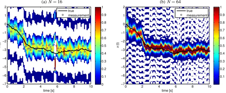
Fig. 1. Without the transformation: the regions in white colour are the space where the pdf is negative. The heat-map indicates the time-history of the pdf over the sampling space. The true state is shown by the black solid line and the measurements are depicted by the hollow circles.

C. Update

The conditional probability density function is updated using the current measurement by Bayes’ rule [13]:

p(t_k+,x_|Yk) =ηp(yk|x) p(tk−,x|Yk−1) (40)

whereη is the normalising constant to be determined, and

p(yk|x) is the sensor model. To determine the normalising

constant,η, integrate (40) over the sampling space,Ω,

Z

Ω

p(t_k+,x_|Yk)dx=η

Z

Ω

p(yk|x) p(t_k−,x|Yk₋1)dx (41)

where the left hand side is equal to 1 as it is the total probability. Hence,

η= Z

Ωp(yk|x) p(t −

k,x|Yk−1)dx

−1

(42)

Substituting the inverse transformation, (14), into, (42), and

η is calculated as

η= Z

Ω

p(y_k|x) hecT(tk)φ(x)_−ε

i dx

−1

(43)

This integral must be performed on real-time and the Monte-Carlo integration method was proposed in [21]. Sample the random points based on the sensor model provides an efficient integration performance, which reduces the required sampling points significantly. See [21] for details.

Substituting the pdf approximation with the transformation into (40)

eρ(tk+1,x|Yk)_−ε=ηp(y

k|x)p(tk−,x|Yk−1) (44)

Take log both sides

ρ(tk+1,x|Yk) =log

ηp(yk|x)p(tk−,x|Yk−1) +ε

(45)

and replaceρ(t_k+1)by the approximation

cT(tk+1)φ(x) =log

ηp(yk|x)p(tk−,x|Yk−1) +ε

(46)

Finally, multiplyφT_{(x) both sides and integrate overΩ}

c(t_k+1) =

Z

Ωlog

ηp(yk|x)p(t_k−,x|Yk₋1) +εφ(x)dx, (47)

which provides the update equation. Again, this integration must be performed on real-time and the efficient sampling could be implemented based on the a priori joint pdf,

p(t_k−,x_|Yk−1).

IV. SIMULATION

The variances of the noises in the system and the sensor are set toq=0.5 andr=0.5, respectively. The measurement is taken every 0.1s. The state variable, x, is in the range of

[−2.2π,2.2π]and the initial state is equal to zero. The sensor is assumed to have the following noise model:

p(yk|x) =

1

√

2πr e

−(yk−x)2/(2r) ₍₄₈₎

To compare the performance, the same measurement set is used for the filter without the transformation and the one with the transformation. ε for the transformation is set to 10−300.

Figure 1 shows the results without the transformation for the number of basis functions equal to 16 or 64. Both cases have large areas with the negative pdf, which is depicted by the white colour. ForN=16, around the time equal to 5.8s, the negative region even appears across the true value. For

N=64 the negativeness still exist in the wide areas. In order to reduce the negative region significantly, N must be very large. This causes serious issues in applying the filter for higher dimensional systems as the number of basis function increases withNn_{, wherenis the dimension of state. Hence,}

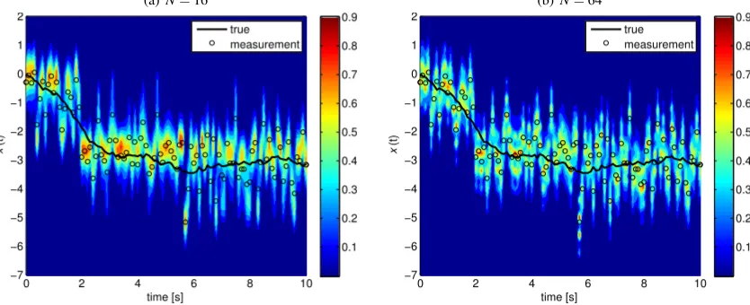
it is important to keep N small. The filtering results for the same data set with the transformation are shown in Figure 2. As shown in the figure, they do not have any negative region by the definition and the quality of estimation is not distinguishable in the results for N =16 and N =64. Hence, the number of basis functions could be kept lower, for example, as small asN=5 in this case (simulation result is not shown).

V. CONCLUSIONS

(a) N=16

0 2 4 6 8 10

−7 −6 −5 −4 −3 −2 −1 0 1 2

time [s]

x

(t)

0.1 0.2 0.3 0.4 0.5 0.6 0.7 0.8 0.9 true

measurement

(b)N=64

0 2 4 6 8 10

−7 −6 −5 −4 −3 −2 −1 0 1 2

time [s]

x

(t)

0.1 0.2 0.3 0.4 0.5 0.6 0.7 0.8 0.9 true

measurement

Fig. 2. With the transformation: the pdf does not have negative values by the definition. The heat-map indicates the time-history of the pdf over the sampling space. The true state is shown by the black solid line and the measurements are depicted by the hollow circles.

approximation is used to derive the nonlinear projection filter, where the joint probability density function is estimated. It is shown that some analytic expressions can be derived with the set of cosine basis functions and this could be applicable for various types of nonlinear functions. In addition, the required number of basis functions could be reduced significantly and it would enable to apply the filter to higher-dimensional systems. The effectiveness of the proposed method is demon-strated by some numerical simulations.

ACKNOWLEDGEMENT

This research is supported by EPSRC Research Grant, EP/N010523/1, Balancing the impact of city infrastructure engineering on natural systems using robots.

REFERENCES

[1] R. E. Kalman, “A New Approach to Linear Filtering and Prediction Problems,”Transactions of the ASME Journal of Basic Engineering, no. 82 (Series D), pp. 35–45, 1960.

[2] M. S. Grewal and A. P. Andrews, “Applications of Kalman Filtering in Aerospace 1960 to the Present [Historical Perspectives],” Control Systems, IEEE, vol. 30, pp. 69–78, June 2010.

[3] E. J. Lefferts, F. L. Markley, and M. D. Shuster, “Kalman filtering for spacecraft attitude estimation,”Journal of Guidance, Control, and Dynamics, vol. 5, pp. 417–429, September-October 1982.

[4] S. Rogers, “Alpha-beta filter with correlated measurement noise,” Aerospace and Electronic Systems, IEEE Transactions on, vol. AES-23, pp. 592–594, July 1987.

[5] J. Gray and W. Murray, “A derivation of an analytic expression for the tracking index for the alpha-beta-gamma filter,” Aerospace and Electronic Systems, IEEE Transactions on, vol. 29, pp. 1064–1065, July 1993.

[6] C. Antoniou, M. Ben-Akiva, and H. N. Koutsopoulos, “Nonlinear kalman filtering algorithms for on-line calibration of dynamic traffic assignment models,”IEEE Transactions on Intelligent Transportation Systems, vol. 8, pp. 661–670, Dec 2007.

[7] S. J. Julier and J. K. Uhlmann, “Unscented filtering and nonlinear estimation,”Proceedings of the IEEE, vol. 92, pp. 401–422, Mar. 2004. [8] E. Wan and R. Van Der Merwe, “The unscented Kalman filter for nonlinear estimation,” in Adaptive Systems for Signal Processing, Communications, and Control Symposium 2000. AS-SPCC. The IEEE 2000, pp. 153–158, IEEE, Aug. 2000.

[9] J. L. Crassidis and F. L. Markley, “Unscented filtering for spacecraft attitude estimation,” Journal of Guidance, Control, and Dynamics, vol. 26, pp. 536–542, Jul 2003.

[10] C. Liu, P. Shui, G. Wei, and S. Li, “Modified unscented kalman filter using modified filter gain and variance scale factor for highly maneuvering target tracking,” Journal of Systems Engineering and Electronics, vol. 25, pp. 380–385, June 2014.

[11] M. Partovibakhsh and G. Liu, “An adaptive unscented kalman filtering approach for online estimation of model parameters and state-of-charge of lithium-ion batteries for autonomous mobile robots,”IEEE Transactions on Control Systems Technology, vol. 23, pp. 357–363, Jan 2015.

[12] N. G. Van Kampen,Stochastic Processes in Physics and Chemistry, Third Edition (North-Holland Personal Library). North Holland, 3 ed., May 2007.

[13] M. S. Arulampalam, S. Maskell, N. Gordon, and T. Clapp, “A tutorial on particle filters for online nonlinear/non-Gaussian Bayesian tracking,”Signal Processing, IEEE Transactions on, vol. 50, pp. 174– 188, Feb. 2002.

[14] A. Doucet, S. Godsill, and C. Andrieu, “On sequential Monte Carlo sampling methods for Bayesian filtering,” vol. 10, no. 3, pp. 197–208, 2000.

[15] R. Beard, J. Kenney, J. Gunther, J. Lawton, and W. Stirling, “Nonlin-ear Projection Filter Based on Galerkin Approximation,”Journal of Guidance, Control, and Dynamics, vol. 22, pp. 258–266, Mar. 1999. [16] Y. Zhai, M. Yeary, and D. Zhou, “Target tracking using a particle

filter based on the projection method,” inAcoustics, Speech and Signal Processing, 2007. ICASSP 2007. IEEE International Conference on, vol. 3, pp. III–1189–III–1192, April 2007.

[17] G. Qian, K. Shafique, and P. Wang, “Fusion of nonlinear motion dynamics using fokker-planck equation and projection filter,” in In-formation Fusion (FUSION), 2014 17th International Conference on, pp. 1–7, July 2014.

[18] J. Kim, “Nonlinear projection filter for target tracking using range sensor & optical tracker,” in International Federation of Automatic Control, 20th IFAC Symposium on Automatic Control in Aerospace -ACA 2016,submitted in February 2016.

[19] B. Azimi-Sadjadi and P. Krishnaprasad, “Approximate nonlinear fil-tering and its application in navigation,”Automatica, vol. 41, no. 6, pp. 945 – 956, 2005.

[20] M. Kumar and S. Chakravorty, “A nonlinear filter based on fokker planck equation and mcmc measurement updates,” inDecision and Control (CDC), 2010 49th IEEE Conference on, pp. 7357–7362, Dec 2010.

[21] T. Single-Liertz, J. Kim, and R. Richardson, “Nonlinear projection filter with parallel algorithm and parallel sensors,” inDecision and Control (CDC), 2015 IEEE 54th Annual Conference on, pp. 2432– 2437, Dec 2015.

[22] C. Pan, “Gibbs phenomenon removal and digital filtering directly through the fast fourier transform,” IEEE Transactions on Signal Processing, vol. 49, pp. 444–448, Feb 2001.