Automatic label generation for news comment clusters

Proceedings of The 9th International Natural Language Generation conference, pages 61–69,

Automatic label generation for news comment clusters

Ahmet Aker, Monica Paramita, Emina Kurtic, Adam Funk, Emma Barker Mark Hepple and Robert Gaizauskas

University of Sheffield, UK

ahmet.aker@ m.paramita@ e.kurtic@ a.funk@ e.barker@ m.hepple@ r.gaizauskas@ sheffield.ac.uk

Abstract

We present a supervised approach to automat-ically labelling topic clusters of reader com-ments to online news. We use a feature set that includes both features capturing proper-ties local to the cluster and features that cap-ture aspects from the news article and from comments outside the cluster. We evaluate the approach in an automatic and a manual, task-based setting. Both evaluations show the approach to outperform a baseline method, which uses tf*idf to select comment-internal terms for use as topic labels. We illustrate how cluster labels can be used to generate cluster summaries and present two alternative sum-mary formats: a pie chart sumsum-mary and an ab-stractive summary.

1 Introduction

In many application domains such as search en-gine snippet clustering (Scaiella et al., 2012), sum-marising YouTube video comments (Khabiri et al., 2011) or online comments to news (Ma et al., 2012), grouping unlinked text segments by topic has been identified as a major requirement towards enabling efficient search or exploration of text collections.

In the online news domain, thousands of reader comments are produced daily. Identifying topics in comment streams is vitally important to providing an overview of what readers are saying. However, merely clustering comments is not enough: topic clusters should also be given labels that accurately reflect their content, and that are accessible to users. Producing “good labels” is challenging, as what constitutes a good label is not well defined. A

common method of labelling topic clusters with the top-nkey terms characterising the topic is reported as less suitable than generating “textual labels” not consisting of key terms, to meaningfully represent the topic (Lau et al., 2011; Mei et al., 2007).

In most studies, such textual labels are still extrac-tive, i.e. the methods rely on labels being present within the textual sources (Lau et al., 2011; Mei et al., 2007). To overcome this limitation, many stud-ies use external resources, most notably Wikipedia, for deriving topic labels. Hulpus et al. (2013), for example, present a graph-based approach to label-ing uslabel-ing DBpedia concepts. An advantage of such approaches is the potential to provide labels that are more abstract, and hence more akin to labels humans might produce. Aker et al. (2016) apply such an ap-proach to the online news domain, and evaluate it via an information retrieval task (similar to the eval-uation in Aletras et al. (2014)). However, low recall figures were reported due to the abstractedness of the labels. Joty et al. (2013) also argue that exter-nal resources like Wikipedia titles are too broad for their e-mail and blog domain, as shown by the fact that none of the human-created labels in their devel-opment set appears in a Wikipedia title. Chang et al. (2015) use human generated labels for social media posts in Google+, suggesting that post-internal in-formation is not suitable for deriving labels.

some comment clusters. Second, comments do not only discuss topics from the article, but may drift away from them. Hence, using comment-internal terms as labels may be useful too. Thus we hypothe-sise that combining these two resources for label ex-traction should lead to a better performance. We test this hypothesis using a baseline that extracts labels from the comment clusters only. We adopt phrase or term as the most suitable linguistic unit to represent labels as evidenced by several previous studies (Mei et al., 2007; Joty et al., 2013; Aker et al., 2016).

This paper is organised as follows. Section 2 de-scribes our dataset. Section 3 discusses our label-ing approach. The experimental setup as well the description of our baseline method are reported in Section 4. In Section 5 we present and discuss the results. Section 6 presents how labels are used gen-erate cluster summaries. Section 7 concludes the pa-per and outlines directions for future work.

2 Data

We used the gold-standard (GS) dataset reported in Barker et al. (2016). The dataset contains human-generated comment clusters for the first 100 asso-ciated comments of 18 online news articles from

The Guardian. Fifteen articles were annotated by 2 annotators, and the remaining three by 3 anno-tators, resulting in 39 annotation sets. Annotators were asked to write summaries of the first 100 com-ments of each article, and created the comment clus-ters to facilitate them in this task. Annotators also provided a label for each cluster, to describe its con-tent in terms of, e.g., topics, arguments or proposi-tions, and different viewpoints. The resulting labels include a range of descriptors, from key words (e.g. “Climate change”), to full propositions or questions (e.g. “Why use the fine on wifi?”).

Annotators were allowed to create sub-clusters if necessary; each sub-cluster also being assigned a label. For example, a cluster labelled “Climate change” has sub-clusters, such as “Natural or man-made”, “Facts and statistics” and “Global warming”. For this study, we flattened the clustering levels by treating each sub-cluster as an independent cluster.1

Each sub-cluster label is concatenated with that of

1_{A parent cluster is also treated as an independent cluster if} it includes any comments not included in any of its sub-clusters.

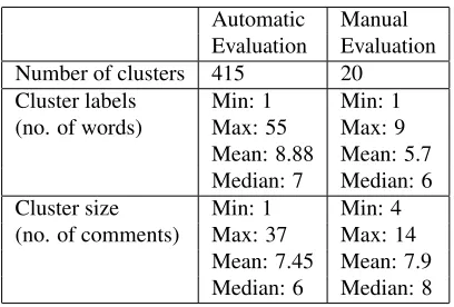
Automatic Manual Evaluation Evaluation

Number of clusters 415 20

Cluster labels Min: 1 Min: 1

(no. of words) Max: 55 Max: 9

Mean: 8.88 Mean: 5.7 Median: 7 Median: 6

Cluster size Min: 1 Min: 4

(no. of comments) Max: 37 Max: 14 Mean: 7.45 Mean: 7.9 Median: 6 Median: 8

Table 1:Dataset statistics

its parent cluster, e.g. in the above example, the sub-cluster “Global warming” becomes an independent cluster labelled “Climate change: Global warming”. In total, the dataset contains 514 clusters, containing an average 7.88 comments (min: 1, max: 69, me-dian: 6), with 8.53 words on average per label (min: 1, max: 55, median: 6).

We further filtered this data, by eliminating clus-ters whose labels do not reflect thetopicof the clus-ter, e.g. labels such as “Jokes”, “Personal attacks to commenters or empty sarcasm”, “Miscellaneous” or “criticisms”. This resulted in a set of 415 clusters that were used for the automatic evaluation.

For the manual evaluation, we further reduced the pool of clusters to those with a maximum of 14 ments (so that annotators could read all the com-ments prior to assessing the labels), and a minimum of 4 comments (so that annotators had enough data to determine the content of the comments). Lastly, only clusters whose labels contained at most 10 words were allowed, as it is not relevant to compare labels with significant length differences. From this pool, 20 comment clusters were randomly selected. Table 1 provides statistics on the two evaluation sets.

3 Method

Our labeling approach is supervised and we refer to it asSCL (Supervised Cluster Labeler). Using the entire set of manually annotatedGuardian articles, we collect training data to build a regression model for extracting labels for automatic clusters.

To do this we first extract terms2 _{from the}

cle as well as comments and represent them with features. Each term is assigned a score between 0 and 1, where 0 indicates a term that is a poor la-bel for a cluster, and 1 a term that makes an excel-lent label. We obtain the score using human sum-maries generated for theGuardianarticles. For these human summaries we have the information about which sentences in the summary links to which hu-man clusters. If the question is to answer whether the termXis a good label for theY cluster, then we collect the sentences from the human summaries that are linked to thatY cluster and compare that termX

with terms extracted from the summary sentences. The comparison is based on Word2Vec (Mikolov et al., 2013) similarity computation and results in a score that varies between 0 and 1. Following this approach we collect training data consisting of terms represented by features and the similarity score to be predicted. Once we have such training data we use linear regression3_{to train a regression model where}

the combination of the features is based on weighted linear combination.

In the test case, i.e., running the cluster labeling approach on a cluster to generate a new label, we again determine terms from the article and the com-ments, extract features, use the regression model to score the terms and select the best scoring term as the label for that cluster. The next section gives a detailed description of the features we used for rep-resenting candidate labels.

3.1 Features

In the cluster labeling approach we use several fea-tures extracted from the news article and the com-ments. To investigate to what extent our intuition about the relevance of the news article for labelling comment clusters is justified and craft features, we analysed a set of 1.7KGuardiannews articles along with their user generated comments. On average we have 206 comments per news article. From each news article we extracted terms and analysed whether they are also used in the comments. Our analysis shows that 35% of the terms extracted from the news article also occur in the comments. We also found out that on average 55% of terms from

3_{We use Weka’s implementation of linear regression.}

http://www.cs.waikato.ac.nz/ml/weka/

the title, and 60% of terms from the first sentence, were mentioned in the comments. Terms extracted from other parts of the news article (sentences 2 to 6 and sentences after the 6th) were mentioned in the comments in only around 45% and 33% of cases re-spectively. Around 43% of comments mentioned at least one term that was found in the article.

Based on this analysis we derived the following features:

• #Term in title: the number of occurrences of a term in the article title.

• #Term in first sentence: the number of occurrences of a term in the first sentence of the article.

• #Term in sentences 2–6 (first paragraph): the number of occurrences of a term in the article sen-tences 2–6.

• #Term in sentences after 6 (main text body): the number of occurrences of a term in the final portion of the article (from the 7th sentence to the end of the article).

• #Term in the entire article: the number of occur-rences of a term in the entire article.

• Article centroid similarity: the cosine similar-ity (Salton and Lesk, 1968) between the term and the article centroid. The similarity is based on Word2Vec word embeddings: each word is repre-sented by a 400-dimensional word embedding. We use the vectors published by Baroni et al. (2014). To compute the similarity of term:document pair, we remove stop-words and punctuation from each, then query for each remaining word’s vector repre-sentation using the Word2Vec, and create a sum of the word vectors. We use the resulting sum vectors to compute their cosine similarity.

In addition to these article-related features, we also compute the following features:

• Term length: the number of words in the term. • #Term in all comments: the frequency of a term in

all comments given to the article.

• #Term in all comments of cluster: the number of occurrences of a term in all comments of a cluster. • Cluster centroid similarity: the cosine similarity

between the term and the cluster centroid. The sim-ilarity is based on Word2Vec.

• #Term in article + comments: the count of occur-rences of a term in the article and its comments. 4 Evaluation

both, we compare the performance of our proposed methodSCLto our baseline method of tf*idf-based labeling, which is described below.

4.1 Baseline: tf*idf-based labeling

In the baseline approach we extract labels from the cluster using thetf*idf metric from information re-trieval. In our casetf (term frequency) is the number of times a candidate label occurs in a cluster. Theidf

is computed based on the number of ‘documents’ in which the label occurs, where the document set comprises the article’s comment plus an additional 4 documents created by splitting the article into the following parts: title, first sentence, (rest of) first paragraph and the remaining text body (as motivated by the observations in Section 3). The candidate la-bels for a cluster are scored by tf*idf, and the top scoring one selected as the cluster label. For compa-rability with the proposed approach (Section 3) we use terms to represent labels.

4.2 Automatic evaluation

For the automatic evaluation we compare the gold standard labels to the machine generated ones. For this purpose we use cosine similarity with and with-out Word2Vec word embeddings. We chose this ap-proach for two reasons. First, when humans and ma-chine select labels that are the same or very simi-lar, this can be captured by cosine similarity with-out Word2Vec word embeddings. Second, humans and machine labels could have similar meaning but use different words, due to synonymy, in which case the use of Word2Vec word embeddings will help co-sine to capture the semantic similarity between the labels. Because of these reasons we use cosine with and without Word2Vec word embeddings. The co-sine similarity between two labelsL1andL2is

com-puted as follows:

cosine(L1, L2) = _|VV_(L(L1)·V(L2)

1)| ∗ |V(L2)| (1)

where V(.) is – depending on whether Word2Vec embeddings are used – either the word vector hold-ing the frequency counts of the words in the respec-tive label or the 400 dimension Word2Vec vector holding the word embeddings. Stop-words are moved before computing this metric. The metric re-turns a value from 0 (no similarity) to 1 (100%

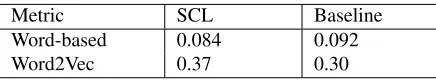
sim-Metric SCL Baseline

Word-based 0.084 0.092

Word2Vec 0.37 0.30

Table 2:Automatic evaluation results

ilar). Overall performance is computed as the aver-age, across all 415 clusters of the evaluation set, of the similarity scores between the automatically se-lected gold standard labels of the cluster

4.3 Manual evaluation

In our manual evaluation, we used an online inter-face where the assessors could first read the news article and assess the quality of the labels based on the scenario shown in Figure 1. Four assessors took part in the evaluation; all were fluent in English and had a background in Computer Science. All asses-sors evaluated the entire set of 20 clusters.

The manual evaluation was divided into three parts. In the first part, assessors were asked to read the comments in the given cluster and to suggest a relevant label to this cluster (referred to as “assessor labels”). In the second part, three different labels (gold standard label, baseline label, and the label generated using our SCL method) were then shown in a random order. For each label, assessors were asked to answer three questions using a 5-point Lik-ert Scale (1: strongly disagree, 5: strongly agree): i) Q1: I can understand this label, ii) Q2: This label is a complete phrase, and iii) Q3: This label accurately reflects the content of the comment cluster. Lastly, assessors were asked to provide any comments of all the labels they have assessed.

Imagine you want to gain a quick overview of what is said in the comments of the news article, but have only a limited amount of time (e.g. a coffee break). The system groups comments into clusters (relating to the same topic), and provides a label, which is a word or phrase that briefly indicates the content of the cluster. A good label should give you a sense of the topics discussed in a cluster, perhaps helping you to decide whether or not to read those comments.

5 Results

5.1 Automatic evaluation results

The results of the automatic evaluation are shown in Table 2. From the table we can see that both base-line and the proposed approach achieve very simi-lar scores measured using cosine without Word2Vec embeddings. Both scores are below 10% indicat-ing that they have very little word overlap between the gold standard labels. When Word2Vec embed-dings are used we see the SCL method achieves higher Word2Vec cosine similarity than the baseline method. The difference between the methods is also significant (p < 0.05).4 _{According to this SCL is a}

better choice in terms of automatic cluster labeling.

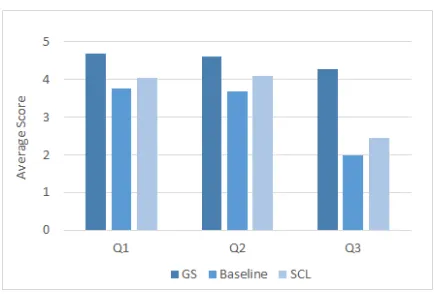
5.2 Manual evaluation results

We gathered judgments of 20 cluster labels from each method: gold-standard (GS), baseline, and SCL. This results in the judgments of 60 cluster la-bels given by each assessor. These lala-bels were eval-uated on three aspects as described in Section 4.3. Figure 2 shows the average scores given by the four assessors for the evaluation questions, where Q1 identifies whether the label can be understood, Q2 represents the phrase completeness of the label, and Q3 represents the accuracy of the label. As we can see from the results the average scores with respect to the Q1 and Q2 are for both the baseline and our SCL method close to the gold label scores. This shows that both automatic labels can be understood and that they are both complete phrases. The re-sults for the Q3, however, are for both systems much lower than the gold label figures. The baseline sys-tem achieves on average 1.98, the SCL 2.43 and the gold labels 4.26. The results between the baseline and SCL present a stable bias across all questions towards the SCL method. In all questions the SCL method outperforms the baseline approach by on av-erage 0.27-0.45 points.

We measure inter-assessor agreement using Krip-pendorff’s alpha coefficient.5_{Agreements in Q1 and}

Q2 are 0.423 and 0.372, respectively, while, higher

4_{Signficance was computed using a one-tailed Studentt-test.} 5_{Scores were computed using R, with the default ’ordinal’} weighting that punishes larger disagreements more than smaller ones. For example, a disagreement between scores 1 and 3 is punished more than that between 1 and 2.

Figure 2: Average scores (4 assessors) on a scale 1:strongly disagree to 5:strongly agree. Questions: Q1:I can understand this label, Q2:This label is a complete phrase, Q3:This label accurately reflects the content of the comment cluster.

agreement ofα= 0.699 is achieved in Q3. Overall, 91.67% cases in Q3 were assigned the identical or a majority score by the four assessors. These figures were 88.3% and 85% for Q1 and Q2, respectively.

Disagreements in Q1 occurred when the labels in-cluded errors or were grammatically incorrect, such as ‘threat so network rail’. The assessors differed in their judgment as to whether the error was relevant to their understanding of the label. A further source of disagreement in Q1 were general labels (‘design stage’), or abstract labels (‘bath of snobbery’).

5.3 Discussion

The automatic comparison between the machine generated labels and the gold standard ones shows that our proposed method significantly outperforms the baseline approach and is a better choice for au-tomatic cluster labeling. This is also confirmed by the manual evaluation figures where again the SCL method outperforms the baseline approach. The cor-respondence between automatic and manual evalua-tion results shows that the Word2Vec based cosine similarity is able to capture the performance differ-ences between different labelling systems.

On the manual evaluation side, Figure 2 shows that both the baseline and the SCL methods perform similar to the gold standard labels with respect to questions Q1 and Q2. However, in case of the Q3 their results substantially differ from the gold stan-dard figures.

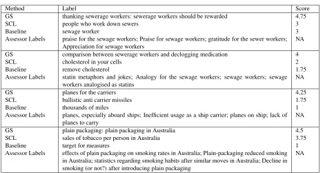
to understand the reasons for this. The error anal-ysis reveals that labels which summarise the over-all discussion in the cluster have been more-highly rated than labels that pick up only a specific men-tion of that discussion. For instance, row 1 of Table 3 shows labels generated for a cluster talking about sewage workers. The gold standard (GS) label cap-tures the essence of the discussion that they should be rewarded for their job, and so provides a good summary of the overall discussion. The automatic methods also capture that the discussion is about the sewage workers, but are not able to abstract it to summarise the entire discussion. From the asses-sor labels provided by our four judges during eval-uation we can see that they label clusters using the same strategy followed by the annotators who gen-erated the gold standard labels.6 _{The labels shown}

in rows 2 and 3 of the table display the same ten-dency. Again the automatic labels capture a specific part of a discussion and fail to summarise it, while manually generated labels (both GS and assessor la-bels) provide a gist of the discussion. This clearly shows that good labels go beyond mere extraction of specific facts, and that automatic labeling systems should seek to more abstractly characterise content. The performance difference between the SCL and the baseline method is most of the time due to the ability of capturing the topic discussed. Although in most cases the baseline method is able to pick up a specific topic relevant key word from a discussion, it fails to do this in few cases. Rows 3 and 4 of Table 3 show examples of such case. We can see that the baseline labels are somewhat related to the discussion however, it is not clear what they refers to. On the other hand the SCL labels do cover a specific part of a discussion completely.

Another reason is that the lengths of the automat-ically generated labels are generally shorter than the gold-standard labels, as shown in Table 4. The aver-age number of words in the baseline labels and SCL labels are 2.7 and 4.55, whilst the human-proposed labels, i.e. the GS and assessor labels were much longer: an average of 5.7 and 6 words, respectively. This finding shows that additional words are needed to summarise the comment clusters more accurately.

6_{Note that the assessors did not see any labels before} pro-viding these labels for comment clusters.

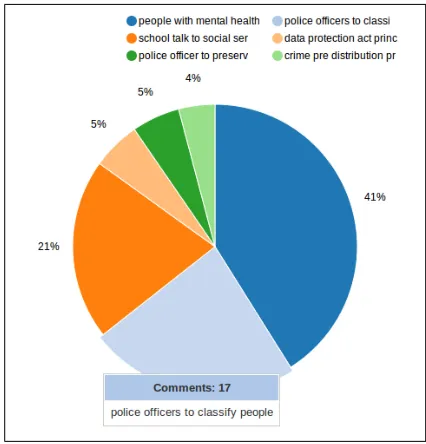
Figure 3:Pie chart

6 Application of cluster labels

Cluster labels can be used for various applications. In this section we describe how cluster labels can be used for summarisation, and we present two alter-native summary formats: a pie chart summary and an abstractive summary. Both summary types could be used by readers of online news to quickly access the content of reader comments instead of browsing through entire comment threads, as in the current set up of commenting forums.

6.1 Pie chart summary

We use a pie chart to present a graphical summary of the clusters. The slices represent the clusters with the labels marking the slices. Figure 3 shows a typi-cal pie chart with 6 clusters.

Method Label Score GS thanking sewerage workers: sewerage workers should be rewarded 4.75

SCL people who work down sewers 3

Baseline sewage worker 3

Assessor Labels praise for the sewage workers; Praise for sewage workers; gratitude for the sewer workers;

Appreciation for sewage workers NA

GS comparison between sewerage workers and declogging medication 4

SCL cholesterol in your cells 2

Baseline remove cholesterol 1.75

Assessor Labels statin metaphors and jokes; Analogy for the sewage workers; sewage workers; sewage

workers analogised as statins NA

GS planes for the carriers 4.25

SCL ballistic anti carrier missiles 1.75

Baseline thousands of miles 1

Assessor Labels planes, especially aboard ships; Inefficient usage as a ship carrier; planes on ship; lack of

planes to carry NA

GS plain packaging: plain packaging in Australia 4.5

SCL sales of tobacco per person in Australia 3.75

Baseline target for measures 1

Assessor Labels effects of plain packaging on smoking rates in Australia; Plain-packaging reduced smoking in Australia; statistics regarding smoking habits after similar moves in Australia; Decline in smoking (or not?) after introducing plain packaging

NA

Table 3:Error analysis: example labels along with their average judgment scores. ‘Assessor Labels’ lists the labels proposed by each of the four assessors, separated by “;”.

Min Max Avg Median

GS 1 9 5.7 6

SCL 3 7 4.55 4

Baseline 2 5 2.7 2

Assessor Labels 1 13 6 6

Table 4:Comparison of label lengths

first showing only the label and the proportion of the comments that fall in each cluster, but it also enables the user to access the full content of the cluster by just clicking the slice.

6.2 Abstractive summary

In addition to the pie chart summary we also gener-ate an abstractive summary. Similar to the pie chart summary the cluster information is used to generate the abstractive summary. The input to the abstractive summariser are the clusters along with their labels. Using this input our summariser applies the follow-ing steps to generate the summary:

1. Ordering the labels: Each cluster comes with a la-bel generated by the SCL method (see Section 3). The clusters are sorted according to their size, i.e. the number of comments.

2. Selecting patterns in which to embed labels: In this setup our aim is to write a sentence for each

la-bel. For this we have written a pool of patterns such as “Most of the comments talk about the topic . . . ”, or “A good amount of contributors discuss the mat-ter . . . ”, etc. Based on the size of the clusmat-ter a pat-tern from the patpat-tern pool is automatically selected and expanded with the label of that cluster. This process proceeds through cluster labels in descend-ing order of cluster size.

3. Selecting example sentences from the cluster: Fi-nally, we select for each cluster label an example sentence extracted from the comments of that clus-ter. To do this we construct the centroid vector rep-resentation of the entire cluster. The vector is based on Word2Vec and sums the vectors of all candidate labels within that label. This sum vector is then compared to Word2Vec vectors of individual sen-tences using cosine. The sentence that has the high-est cosine similarity to the centroid is selected as the example sentence. In the summary the sentences extracted as example follow the generated sentences containing the pattern and the cluster label.

Most of the comments talk about the topic “people with mental health issues”. For example people say “My brother in law has a number of mental health issues including paranoid schizophrenia.”

A good amount of contributors discuss the matter “police officers to classify people”. An example of such discussion is “The police aren’t doctors and they shouldn’t try to be.”

Some people also share their opinions about the topic “police access”. An example of such opinion is “This is sadly what can happen when the police become involved with the vulnerable.” Moreover what difference would it have made had the police access to his records?”

Furthermore, a few discussions entail the subject “school talk to social services”. E.g. “Do you actually know what data social services and the police hold about you and whether it’s accurate?”

Another few mention the topic about “data protection act principles”. A good example for this is the comment extract “Don’t forget we are talking about sensitive personal data here.”

In addition, some minor discussions are about the topic “police officer to preserve freedom”. An examplar of such discussion is “It should be recognised as the duty of every police officer to preserve freedom.”

Figure 4:Example abstractive summary.

access to the associated comment set. In the future we plan to expand the summary with two example sentences to each cluster label to also encode stance (agreement/disagreement) information. We aim to include an agreeing and a disagreeing sentence with respect to the cluster label.

7 Conclusions

In this paper we investigated cluster labeling for clusters containing reader comments to online news. Our labeling approach employs a feature set that in-cludes both features capturing properties local to the cluster and features that capture aspects from the news article and from comments outside the clus-ter. The features are weighted and linearly com-bined. Feature weights are trained using gold stan-dard data and linear regression. To assess the qual-ity of the proposed approach (SCL) we compared it against a tf*idf based baseline using an automatic and a manual evaluation. Both evaluations showed that the SCL outperforms the baseline system. We also demonstrated how cluster labels can be used to provide cluster summaries and presented a pie chart and abstractive summary generated directly from the clusters and their labels.

In future we will focus on the limitations of the current studies: We aim to improve our proposed SCL method and aim to generate labels that take into consideration the entire discussion rather than pick-ing a specific fact from it. With respect to the appli-cation areas we aim to enhance our comment cluster summaries with stance information. Similarly we aim to include sentiment information to capture the

emotions expressed in the comments. On the manual evaluation track we aim to increase our gold stan-dard data. This will help us to draw more reliable conclusions about the different methods.

Acknowledgments

This work was carried out as part of the EU-funded FP7 SENSEI project, grant number FP7-ICT-610916.

References

Ahmet Aker, Monica Lestari Paramita, Emma Barker, and Robert J Gaizauskas. 2014. Bootstrapping term extractors for multiple languages. In LREC, pages 483–489.

Ahmet Aker, Emina Kurtic, Balamurali A R, Mon-ica Paramita, Emma Barker, Mark Hepple, and Rob Gaizauskas. 2016. A graph-based approach to topic clustering for online comments to news. In Proceed-ings of the 38th European Conference on Information Retrieval.

Nikolaos Aletras, Timothy Baldwin, Jey Han Lau, and Mark Stevenson. 2014. Representing topics labels for exploring digital libraries. InProceedings of the 14th ACM/IEEE-CS Joint Conference on Digital Libraries, pages 239–248. IEEE Press.

Emma Barker, Monica Paramita, Ahmet Aker, Emina Kurtic, Mark Hepple, and Robert Gaizauskas. 2016. The SENSEI annotated corpus: Human summaries of reader comment conversations in on-line news. In Proceedings of The 17th Annual SIGdial Meeting on Discourse and Dialogue (SIGDIAL 2016).

compari-son of context-counting vs. context-predicting seman-tic vectors. InACL (1), pages 238–247.

Shuo Chang, Peng Dai, Jilin Chen, and Ed H Chi. 2015. Got many labels?: Deriving topic labels from multi-ple sources for social media posts using crowdsourcing and ensemble learning. InProceedings of the 24th In-ternational Conference on World Wide Web Compan-ion, pages 397–406. International World Wide Web Conferences Steering Committee.

Ioana Hulpus, Conor Hayes, Marcel Karnstedt, and Derek Greene. 2013. Unsupervised graph-based topic labelling using dbpedia. In Proceedings of the sixth ACM international conference on Web search and data mining, pages 465–474. ACM.

Shafiq Joty, Giuseppe Carenini, and Raymond T Ng. 2013. Topic segmentation and labeling in asyn-chronous conversations. Journal of Artificial Intelli-gence Research, pages 521–573.

Elham Khabiri, James Caverlee, and Chiao-Fang Hsu. 2011. Summarizing user-contributed comments. In ICWSM.

Jey Han Lau, Karl Grieser, David Newman, and Timothy Baldwin. 2011. Automatic labelling of topic models. InProceedings of the 49th Annual Meeting of the As-sociation for Computational Linguistics: Human Lan-guage Technologies-Volume 1, pages 1536–1545. As-sociation for Computational Linguistics.

Zongyang Ma, Aixin Sun, Quan Yuan, and Gao Cong. 2012. Topic-driven reader comments summarization. In Proceedings of the 21st ACM international con-ference on Information and knowledge management, pages 265–274. ACM.

Qiaozhu Mei, Xuehua Shen, and ChengXiang Zhai. 2007. Automatic labeling of multinomial topic mod-els. InProceedings of the 13th ACM SIGKDD inter-national conference on Knowledge discovery and data mining, pages 490–499. ACM.

Tomas Mikolov, Ilya Sutskever, Kai Chen, Greg S Cor-rado, and Jeff Dean. 2013. Distributed representa-tions of words and phrases and their compositionality. InAdvances in neural information processing systems, pages 3111–3119.

G. Salton and M. Lesk, E. 1968. Computer evaluation of indexing and text processing. InJournal of the ACM, volume 15, pages 8–36, New York, NY, USA. ACM Press.