Dynamical Systems
Thesis by
Ka-Veng Yuen
In Partial Fulfillment of the Requirements for the Degree of
Doctor of Philosophy
California Institute of Technology Pasadena, California
2002
EARTHQUAKE ENGINEERING RESEARCH LABORATORY
MODEL SELECTION IDENTIFICATION AND ROBUST
CONTROL FOR DYNAMICAL SYSTEMS
BY
KA-VENG YUEN
REPORT No. EERL 2002-03
PASADENA, CALIFORNIA
©
2002Ka- Veng Yuen
Acknowledgements
I would like to express my sincere gratitude and appreciation to my advisor, Prof. James 1. Beck, for his enthusiastic guidance and his support throughout the course of my research. His continuous availability along with many open-minded dis-cussions, are greatly appreciated. I would also like to thank my committee members, Prof. Joel W. Burdick, Prof. John F. Hall, Prof. Wilfred D. Iwan and Prof. Erik A. Johnson, for their valuable comments and suggestions.
;VIy studies are supported by the Cal tech teaching assistantship, the Harold Hell-wig Fellowship and the George 'IV. Housner Fdlowship. These generous supports are gratefully acknowledged.
Special thanks are due to Prof. Lambros S. Katafygiotis, Prof. Costas Papadim-itriou and Prof. Guruswami Ravichandran for their continuous encouragement and support.
;VIy sincere appreciation goes to Ivan Au, Paul Lam, Swami Krishnan, Arash Yavari, ;VIortada ;VIehyar, Fuling Yang, Victor Kam, Lawrence Cheung and Donald Sze for their warm friendships, which have made my graduate life colorful and lively.
Abstract
To fully exploit new technologies for response mitigation and structural health moni-toring, improved system identification and controller design methodologies are desir-able that explicitly treat all the inherent uncertainties. In this thesis, a probabilistic framework is presented for model selection, identification and robust control of smart structural systems under dynamical loads, such as those induced by wind or earth-quakes. First, a probabilistic based approach is introduced for selecting the most plausible class of models for a dynamical system using its response measurements. The proposed approach allows for quantitatively comparing the plausibility of differ-ent classes of models among a specified set of classes.
Then, two probabilistic identification techniques are presented. The first one is for modal identification using nonstationary response measurements and the second one is for updating nonlinear models using incomplete noisy measurements only. These methods allow for updating of the uncertainties associated with the values of the parameters controlling the dynamic behavior of the structure by using noisy response measurements only. The probabilistic framework is very well-suited for solving this nonunique problem and the updated probabilistic description of the system can be used to design a robust controller of the system. It can also be used for structural health monitoring.
Contents
Acknowledgements
Abstract
List of Figures
List of Tables
1 Introduction
1.1 System Identification 1.2 Structural Control . 1.3 Overview of this Thesis .
2 Model Selection
2.1 Overview ..
2.2 "'lodel Class Selection.
2.2.1 Comparison with Akaike's Approach 2.3 Model Updating Using a Bayesian Framework 2.4 Illustrative Examples . . . .
2.4.1 Example 2-1: Single-degree-of-freedom :\fonlinear Oscillator
un-iii iv ix xiii 1 1 5 7 8 8 8 13 13 16
der Seismic Excitation . . . . . 16 2.4.2 Example 2-2: Linear Two-story F\'ame under Seismic Excitation 20 2.4.3 Example 2-3: Ten-story Shear Building under Seismic Excitation 26
2.5 Conclusion. . . .
3 Modal Identification Using Nonstationary Noisy Measurements
3.1 Overview...
3.2 Hmllulation for Modal Identification
28
30
3.3
3.2.2 Parameter Identification Using Bayes' Theorem
:\fumerical Examples . . . .
3.3.1 Example 3-1: Transient Response of SDOF Linear Oscillator
3.3.2 Example 3-2: Eight-story Shear Building Subjected to
:\fonsta-tionary Ground Excitation
3.4 Conclusion...
33
38
38
42
49
4 Updating Properties of Nonlinear DynamicaI Systems with Uncertain Input 50
4.1 Overview.. 50
4.2 Introduction
4.3 Single-degree-of-freedom Systems
4.3.1 Bayesian System Identification FmTllulation
4.3.2 Bayesian Spectral Density Approach
4.4 :Vlultiple-degree-of-freedom Systems
4.4.1 "'lodel Formulation . . . . .
50 53 53 54 57 57
4.4.2 Spectral Density Estimator and its Statistical Properties 58
4.4.3 Identification Based on Spectral Density Estimates 61
4.5 :\fumerical Examples . . . 63
4.5.1 Example 4-1: Dulling Oscillator 63
4.5.2 Example 4-2: Elasto-plastic Oscillator
4.5.3 Example 4-3: Four-story Yielding Structure
4.6 Conclusion. . . .
5 Stochastic Robust Control
5.1 Overview . . . .
5.2 Stochastic Response Analysis
5.3 Optimal Controller Design . .
5.3.1 Conditional Failure Probability
5.3.2 Robust Failure Probability
5.4 Illustrative Examples . . . .
5.4.1 Example 5-1: Four-story Building under Seismic Excitation. 88
5.4.2 Example 5-2: Control Benchmark Problem. 101
5.5 Conclusion . . . .
6 lllustrative Example of Robust Controller Design and Updating
6.1 Problem Description . . . . 6.2 "'lodel Selection and Identification. 6.3 Controller Design . . . .
7 Conclusion and Future Work
7.1 Conclusion.. 7.2 Fllture Work.
A Asymptotic Independence ofthe Spectral Density Estimator
A.1
A.2
A.3
A.4
Bibliography
1J~};Il(W) with 1J~;Il(WI)
urn)
(0 .)
with uUJ)(0
,I)(l,v)l W (l,v)l W •
1J~};Il(w) with 1J~;I(WI) ,( n,iJ)
(0 .)
with ,( 7,6)(0 ./)
"y;!¥ W "y;!¥ w
107
108
108 108 114
123
123 124 126 126 129 130 131
List of Figures
2.1 Relationship between the restoring force and the displacement of the bilinear hysteretic system (Example 2-1). . . . . 16 2.2 Response measurements of the oscillator for the three levels of
excita-tion (Example 2-1). . . . . 17 2.3 Hysteresis loops of the oscillator for the three levels of excitation
(Ex-ample 2-1). . . . 18 2.4 Linear two-story structural frame (Example 2-2). 20 2.5 Response spectrum estimated by the measurements and the best fitting
curve using "'lodel Class 1 (Example 2-2).
2.6 Response spectrum estimated by the measurements and the best fitting curve using Model Class 2 (Example 2-2).
2.7 Response spectrum estimated by the measurements and the best fitting curve using Model Class 3 (Example 2-2).
2.8 Ten-story shear building (Example 2-3).
2.9 Response spectrum estimated by the measurements and the best fitting curve using six modes (Example 2-3) ..
3.1 Measured time history (Exam pIe 3-1).
3.2 Contour of the updated joint PDF of frequency w" and damping ratio 23
23
24 25
28
38
( (Example 3-1). . . . 39 3.3 Marginal updated joint PDFs of the damping ratio ( and the spectral
intensity Sf" (Example 3-1). . . . . 40 3.4 Conditional PDFs of the natural frequency and damping ratio obtained
3.6 Displacement spectral density estimates for the 4th and 9th floor
(Ex-ample 3-2).
3.7 lVlarginal updated joint PDF of natural frequencies WI and W2 (Example
44
3-2). . . . . 46 3.8 Conditional PDFs of the lower two natural frequencies obtained from:
i) Eqn. 3.15 - cross; and ii) Gaussian approximations - solid. The remaining parameters are fixed at their optimal values (Example 3-2). 47
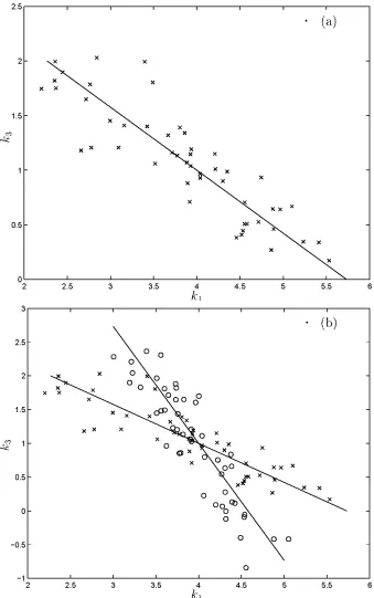
4.1 Schematic plots for identification of Dulling oscillator using the ap-proadl by Roberts et a!. (1995): (a) Data from same level of excita-tion; and (b) Data from two different levels of excitation
(+
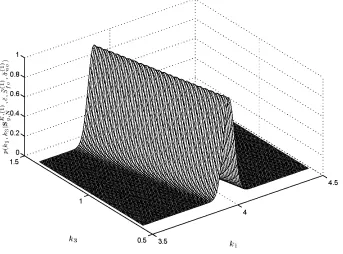
as in (a) and 0 new level). .. . . 52 4.2 Conditional updated PDF p(k"klIS~::~'),t\,S';:!,iTh;)) (Example 4-1). 64 4.3 Conditional updated PDFsP(k"
klIS~::~n),t\
,S';~), iTh~»),n=
1,2(Ex-ample 4-1). . . . 65 4.4 Conditional PDFs of
kl
andkl
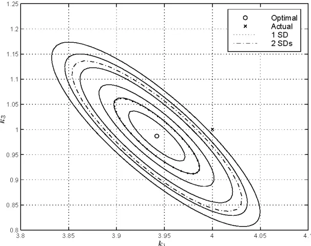
calculated using: i) Eqn. 4.14 - crosses;and ii) Gaussian approximation - solid. The remaining parameters are fixed at their optimal values (Example 4-1). . . . 67 4.5 Contours in the
(k" kl )
plane of conditional updated PDFp( kl'
klIS~::~'),AI(,(2),'(I)'(2),(I),(2) .. " ,_
Sy,N
,t,
S fo , S fo ,Cf~o ,Cf~o) (Example 4 1). . . .4.6 Relationship between the restoring force and the displacement of the system (Example 4-2). . . . . .
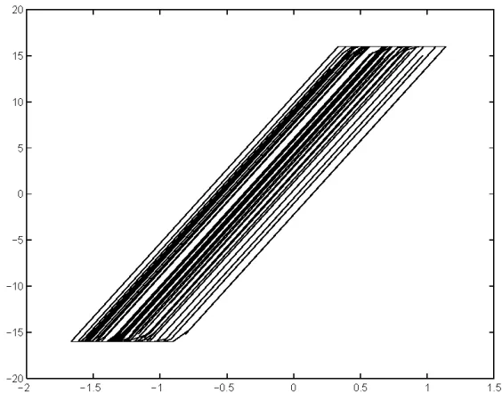
4.7 Hysteresis loops of the simulated data (Example 4-2).
4.8 Contours of marginal updated PDF
P(k"
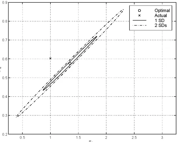
Xy IS~;N) with the theoreticalspectrum estimated by equivalent linearization (Example 4-2). 4.9 Spectral estimates using the measurements (Example 4-2) . . . 4.10 Contours of marginal updated PDF p(Xy, Cfx IS~;N) with the theoretical
67
69 69
71 72
spectrum estimated by equivalent linearization (Example 4-2). . . . . 72
4.11 Contours of marginal updated PDF
P(k"
Xy IS~;N) with the theoreticalspectrum estimated using simulation (Exam pIe 4- 2). . 73 4.13 HJUr-story yielding structure (Example 4-3). . . 75 4.14 Displacement measurements at the 2nd and 5th floor (Example 4-3). 76
4.15 Hysteresis loops for the fourth story (Example 4-3). . . 77 4.16 Spectral estimates and their expected values (Example 4-3). 77 4.17 Contours of marginal updated PDF in the (It I ,lt2 ) plane (Example 4-3). 79
5.1 HJUr-story shear building with active mass driver on the roof (Example 5-1). . . . . 89 5.2 Simulated interstory drifts for the uncontrolled (dashed) and controlled
structure using Controller 1 (solid) (Example 5-1). . . . . 94 5.3 Simulated interstory drifts for the uncontrolled (dashed) and controlled
structure using Controller 2 (solid) (Example 5-1). . . . . 95 5.4 Simulated interstory drifts for the uncontrolled (dashed) and controlled
structure using Controller 3 (solid) (Example 5-1). . . . . 96 5.5 Simulated interstory drifts for the uncontrolled (dashed) and controlled
structure using Controller 4 (solid) (Example 5-1). . . . . 97 5.6 Controller stroke time histories using Controllers 1 - 4 (Example 5-1). 98 5.7 Controller force (normalized by the actuator mass) time histories using
Controllers 1 - 4 (Example 5-1). . . . . 99 5.8 Structural response of the uncontrolled (dashed) and controlled
struc-ture using Controller 3 (solid) to the El Centro earthquake record (Ex-ample 5-1).
5.9 Structural response of the uncontrolled (dashed) and controlled struc-ture using Controller 2 (solid) to the El Centro and Hachinohe
earth-100
quake records (Example 5-2). . . . 105 5.10 Actuator displacement using Controller 2 to the El Centro and
Hachi-nohe earthquake records (Example 5-2). 106
6.2 6.3
Candidate mode! classes (Example 6-1).
Updated PDFs of the rigidity parameters for "'lode! Class A obtained from: i) Eqn. 3.15 - cross; and ii) Gaussian approximations - solid
110
(Example 6-1). . . . 112 6.4 Updated PDFs of the rigidity parameters for Mode! Class B obtained
from: i) Eqn. 3.15 - cross; and ii) Gaussian approximations - solid
(Example 6-1). . . . 113
6.5 Structure-actuator mode! (Example 6-1). 115
6.6 Interstory drift time histories of the uncontrolled structure under twice the 1940 El Centro earthquake record (Example 6-1). . . . . 120 6.7 Interstory drift time histories of the controlled structure under twice
the 1940 El Centro earthquake record (Example 6-1: post-test controller). 121 6.8 Controller stroke time histories under twice the 1940 El Centro
earth-quake record (Example 6-1: post-test controller). 122 6.9 Controller force (normalized by the actuator mass) time histories under
List of Tables
2.1 Optimal (most probable) parameter values in each model class repre-senting the oscillator (Example 2-1). . . . 19 2.2 Probabilities of different model classes based on data (Example 2-1). . 19 2.3 Optimal (most probable) structural parameter values in each model
class representing the structural frame (Example 2-2). . . . . 22 2.4 :\fat ural frequencies (in Hz) of the best model in each class (Example
2-2). . . . . 22 2.5 Probabilities of different model classes based on data (Example 2-2). . 24 2.6 Identified natural frequencies in rad/sec of the building (Example 2-3). 27 2.7 Probabilities of models with different number of modes based on data
(Example 2-3). . . . 27
3.1 Identification results for one set of data and Np
=
20 (Example 3-1).. 39 3.2 Identification results using 100 sets of data and Np= 20 (Example 3-1). 41
3.3 Identification results for the eight-story shear building usingnonsta-tionary approach (Example 3-2).. . . . . 45 3.4 Identification results for the eight-story shear building using
nonsta-tionary approach with acceleration measurements (Example 3-2). 46 3.5 Identification results for the eight-story shear building using stationary
approach (Example 3-2). . . . . 48
4.1 Comparison of the actual parameters versus the optimal estimates and their statistics for the Dulling oscillator (Example 4-1). . . . . 66 4.2 Identification results for the elasto-plastic system with the theoretical
spectrum estimated by equivalent linearization (Example 4-2). . . . . 70 4.3 Identification results for the elasto-plastic system with the theoretical
4.4 Identification results for the four-story yielding building (Example 4-3). 78
5.1 Gain coefficients of the optimal controllers (Example 5-1). 91 5.2 Robust failure probability (Example 5-1). . . 91 5.3 Statistical properties of the performance quantities (Example 5-1). 93 5.4 Design parameters of the optimal controllers (Example 5-2). . . . 102 5.5 Performance quantities for the benchmark problem (Example 5-2). . 103
6.1 Optimal (most probable) structural parameters in each model class representing the structural frame (Example 6-1). . . . . 111 6.2 :\fat ural frequencies (in Hz) of the optimal model in each class (Example
6-1). . . . . 111 6.3 Statistical properties of the performance quantities under random
ex-citation (Example 6-1). . . . . 118 6.4 Statistical properties of the performance quantities under twice the
1940 El Centro earthquake (Example 6-1). . . 119 6.5 Gain coefficients of the optimal controllers (Example 6-1). 119 6.6 Statistical properties of the performance quantities under random
Chapter 1 Introduction
The goal of this work is to develop a complete probabilistic procedure for robust controller design for smart structures that treats all the inherent uncertainties, and includes new system identification techniques that allow the robust controller design to be improved if dynamic data from a structure is available.
1.1 System Identification
The problem of system identification of structural or mechanical systems USlllg dynamic data has received much attention over the years because of its importance in response prediction, control and health monitoring (:\fatke and Yao 1988; Housner et a!. 1997; Ghanem and Sture (Eds.) 2(00).
the data and the noise in the data might have an important role in the data fitting. Therefore, in model class selection, it is necessary to penalize a complicated model.
This was recognized early on by Jeffreys (1961) who did pioneering work on the application of Bayesian methods. He pointed out the need for a quantitative expres-sion of the very old philosophy of 'Ockham's razor' which in this context implies that simpler models are more preferable than unllt'cessarily complicated ones, that is, the selected class of models should accurately describe the behavior of the system but be as simple as possible. Box and Jenkins (1970) also emphasize the same principle when they refer to the need for parsimonious models in time-series forecasting, although they do not give a quantitative expression of their principle of parsimony. Akaike (1974) recognized that maximum likelihood estimation is insufficient for model order selection in time-series forecasting using ARlVIA models and came up with another term to be added to the logarithm of the likelihood function that penalizes against parameterization of the models. This was later modified by Akaike (1976) and by Schwarz (1978).
In recent years, there has been a re-appreciation of the work of Jeffreys (1961) on the application of Bayesian methods, especially due to the expository publications of Jaynes (1983). In particular, the Bayesian approach to model selection has been further developed by showing that the evidence for each model class provided by the data, i.e., the probability of getting the data based on the whole model class, automatically enforces a quantitative expression of a principle of model parsimony or of Ockham's razor (Gull 1988; lVlackay 1992; Sivia 1996). There is no need to introduce ad-hoc penalty terms as done in some of the earlier work on model selection. In Chapter 2, the Bayesian approach is expounded and applied to select the most plausible class of dynamic models representing a structure from within some specified set of model classes by using its response measurements. The model class selection procedure is explained in detail. Examples are presented using a single-degree-of-freedom bilinear hysteretic system, a linear two-story frame and a linear ten-story shear building, all of which are subjected to seismic excitation.
measurements. ,VIuch attention has been devoted to the identification of modal pa-rameters of linear systems without measuring the input time history, such as in the case of ambient vibrations. In an ambient vibration survey, the naturally occurring vi-brations of the structure (due to wind, traffic, micro-tremors, etc.) are measured and then a system identification technique is used to identify the small-amplitude modal frequencies and modeshapes of the lower modes of the structure. The assumption usu-ally made is that the input excitation is a broadband stochastic process adequately modeled by stationary white noise. ,VIany time-domain methods have been developed to tackle this problem. One example is the random decrement technique (Asmussen et a!. 1997) which is based on curve-fitting of the estimated random decrement func-tions corresponding to various triggering condifunc-tions. Several methods are based on fitting directly the correlation functions using least-squares type of approaches (Beck et a!. 1994). Different AR,VIA based methods have been proposed, e.g., Gersch and Foutch (1974); Gersch et a!. (1976); Pi and ,VIickleborough (1989); and Andersen and Kirkergaard (1998). ,VIethods based on the extended Kalman filter method have been proposed to estimate dynamic properties such as natural frequencies, modal damping coefficients and participation factors, of a linear multiple-degree-of-freedom (lVIDOF) system (Gersch and HJUtch 1974; Beck 1978; Hoshiya and Saito 1984; Quek et a!. 1999; Shi et a!. 2(00).
A common assumption in modal identification using response measurements only is that the responses are stationary. However, there are many cases where the re-sponse measurements are better modeled as nonstationary, e.g., a series of wind gusts or in the case of measured seismic response. In the literature, there are very few approaches which tackle modal identification using nonstationary response data, e.g., Safak (1989); Sato and Takei (1997). These methods rely on a forgetting factor for-mulation, which has been demonstrated to be difficult to choose. A bad choice of this forgetting factor will lead to poor results.
ex-ample, how precisely are the values of the individual parameters pinned down by the measurements made on the system? Probability distributions may be used to describe this uncertainty quantitatively and so avoid misleading results (Beck and Katafygiotis 1998). Also, if the identification results are used for damage detection, this proba-bility distribution for the identified model parameters may be used to compute the probability of damage (Vanik et a!. 2(00).
A Bayesian probabilistic system identification framework has been presented for the case of measured input (Beck and Katafygiotis 1998). In Chapter 3, a Bayesian time-domain approach is presented for the general case of linear lVIDOF systems using nonstationary response measurements. The proposed approach allows for the direct calculation of the probability density function (PDF) of the modal parameters which can be then approximated by an appropriately selected multi-variate Gaussian distribution. The importance of considering the response to be nonstationary is also discussed.
System identification using linear models is appropriate for the small-amplitude ambient vibrations of a structure that are continuously occurring. There is, however, a number of cases in recent years where the strong-motion response of a structure has been recorded but not the corresponding seismic excitation. In some cases this is be-cause of inadequate instrumentation of the structure and in other cases it is bebe-cause the free-field or base sensors malfunctioned during the earthquake. Fm' example, the seismic response was recorded in several steel-frame buildings in Los Angeles which were damaged by the 1994 :\forthridge earthquake, but analysis of these im-portant records has been hampered by the fact that the input (base motions) were not recorded and also because of the strong nonlinear response.
exten-sion of the case of measured input (Beck and Katafygiotis 1998; Katafygiotis et a!. 1998). The proposed spectral-based approach utilizes important statistical proper-ties of the Fast Fourier Transform (FFT) and their robustness with respect to the probability distribution of the response signal, e.g., regardless of the stochastic model for this signal, its FFT is approximately Gaussian distributed. The method allows for the direct calculation of the probability density function (PDF) for the param-eters of a nonlinear model conditional on the measured response. The formulation is first presented for single-degree-of-freedom (SDOF) systems and then for multiple-degree-of-freedom systems. Examples using simulated data for a Dulling oscillator, an elasto-plastic system and a four-story yielding structure are presented to illustrate the proposed approach.
1.2 Structural Control
Because complete information about a dynamical system and its environment are never available, system and excitation parameters can not be determined exactly but can be given probabilistic descriptions which give a measure of how plausible the possible parameter values are (Cox 1961; Beck 1996; Beck and Katafygiotis 1998). Classical control methods based on a single nominal model of the system may fail to create a controller which can provide satisfactory performance for the system. Robust control methods, e.g., ?i2 , ?iN and It-synthesis, etc., were therefore proposed so that
Over the last decade, there has been increasing interest in probabilistic, or stochas-tic, robust control theory. ,VIonte Carlo simulations methods were used to synthesize and analyze control systems for uncertain systems (Stengel and Ray 1991; "-'Larrison and Stengel 1995). In Spencer and Kaspari (1994); Spencer et a1. (1994); Field et a1. (1994); and Field et a1. (1996), first- and second-order reliability methods were incorporated to compute the probable performance of linear-quadratic-regulator con-trollers (LQR). On the other hand, an efficient asymptotic expansion (Papadimitriou et a1. 1997a) was used to approximate the probability integrals that are needed to determine the optimal parameters for a passive tuned mass damper (Papadimitriou et a1. 1997b) and the optimal gains for an active mass driver (May and Beck 1998) for robust structural control. In May and Beck (1998), the proposed controller feeds back output measurements at the current time only, where the output corresponds to certain response quantities that need not be the full state vector of the system. However, there is additional information from past output measurements which may improve the performance of the control system.
In Chapter 5, the reliability-based methodology proposed in May and Beck (1998) is extended to allow feed back of the output (partial state) measurements at previous time steps. It is noted that in traditional linear-quadratic-Gaussian (LQG) control with partial state measurements, the optimal controller can be achieved by estimating the full state using a Kalman filter combined with the optimal LQG controller for full state feedback. However, in our case the separation principle does not apply and no state estimation is needed. The method presented for reliability-based robust control design may be applied to any system represented by linear state-space models but the focus here is on robust control of structures (Soong 1990; Housner et a1. 1997; Caughey (Ed.) 1998).
model and a benchmark structure are given to illustrate the proposed approach.
1.3 Overview of this Thesis
1. Chapter 2 introduces a probabilistic approach for selecting the most plausible class of models for a structure using dynamic data.
2. Chapters 3 and 4 introduce two identification techniques for linear systems using nonstationary response measurements and for nonlinear systems with uncertain input.
3. Chapter 5 introduces a stochastic robust control methodology, with considera-tion of modeling uncertainty, structure-actuator interacconsidera-tion and time delay of the controller.
4. Chapter 6 illustrates the proposed robust controller design framework using a 2()-DOF four-story structural frame.
Chapter 2 Model Selection
2.1 Overview
A Bayesian probabilistic approach is presented for selecting the most plausible class of models for a structure within some specified set of model classes, based on structural response data. The crux of the approach is to rank the classes of structural models based on their probabilities conditional on the response data which can be calculated based on Bayes' Theorem and an asymptotic expansion for the evidence for each model class. The approach provides a quantitative expression of a principle of model parsimony or of Ockham's razor which in this context can be stated as simpler models are to be preferred over unllt'cessarily complicated ones. Examples are presented to illustrate the method using a single-degree-of-freedom bilinear hysteretic system, a linear two-story frame and a ten-story shear building, all of which are subjected to seismic excitation.
2.2 Model Class Selection
Let 1) denote the input-output or output-only dynamical data from a structure. The goal is to use 1) to select the most plausible class of models representing the structure out of NM given classes of models jlv/ I, jlv/2, ... ,jlv/"'M' Since probability
where p(VIU)
=
LJ:~ p(VIA1j,U)P(A1jIU) by the theorem of total probability and U expresses the user's judgement on the initial plausibility of the model classes, expressed as a prior probability P(A1j IU) on the model classes A1j, j=
1, ... , NM ,where LJ:~ P(A1jIU)
=
1. The factor p(VIA1j,U) is called the evidence for the model class A1j provided by the data V. :\fote that U is irrelevant in p(VIA1j, U) and so it can be dropped in the notation because it is assumed that A1j alone specifies the probability density function (PDF) for the data, that is, it specifies not only a class of deterministic structural models but also the probability descriptions for the prediction error and initial plausibility for each model in the class A1j (Beck and Katafygiotis 1998). Eqn. 2.1 shows that the most plausible model class is the one that maximizes p(VIA1j)P(A1jIU) with respect to j.:\fote that P(A1jIV,U) can be used not only for selection of the most probable class of models, but also for response prediction based on all the model classes. Let
u denote a quantity to be predicted, e.g., first story drift. Then, the PDF of u
given the data V can be calculated from the theorem of total probability as follows:
p(uIV, U)
=
LJ:~ p(uIV, A1j)P(A1j IV, U), rather than just using only the best model for prediction. However, if P(A1bestlV, U) for the best model class is much larger than others, then the above expression is approximated by p(uIV, U)=
p(uIV, A1best) and it is sufficient to just use the best model class.The evidence for A1j provided by the data V is given by the theorem of total probability:
where OJ is the parameter vector in a parameter space E>j C lRNj that defines each
model in A1j, the prior PDF p( OJ IA1j) is specified by the user and the likelihood p(VIA1j, OJ) is calculated using the methods introduced in Section 2.3, Chapter 3 and Chapter 4.
Gaussian distribution, so p('DIAij) can be approximated by using Laplace's method for asymptotic approximation (Papadimitriou et a!. 1997a):
where Nj is the number of uncertain parameters for the model class Aij, the
op-timal parameter vector OJ is the most probable value (it is assumed to maximize
p((Jjl'D, Aij) in the interior of E>j) and Hj(Oj) is the Hessian matrix of the function
-In[p('Dl9j, Aij)p((JjIAij)] with respect to (Jj evaluated at OJ. For nnident'(fiable
cases (Beck and Katafygiotis 1998), the evidence p('DIAij) can be calculated by us-ing an extension of the asymptotic expansion used in Eqn. 2.3 (Beck and Katafygiotis 1998; Katafygiotis et a!. 1998) or by using a :VIarkov chain :VIonte Carlo simulation technique (Beck and Au 2(02) on Eqn. 2.2. The discussion here will focus on the
globally ident'(fiable case.
The likelihood factor p('DIOj, Aij) in Eqn. 2.3 will be higher for those model classes Aij that make the probability of the data 'D higher, that is, that give a better 'fit' to the data. For example, if the likelihood function is Gaussian, then the highest value of p('DIOj, Aij) will be given by the model class Aij that gives the smallest least-squares fit to the data. As mentioned earlier, this likelihood factor favors model classes with more uncertain parameters. If the number of data points N in 'D is large, the likelihood factor will be the dominant one in Eqn. 2.3 because it increases exponentially with N, while the other factors behave as N-I
, as shown below.
. . -~ _!'!...i -~ j . _
The remaIllIllg factors p((JjIAij)(21f) 2 IHj((Jj)I-' III Eqn. 2.3 are called the Ock-hom factor by Gull (1988). The Ockham factor represents a penalty against param-eterization (Gull 1988; :VIackay 1992), as we demonstrate in the following discussion.
matrix Hj (9j ). The principal posterior variances for (Jj, denoted by O},i with i
=
1,2, ... ,Nj , are therefore the inverse of the eigenvalues of this Hessian matrix. The• l
determinant factor IHj((Jj)I-' in the Ockham factor can therefore be expressed as the product of all the OJ,i for i
= 1,2, ...
,Nj . Assume that the prior PDF p((JjIAij) is Gaussian with mean (most probable value a priori) OJ and a diagonal covariance matrix with variances P],i with i= 1,2, ...
,Nj • The logarithm of the Ockham factor for the model class Aij, denoted by3
j , can therefore be expressed as(2.4)
Since the prior variances will always be greater than the posterior variances if the data provides any information about the model parameters in the model class Aij,
all the terms in the first sum in Eqn. 2.4 will be positive and so will the terms in the second sum unless the posterior most probable value OJ,i just happens to coincide with the prior most probable value OJ,i' Thus, the log Ockham factor 3j will decrease
if the number of parameters Nj for the model class Aij is increased. Furthermore,
since the posterior variances are known to be inversely proportional to the number of data points N in
1),
the dependence of the log Ockham factor on N is3j
= -
~
In N Nj+
Rj (2.5)where the remainder Rj depends primarily on the choice of prior PDF and is 0(1) for large N. It is not difficult to show that this result holds for even more general forms of the prior PDF than the Gaussian PDF used here.
It follows from Bayes' Theorem that we have the exact relationship:
(2.6)
data provides any information about the model parameters in the model class Aij. Indeed, for large N, the negative of the logarithm of this ratio is an asymptotic approx-imation of the information about OJ provided by data V (Kullback 1968). Therefore, the log Ockham factor 3j removes the amount of information about OJ provided by
V from the log likelihood Inp(VIOj, Aij) to give the log evidence p(VIAij).
The Ockham factor may also be interpreted as a measure of robustness of the model class Aij. If the updated PDF for the model parameters for the given model class is very peaked, then the ratio p(OjIAij)!p(OjIV,Aij), and so the Ockham fac-tor, is very small. But a narrow peak implies that response predictions using this model class will depend too sensitively on the optimal parameters
OJ.
Small errors in the parameter estimation will lead to large errors in the results. Therefore, a class of models with a small Ockham factor will not be robust to noise in the data during parameter estimation, that is, during selection of the optimal model within the class. :\fote that Inp(VIOj, Aij) and the log Ockham factor 3j are approximately proportional to N and In N, respectively, where N is the number of data points in V.Therefore, as N becomes larger, the contribution of the log Ockham factor becomes less important. This is reasonable because the uncertainty in the values of the model parameters becomes smaller as the number of data points grows, that is, the param-eters can be estimated more precisely if more data points are available. In this case, the model class can be less robust since we are more confident about the values of the parameters of the model class.
To summarize, in the Bayesian approach to model selection, the model classes are ranked according to p(VIAij)P(AijIU) for
.i
=
1, ... ,NM , where the best class ofmodels representing the system is the one which gives the largest value of this quantity. The evidence p(VIAij) may be calculated for each class of models using Eqn. 2.3.
The prior distribution P(Aij IU) over all the model classes Aij,
.i
= 1, ...
,NM , must2.2.1 Comparison with Akaike's Approach
In the case of Akaike's information criterion (Akaike 1974), the best model class among the Aij for
.i
=
1,2, ... ,NM is chosen by maximizing an objective functionAIC(Aij IV) over
.i
that is defined by(2.7)
where the log-likelihood function is roughly proportional to the number of data points
N in V, while the penalty term is taken to be Nj , the number of adjustable parameters
in the model class Aij. (Akaike actually stated his criterion as minimizing -2(AIC) but the equivalent form is more appropriate here). 'When the number of data points is large, the first term will dominate. Akaike (1976) and Schwarz (1978) later developed independently another version of the objective function, denoted BIe, that is defined by
(2.8)
where now the penalty term increases with the number of data points N.
BIe can be compared directly with the logarithm of the evidence from Eqn. 2.3:
(2.9)
where the logarithm of the Ockham factor
3
j is given by Eqn. 2.4 or Eqn. 2.5. The latter shows that for large N, the BIe agrees with the leading order terms in the logarithm of the evidence and so in this case it is equivalent to the Bayesian approach using equal priors for all of the P(AijIUj ).2.3 Model Updating Using a Bayesian Framework
A general Bayesian framework for structural model updating was proposed III
pre-sented using input-output measurements. In this section, this Bayesian approach for linear/nonlinear model updating is presented. Fm' details, see Beck and Katafygiotis (1998). The case of using output only measurements is covered later in Chapter 3 (linear models) and Chapter 4 (nonlinear models).
Consider a system with Nd degrees of freedom (DOFs) and equation of motion
(2.10)
where M E lR"" X " " is the mass matrix, f" E lR"" is the nonlinear restoring force
characterized by the structural parameters (J,,, T E lR"" X"! is a force distributing matrix and f(t) E lR"! is an external excitation, e.g., force or ground acceleration, which is assumed to be measured.
Assume now that discrete response data are available for No(~ N d) measured DOFs. Let::"t denote the sampling time step. Because of measurement noise and modeling error, referred to hereafter as prediction error, the measured response y(n) E lR"o (at time t
=
n::"t) will differ from the model response Lox(n) corresponding to the measured degrees of freedom where Lo denotes an No x Nd observation matrix, comprised of zeros and ones. Herein, it is assumed that this difference between the measured and model response can be adequately represented by a discrete zero-mean Gaussian white noise vector process 'T/ (n) E lR"o:y(n)
=
Lox(n) +'T/(n) (2.11 )where the discrete process 'T/ satisfies
(2.12)
where
E[.]
denotes expectation, <lnp denotes the Kronecker delta function, and I;'1 denotes the No x No covariance matrix of the prediction error process 'T/.mass distribution; 3) the elements of the force distributing matrix T; and 4) the elements of the upper right triangular part of the prediction-error covariance matrix I;~ (symmetry defines the lower triangular part of this matrix). Herein, it is assumed that the mass distribution can be modeled sufficiently accurately from structural drawings and so it is not part of the model parameters to be identified.
If the data 1) consists of the measured time histories at N discrete times of the excitation and observed response, then it is easily shown that the most probable values
iJ
of the model parameters are calculated by minimizing the mean square error between the measured and computed model response at the observed DOFs because of the assumed probability model for the prediction error. Assuming that the prediction errors have equal variance (J~ but are independent for different channels of measurements, the updated PDF of the model parameters (J given dynamic data1) and model class jlv/ is given by
(2.13)
where Cl is a normalizing constant and p( (Jljlv/) is the prior PDF of the model param-eters (J expressing the user's judgement about the relative plausibility of the values of the model parameters before data is used. The objective function J1 ((JI1), jlv/) is
given by
(2.14)
where x(k::"t; (J, jlv/) is the calculated response based on the assumed class of models and the parameter set (J and y(k::"t) is the measured response at time k::"t, respec-tively. Furthermore, 11.11 denotes the 2-norm of a vector. The most probable model parameters
iJ
are obtained by maximizing p((JI1),jlv/) in Eqn. 2.13. For large N, this is equivalent to minimizing J1 ((JI1), jlv/) in Eqn. 2.14 over all parameters in (J that it-Iy
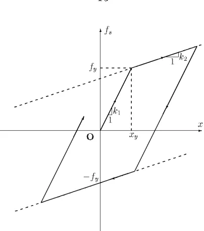
Figure 2.1: Relationship between the restoring force and the displacement of the bilinear hysteretic system (Example 2-1).
case (Beck and Katafygiotis 1998), it turns out that p(9IV,A-t) is well approximated by a Gaussian distribution with mean
9
and covariance matrix equal to inverse of the Hessian of -In[p(9IV,M)]
at9.
2.4 Illustrative Examples
2.4.1 Example 2-1: Single-degree-of-freedom Nonlinear Oscillator
under Seismic Excitation
In this example, a bilinear hysteretic oscillator with linear viscous damping is considered:
(2.15)
where Tn is the mass, c is the damping coefficient and
!h
(x; kl' k2' Xy) is the hystereticrestoring force, whose behavior is shown in Fig. 2.1. Here, Tn
= 1kg is assumed known.
[image:31.612.222.424.56.284.2]~
-~ ;:"
o 05r--~-~r--~-~---,-,r-____ ~--~---,
10% El Ceniro e,:u1 hquake
-0 050L--~-~,LO -~'5'----~20'----~25---=30---=35--40
~
-~ ;:"
o 05r--~-~r--~-~----;:7CCc-:c~--co-r---'
15% El Ceniro e;tr1 hquake
-0 050~----O---7,""0 ---;,5,----~20,---;C25---=30,---=35---:40
o 05r--~-~r--~-~----;:T:-____ ~--~ ____ --'
20% El Ceniro e;::u1 hquake
15 20 25
t (sec) 30 35 40
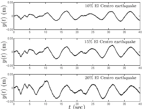
Figure 2.2: Response measurements of the oscillator for the three levels of excitation (Example 2-1).
1.0 :-J/m, k2
=
O.n/m, Xy 0.02 m, which gives a small-amplitude natural frepuencv of -2' Hz.'1 '-' 1T
The oscillator is assumed to be excited by 10%, 15% and 20% of the 1940 El Centro earthquake record. The duration of measurement is T
= 40 sec with sampling
frequency 60Hz, so that the number of data points is N=
2400. It is assumed that the earthquake excitation and response displacement are measured to give the data 1) where 5% rms noise is imposed on the structural response measurements, i.e., the measurement noise is 5% of the rms of the noise-free response. Fig. 2.2 shows the measurements for the three levels of excitation and Fig. 2.3 shows the corresponding hysteresis loops. It can be seen that the oscillator behaved linearly (did not yield) when subjected to 10% of the El Centro earthquake record. Three classes of models are considered. They all use zero-mean Gaussian discrete white noise as the prediction-error model."'lodel Class 1 (Ai,): Linear oscillators with damping coefficient c
>
0, stiffness parameter k,>
0 and predictive-error standard deviation (J~; [image:32.612.186.457.81.290.2]005
~ 10% El Ceniro e;;u1 hquake
?
---~ ~ -~ ~ -005-0 O~ -003 -002 -001 001 002 003 00'
005
~ 15% El Ceniro €i\r1 hquake
?
=
~ ~ 0
-~ ~
-005
-0 O~ -003 -002 -001 001 002 003 00'
005
~ 20% El Ceniro e;;u1 hquake
? ~ ~
-
-~ ~ -005-0 O~ -003 -002 -001 o 001
x(t) (m) 002 003 00'
Figure 2.3: Hysteresis loops of the oscillator for the three levels of excitation (Example 2-1 ).
k2
= 0, with stiffness parameter
kl>
0, yielding level Xy and predictive-error standarddeviation (J~; and no viscous damping.
"'lodel Class 3 (Ai:)): bilinear hysteretic oscillators with pre-yield stiffness kl
>
0, after yielding stiffness k2>
0, yielding level Xy and predictive error parameter (Jw:-Jote that this class of models does not include the exact model since linear viscous damping is not included.
Independent uniform prior distributions are assumed for the parameters c, k1, k2 ,
Xy and (J~ over the range (O,O.5):-J sec/m, (O,2):-J/m, (O,O.5):-J/m, (O,O.I)m, (O,O.01)m,
respectively. Table 2.1 shows the optimal parameters of each class of models for the three levels of excitation. 'U:-J' indicates that the parameter is unidentifiable. Fm' example, in jVj2 with 10o/r; El Centro earthquake, Xy is unidentifiable because the
oscillator behaves perfectly linearly (Fig. 2.3). In fact, the optimal parameters of
Excitation Level "'lodel Class c kl k2 Xy (J~
1 0.0204 1. 000 0.0005
10% El Centro earthquake 2 1.019 U)J 0.0013
3 1.019 U)J U)J 0.0013
1 0.0902 0.989 0.0020
15% El Centro earthquake 2
un
79 0.0214 0.00173 1.001 (J.108 0.0197 0.0007
1 0.1928 0.956 0.0098
20% El Centro earthquake 2 0.9936 0.0211 0.0051
3 0.9942 0.0924 0.0200 0.0011
Table 2.1: Optimal (most probable) parameter values in each model class representing the oscillator (Example 2-1).
Excitation level P(A'qD,U) P(M211J ,U) P(M l l1J,U)
10% El Centro earthquake 1.0 3.1 x 10 1217 3.1 x 10 1217 15% El Centro earthquake 4.4 x 10 1174 3.2 x 10 957 1.0 20% El Centro earthquake 6.4 x 10 2l0l 5.7x10 IG09
1.0
Table 2.2: Probabilities of different model classes based on data (Example 2-1).
due to yielding.
'" :rr,(1) '" :r,,(1) :r2(1) (I':n:
(1':112 (1':112
:r,,(1) ,:[:(1) :r, (I) (1': I)"
(1': I), (1': I),
(I )
Figure 2.4: Linear two-story structural frame (Example 2-2).
viscous damping, as can be seen by the large increase in the optimal damping ratio for the corresponding "equivalent" linear systems
Ai,
in Table 2.1. Furthermore, the restoring force behavior for ;\12 is more correct than for ;\1" although it is still not exact.This example illustrates an important point in system identification. In reality, there is no exact class of models for a real structure and the best class depends on the circumstances. If we wish to select between the linear models (;\1,) and the elasto-plastic models (;\12), then ;\12 is better for high levels of excitation while ;\1,
is better for lower levels of excitation.
2.4.2 Example 2-2: Linear Two-story Frame under Seismic
Excita-tion
The second example refers to a 6-DOF two-story structural frame with story height H
= 2.5m and width
W=
4.0m, as shown in Fig. 2.4. All the chosen model classes are linear. All members are assumed to be rigid in their axial direction. Fm' each member, the mass is uniformly distributed along its length. The rigidity-to-mass ratio is chosen to be i:'i:=
i:'i2=
i:'ia=
i:'i4=
2252m4 sec-2 where Tn denotes themass per unit length of all members. As a result, the first two natural frequencies of this structure are 2.000Hz and 5.144Hz. Furthermore, a Rayleigh damping model is assumed, i.e., the damping matrix C
=
exM+ 3K, where
M and K are the mass and stiffness matrices, respectively. In this case, the nominal values of the damping coefficients cl; and j are chosen to be 0.182 sec- I and 0.442 x 1O-:l sec so that the damping ratios for the first two modes are l.OOo/r;.Three classes of structural models are considered. Independent zero-mean discrete Gaussian white noise is used for the prediction-error model, with spectral intensity Snl
= O.027m2 sec:l and Sn2
= O.059m2 sec:l at the two observed degrees offreedom.
In order to have better scaling, the damping parameters are parameterized as follows:ex
=
(;)Ji and 3=
(;)23."'lodel Class 1 (A11): Assumes a class of two-story shear buildings with nominal interstory stiffness kl
=
k2=
2 xI~f:'.
In order to have better scaling, the stiffness are parameterized as follows: kj=
(ljkj,.i=
1,2. Therefore, the uncertain parameters are (lj, (;)j, Snj, .i= 1,2.
Model Class 2 (A12): Assumes the actual class of models except that due to modeling error, Ell
=
(lIEl l , Eh=
(l2El2, El:l=
O.5(1IEl:l and El4=
O.5(12El4, where the nominal values were given earlier. Therefore, the uncertain parameters are (lj, (;)j and Snj, .i= 1,2.
Model Class 3 (A1:l): Assumes that Ell
=
(lIEl l , Eh=
(l2El2 and Elj=
(I:lElj,.i=
3,4. Therefore, the uncertain parameters are: (II, (12, (I;), (;)1, (;)2, Snl and Sn2. :\fote that the true model lies in this set.The structure is assumed to be excited by a white noise ground motion, which is not measured. The spectral intensity of the ground motion is taken to be So
=
1.0 x 1O-5m2 sec3 The data 1) consists of the absolute accelerations with 10o/r; measurement noise at the 1"t and 2nd DOFs over a time interval of 100 sec, using a sampling interval of (J.(ll sec. Identification was performed using the Bayesian spectral density approach of Chapter 4 with the same set of data for each of the three classes of models.uniform distribution over the interval (0,2) for (I" (12, (I:), (;)" (;)2 and over the interval
(0, O.5)m2 sec3 for Sn' and Sn2.
Parameter Ct'l (;'2 (I, (12 (13
8
n1 8n2Case 1 1.131 1.007 0.913 0.879 0.158 0.159 Case 2 1.057 1.536 1.130 1.130 0.150 0.063 Case 3 1.027 1.093 0.988 1.0(Jl 1.024 0.085 0.080
Table 2.3: Optimal (most probable) structural parameter values in each model class representing the structural frame (Example 2-2).
"'lode 1 2 Actual 2.000 5.144 Case 1 2.048 5.009 Case 2 2.000 5.323 Case 3 1.995 5.142
Table 2.4: :\fatural frequencies (in Hz) of the best model in each class (Example 2-2).
Table 2.3 shows the optimal structural parameters in each class of models. It is not surprising that both (I, and (12 in Case 1 are less than unity because the shear building models assume a rigid floor but the floors of the actual structure are not. Table 2.4 shows the associated natural frequencies with the actual frame and the op-timal models. :\fote that the opop-timal model in
Ai3
can fit both frequencies very well since the exact model is in this class. On the other hand,Ai,
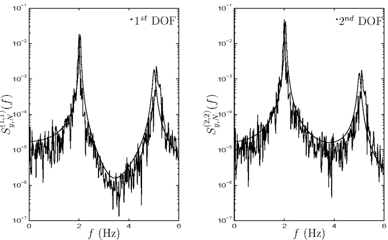
and jVi2 can not fit thefrequency of the second mode as well as jVi3 . Fig. 2.5 - 2.7 show the estimated spec-trum using the measurements (zigzag curve) with the best fitting specspec-trum (smoother curve) for the three classes of models, respectively. One can see that the best model in jVi2 provides a better fit to the first mode than jVi" but it is the opposite for the
second mode. The best model in jVi3 gives excellent matching with the estimated spectrum for both modes.
10-1 r----~---~---_____, 10-1 r----~---~----_,
10-7 L -_ _ _ ~ _ _ _ ~ _ _ _ _____' 10-7L-_ _ _ ~ _ _ _ ~ _ _ _ _ _'
0 2 4 6 0 2 4 6
f
(Hz)f
(Hz)Figure 2.5: Response spectrum estimated by the measurements and the best fitting curve using "'lode! Class 1 (Example 2-2).
10-1 r----~---~---_____, 10-1 .---~---~---,
10-7 L - - - o : - - - c - - - ' 0 2 4 6
f
(Hz)10-7':---o:----~:_---_: 0 2 4 6
f
(Hz) [image:38.612.125.521.84.329.2]10-1 r---~---~---____' 10-1 r----~--~---____,
10-7 L -_ _ ~ _ _ _ ~ _ _ _ ____' 10-7 L -_ _ _ ~ _ _ ~ _ _ _ ____'
0 2 4 6
f
(Hz)0 2 4 6
f
(Hz)Figure 2.7: Response spectrum estimated by the measurements and the best fitting curve using "'lodel Class 3 (Example 2-2).
As expected, P(A13IV,U) is the largest among the three classes of models because it contains the actual model. On the other hand, P(A1
IIV,
U) is the smallest one. Although it gives a better fit for the second mode than ;\12, it does not fit the first mode as well as the best model in ;\12 and the contribution of the first mode to the structural response is one order of magnitude larger than the second mode. This implies that although ;\12 has significant modeling error for the beams (about 50%), it is still a better class of models than the shear building models.P(MIIV,U) P(M2IV ,U) P(M 3IV ,U)
2.6 x 10 23 1.7xl0 15 1.0
!I( t)
~ .. - - - . . g(t)
2.4.3 Example 2-3: Ten-story Shear Building under Seismic
Excita-tion
The third example uses response measurements from the ten-story building shown in Fig. 2.8. The Bayesian approach is applied to select the optimal number of modes for a linear model. It is assumed that this building has a uniformly distributed floor mass and storv stiffness over its height. The stiffness to mass ratios ,/ n~j kj,'j .!
= 1, ... ,4,
are chosen to be 1500 sec2
so that the fundamental frequency of the building is 0.9213 Hz. Rayleigh damping is assumed, i.e., the damping matrix C is given by C
=
exM +[)K, where ex=
0.0866 seC I and [)= 0.0009 sec. The structure is assumed
to be subjected to a wide-band random ground motion, which can be adequately modeled as a Gaussian white noise with spectral intensity Sio
= 0.02m2
sec3 :\fote that the matrix T in Eqn. 2.10 is equal to the matrix -[ml, ... ,mlOf in this case. Each model class Ai)Ci
=
1, ... ,8) consists of a linear modal model (Beck 1996) with j modes and the uncertain parameters are the natural frequency, damping ratio and modal participation factor for each mode; and the spectral intensity Sn of the prediction error at the measured degree of freedom.The data 1) consists of the absolute accelerations at the top floor with 5% mea-surement noise over a time interval T
=
30 sec, using a sampling interval ::"t=
(J.(ll sec. The measurement noise is simulated using a spectral intensity Sn=
1.94 x 1O-4m2 sec 3 The Bayesian spectral density approach of Chapter 4 is used for the identification. The number of data points N is taken to be 600 because only the estimated spectrum up to 20.0 Hz is used.Independent prior distributions for the parameters are taken as follows: Gaussian distribution for the natural frequencies with mean 5.5(2j -1) rad/sec and coefficient of variation 0.05 for the jth mode. Furthermore, the damping ratios, modal participation factor and the spectral intensity of the modeling error are assumed to be uniformly distributed over the range (0,0.05), (0,2) and (0, 0.(1)m2 sec:l, respectively.
:-lumber of modes WI 0)2 W:J 0)4 W5 WG 0)7 W8
Exact 5.789 17.24 28.30 38.73 48.30 56.78 64.00 69.79
1 6.946
2 5.799 20.68
3 5.814 17.16 33.96
4 5.842 17.18 27.94 43.82
5 5.848 17.19 27.97 38.06 50.58
6 5.849 17.19 27.97 38.09 48.10 56.72
7 5.849 17.19 27.97 38.09 48.13 56.34 64.18
8 5.849 17.19 27.97 38.09 48.13 56.34 64.18 69.41
Table 2.6: Identified natural frequencies in rad/sec of the building (Example 2-3).
:-lumber of modes Tn 1 2 3 4
Inp(VIA1m) 1.894 x 1():l 2.251 X 1():l 2.511 X 1():l 2.619 X 1():l
In
.Bra
-43.7 -56.4 -68.9 -69.2 P(MmIV,U) 3.0 x 10 TW 2.2 x 10 18G 6.4 x 10 79 2.4 x 10 :l2:-lumber of modes Tn 5 6 7 8
Inp(VIA1m) 2.682 x 1():l 2.714 X 1():l 2.723 X 1():l 2.723 X 1():l
In
.Bra
-75.9 -91.2 -109 -121P(MmIV,U) 1.0 x 10 7 1.0 1.7x10 4 1.3 x 10 9
Table 2.7: Probabilities of models with different number of modes based on data (Example 2-3).
the log-Ockham factor In 3m and P(A1jIV,U)
Ci
=
1, ... ,8) for the cases of modelclasses with one mode to eight modes, calculated from Eqn. 2.1 using the evidence for each model from Eqn. 2.3 and equal priors P(A1jIU)
=
t.
It implies that using six modes is optimal. It is found that the seven-mode and eight-mode models give poor estimation of the damping ratios although the estimated natural frequencies are satisfactory, as shown in Table 2.6. The estimated (most probable) damping ratios of the seventh mode are 15.3% and 17.2%, using the seven-mode and eight-mode models, respectively. The eight-mode model gives 25.9% for the most probable damping ratio for the eighth mode. :-lote that the actual values of the damping ratios of the seventh and eighth mode are 2.86% and 3.10%, respectively.1O'r---.---.---.---r---.---~
Using 6 modes
1 0-5 L -_ _ _ _ -:'::-_ _ _ _ ~___'__ _ _ _ _ ~ _ _ _ _ __'LL'_--'-'-__'_'_LLl___'__-'---JLJ..J
o 20 40 60 80 100 120
W (rad/sec)
Figure 2.9: Response spectrum estimated by the measurements and the best fitting curve using six modes (Example 2-3).
fitting curve using six modes (smoother curve). One can see that the optimal model using six modes can fit the measured spectrum very well. Furthermore, all the six identified natural frequencies are very close to their target values, which is not the case for using two to five modes. It was found that if ArC is used, eight modes is optimal because the penalty term is too small compared to the changing of the log likelihood term in Eqn. 2.7. On the other hand, if BrC in Eqn. 2.8 is used, then six modes are optimal, agreeing with the Bayesian approach using the evidence for the various modal models.
2.5 Conclusion
evidence for the model class provided by the data and the user's choice of prior probability distribution over the classes of models. The methodology can handle input-output and output-only data for linear and nonlinear dynamical systems. This is further illustrated in Chapters 3, 4 and 6.
Chapter 3 Modal Identification Using
N onstationary Noisy Measurements
3.1 Overview
This chapter addresses the problem of identification of the modal parameters for a structural system using measured nonstationary response time histories only. A Bayesian time-domain approach is presented which is based on an approximation of the probability distribution of the response to a nonstationary stochastic excitation.
It allows one to obtain not only the most probable values of the updated modal pa-rameters and stochastic excitation papa-rameters but also their associated uncertainties using only one set of response data. It is found that the updated probability dis-tribution can be well approximated by a Gaussian disdis-tribution centered at the most probable values of the parameters. Examples are presented to illustrate the proposed method.
3.2 Formulation for Modal Identification
3.2.1 Random Vibration Analysis
Consider a system with Nd degrees of freedom (DOF) and equation of motion:
Mi + C
x
+Kx=
ToF(t) (3.1)where M, C and K are the mass, damping and stiffness matrices, respectively; To E
nonstationary stochastic process which is modeled by
F(t)
=
A(t)g(t) (3.2)where g( t) is a Gaussian stationary stochastic process with zero mean and spectral density matrix Sg(w) E lR"F' X"F' and A(t) E lR is a modulation function. Then, the autocorrelation function of F is given by
R/.(t, t
+
7)=
A(t)A(t+
7)Rg(7) (3.3)where Rg(7) is the autocorrelation function for the stationary process g(t).
Assuming classical damping, i.e., CM-'K
=
KM-'C (Caughey and O'Kelly 1965), the uncoupled modal equations of motion by using modal analysis are given byr
= 1, ...
,Nd (3.4)where q(t)
=
[ql (t), ... , q",,(t)f and f(t)=
[II (t), ... ,tv"
(t)f are the modal coordi-nate vector and the modal forcing vector, respectively. The transformation between the original coordinates (forces) and the modal coordinates (forces) is given byx(t)
=
iP, q(t) and f(t)=
(MiP)-'Tog(t) (3.5)where iP is the modeshape matrix, comprised of the modeshape vectors ljJ(T) which
are assumed to be normalized so that
A,(T)
=
1o/1r ' r
=
1, ... ,Nd (3.6)where iT is a measured DOF which is not a node of the rth mode. The modal forcing
matrix
(3.7)
and autocorrelation matrix function
(3.8)
It is known that the response x(t) is a Gaussian process with zero mean, correlation function between Xj and Xl (Lutes and Sarkani 1997):
(3.9)
and with spectral density
(3.10)
where hT (.) denotes the modal unit impulse response function for the displacement of the rth mode. Here, it is assumed that only Nm lower modes contribute significantly
to the displacement response.
Assume that discrete data at times tk
=
k!'lt, k=
1, ... ,N, are available at No(~Nd ) measured DOFs. Also, assume that due to measurement noise and modeling error
there is prediction error, i.e., a difference between the measured response y(k) E lRNo and the model response at time tk
=
k!'lt corresponding to the measured degrees of freedom. The latter is given by Lox(k!'lt) where Lo is an No x Nd observation matrix, comprised of zeros and ones, that is,y(k)
=
Lox(k!'lt) +n(k) (3.11 )zero-mean Gaussian white noise n(k) E IR with the following No x No covariance matrix
T .
-E[n(m)n (p)]
=
I;n')m,p ( 3.12)where <lm,p is the Kroneker Delta function.
:\fote that y(k) is a discrete zero-mean Gaussian process with autocorrelation matrix function Ry given by
Ry(m,p)
=
E[y(m)yT(p)](3.13)
where Rx denotes the autocorrelation matrix function of the model response x(t)
given by Eqn. 3.9, and I;n is the noise covariance.
3.2.2 Parameter Identification Using Bayes' Theorem
Since it is assumed that only Nm lower modes contribute significantly to the
response, only the modal parameters corresponding to these modes are identified. Specifically, the parameter vector a for identification is comprised of: 1) the modal parameters Wn (n r
= 1, ... , N
m in Eqn. 3.4; 2) the modeshape components C;);r) at theobserved DOF
.i
=
1, ... ,No for the modes r=
1, ... ,Nm , except those elementswhich were used for the normalization of the modeshapes (which are assumed constant and equal to one); thus, a total of Nm(No - 1) unknown modeshape parameters are to be identified; 3) the parameters prescribing the spectral density matrix Sg(w) and the modulation function A(t) and 4) the elements of the upper right triangular part of I;n (symmetry defines the lower triangular part of this matrix).
components of the rth modeshape to be scaled by some constant tT; at the same time the values of the elements
sy's)
of the modal forcing spectral density matrix will be scaled by (tTCs )-1.Let the vector Ym,p denote the zero-mean random vector comprised of the response measurements from time m;:"t to p;:"t (m S; p) in a time-descending order, that is,
m S; p (3.14 )
Using Bayes' theorem, the expression for the updated PDF of the parameters a given some measured response Y I,N is
(3.15 )
where C2 is a normalizing constant such that the integral of the right-hand side of
Eqn. 3.15 over the domain of a is equal to unity. The factor pta) in Eqn. 3.15 denotes the prior PDF of the parameters and is based on previous knowledge or engineering judgement; in the case where no prior information is available, this is treated as a constant. plY I,N !a) is the dominant factor in the right-hand side of
Eqn. 3.15 reflecting the contribution of the measured data in establishing the posterior distribution. This can be expanded into a product of conditional probabilities as follows:
N
P(YI,N!a)
=
P(YI,Np!a)II
p(y(k)!a;Y"k-l) ( 3.16)k=:Vf>+1
In order to improve computational efficiency, the following approximation is in-troduced:
N
P(YI,N!a) ~ P(YI,Np!a)
II
p(y(k)!a;Yk-Np,k-l) (3.17)k=:Vp+l
points. The sense of this approximation is that data points belonging too far in the past do not have