THE DYNAMICS OF RINGED
SMALL BODIES
A Thesis Submitted by
Jeremy R. Wood
For the Award of
Doctor of Philosophy
Abstract
In 2013, the startling discovery of a pair of rings around the Centaur 10199 Chariklo opened up a new subfield of astronomy - the study of ringed small bodies. Since that discovery, a ring has been discovered around the dwarf planet 136108 Haumea, and a re-examination of star occultation data for the Centaur 2060 Chiron showed it could have a ring structure of its own.
The reason why the discovery of rings around Chariklo or Chiron is rather shocking is because Centaurs frequently suffer close encounters with the giant planets in the Centaur region, and these close encounters can not only fatally destroy any rings around a Centaur but can also destroy the small body itself.
In this research, we determine the likelihood that any rings around Chariklo or Chiron could have formed before the body entered the Centaur region and survived up to the present day by avoiding ring-destroying close encounters with the giant planets. And in accordance with that, develop and then improve a scale to measure the severity of a close encounter between a ringed small body and a planet.
We determine the severity of a close encounter by finding the minimum dis-tance obtained between the small body and the planet during the encounter, dmin, and comparing it to the critical distances of the Roche limit, tidal
dis-ruption distance, the Hill radius and “ring limit”. The values of these critical distances comprise our close encounter severity scale.
The ring limit is defined as the close encounter distance between a planet and a ringed small body in a hyperbolic or parabolic orbit about the planet for which the effect on the ring is just noticeable in the three-body planar problem. The effect is considered just noticeable if the close encounter changes the orbital eccentricity of the orbit of any ring particle by 0.01. In the first version of our scale, the ring limit is set equal to a constant value of 10 tidal disruption distances for each planet, and the effect of the velocity at infinity,v∞, of the
orbit of the small body about the planet is ignored.
The method of backwards numerical integration of clones is used to deter-mine the time intervals from now backwards in time within which Chariklo and Chiron have been injected into the Centaur region. The results show that Chariklo likely entered the Centaur region during the last 20 Myr and Chiron within the last 8.5 Myr from somewhere in the Trans-Neptunian region. We recorddmin for all close encounters between each clone and each giant planet
during these time intervals and use the severity scale to determine the like-lihood that the close encounters could have destroyed any rings around each body during its time interval.
From this, it is seen that ring-destroying close encounters are so extremely rare that it is statistically likely that each body’s rings could have originated outside the Centaur region assuming that the effects of viscous dispersion are negated by other stabilizing factors such as shepherd satellites and self-gravitating rings.
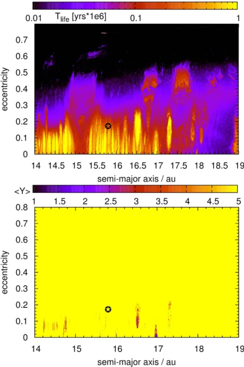
does not. Their half-lifes are 3 Myr and 0.7 Myr respectively.
The accuracy of our close encounter severity scale is improved by finding the ring limits for simulated close encounters between hypothetical one-ringed small bodies and planets in the 3-body planar problem. The effects of planet mass, small body mass,v∞, and ring orbital radius are fully accounted for.
When velocity effects are taken into account, we discover that the ring limit forms a curve indmin−v∞space, the ring limit has a lower bound of
approxi-mately 1.8 tidal disruption distances regardless of the small body mass or ring orbital radius, and that the ring limit equals this lower bound for parabolic orbits only.
Our data is then used to find an analytical solution for a ring limit upper bound curve for Chariklo-planet encounters. We present three different methods for using this curve. To test our results, The ring limits found from all three methods are compared to 27 previously published dmin values for
Chariklo-planet encounters in the seven-body non-planar problem.
Only onedmin value is found to be greater than the ring limit and that all
ring limits are within 4.4 tidal disruption distances for each planet. We conclude that these values are more accurate than the crude value of 10 tidal disruption distances used in the first version of our close encounter severity scale.
Future work is discussed and may include simulations of Chariklo, Chiron or Haumea in which the ring particles and possibly satellites are included.
Certification of Thesis
This Thesis is the work of Jeremy R. Wood except where otherwise acknowl-edged, with the majority of the authorship of the papers presented as a Thesis by Publication undertaken by the Student. The work is original and has not previously been submitted for any other award, except where acknowledged.
Principal Supervisor: Associate Professor Stephen C. Marsden
Associate Supervisor: Professor Jonathan Horner
Associate Supervisor: Dr. Tobias C. Hinse
List of Contributions from Publication Co-authors
• Article I:Wood, J., Horner, J., Hinse, T. C., and Marsden, S. C., (2017). “The Dynamical History of Chariklo and its Rings” Astronomical Jour-nal, vol. 153, pp. 245- 252. (Top 15% journal; Impact Factor: 4.617 and SNIP: 1.32).
DOI: https://doi.org/10.3847/1538-3881/aa6981
The overall contribution of Jeremy Wood was 85% to the concept devel-opment, analysis, drafting and revising the final submission; Stephen C. Marsden, Jonathan Horner and Tobias C. Hinse contributed the other 15% to concept development, analysis, editing and providing important technical inputs.
• Article II:Wood, J., Horner, J., Hinse, T. C., and Marsden, S. C., (2018). “The Dynamical History of 2060 Chiron and its Proposed Ring System” Astronomical Journal, vol. 155, pp. 2 - 14. (Top 15% journal; Impact Factor: 4.617 and SNIP: 1.32).
DOI: https://doi.org/10.3847/1538-3881/aa9930
The overall contribution of Jeremy Wood was 85% to the concept devel-opment, analysis, drafting and revising the final submission; Stephen C. Marsden, Jonathan Horner and Tobias C. Hinse contributed the other 15% to concept development, analysis, editing and providing important technical inputs.
• Article III: Wood, J., Horner, J., Hinse, T. C., and Marsden, S. C., (2018). “Measuring the Severity of Close Encounters Between Ringed Small Bodies and Planets” has been submitted for publication in the Monthly Notices of the Royal Astronomical Society and is currently under review. (Top 19% journal; Impact Factor: 4.961 and SNIP: 1.08). DOI: TBA
Acknowledgments
I would like to express my sincere gratitude to the many people and organiza-tions that aided me in the completion of this degree.
First, I would like to thank George Coyne for his talk on galaxies and Neil Degrasse Tyson for his talk on science illiteracy which gave me the idea of re-turning to school to pursue a degree in astronomy. Tremendous gratitude goes to my co-authors and advising team of Associate Professor Stephen C. Marsden, Professor Jonathan Horner and Dr. Tobias C. Hinse (the dream team!) for their meticulous work on this project and without whose help this degree would not have been possible. I acknowledge their assistance in giving advice, proof read-ing, taking data and project conception. Thanks to the University of Southern Queensland for providing funds to attend conferences and pay publishing fees.
The data for two of the papers in this project were taken using the super-computing facilities at the University of Southern Queensland and stored in Cloudstor. I would like to thank the Australian Access Federation for providing Cloudstor for our use and Francis Gacenga for his technical support with it.
Table of Contents
Abstract ii
Certification of Thesis iv
List of Contributions from Publication Co-authors v
Acknowledgments vi
Table of Contents vii
List of Figures ix
List of Tables x
1 Introduction 1
1.1 A Brief Review of Cosmological Models . . . 1
1.1.1 The Geocentric Model . . . 1
1.1.2 The Copernican Model . . . 2
1.1.3 The Keplerian Model . . . 3
1.1.4 Kepler’s First Law . . . 3
1.1.5 Kepler’s Second Law . . . 3
1.1.6 Kepler’s Third Law . . . 4
1.1.7 The Universality of Kepler’s Laws . . . 4
1.1.8 Newton’s Universal Law of Gravitation . . . 5
1.1.9 Tidal Forces . . . 5
1.2 The N-Body Problem . . . 7
1.2.1 Overview of the N-Body Problem . . . 7
1.2.2 The Solar System N-body Problem . . . 7
1.2.3 The 2-Body Problem in the Solar System . . . 8
1.2.4 The Circular Restricted 3-Body Problem . . . 12
1.3 Resonances . . . 16
1.3.1 Mean Motion Resonances . . . 17
1.3.2 Secular Resonances . . . 20
1.3.3 Resonances and Chaos . . . 21
1.4 Numerical Integrators . . . 23
1.4.1 Euler’s Method . . . 24
1.4.2 Other Integrators . . . 24
1.4.3 The Bulirsh-St¨oer Method . . . 25
1.4.4 The Hybrid Integrator of Mercury . . . 25
1.4.5 The IAS15 Integrator . . . 26
1.4.6 Application of Numerical Integrators . . . 28
1.5 Small Bodies of the Solar System . . . 29
1.5.2 Comets . . . 32
1.5.3 Comet Origins . . . 32
1.5.4 Comet Taxonomy . . . 33
1.5.5 Centaurs . . . 36
1.6 The Effects of Planets on Small Bodies . . . 39
1.7 Ringed Small Bodies . . . 40
1.7.1 Ring Detection . . . 41
1.7.2 Chariklo . . . 43
1.7.3 Chiron . . . 43
1.7.4 Haumea . . . 44
1.8 Research Questions . . . 45
1.8.1 What is the likelihood that the rings of Chariklo could have formed before Chariklo entered the Centaur region? 45 1.8.2 What is the likelihood that any rings of Chiron could have formed before Chiron entered the Centaur region? . . . . 45
1.8.3 How does the ring limit depend on the variables associated with a close encounter between a ringed small body and a planet? . . . 46
2 The Dynamical History of Chariklo and its Rings 47 3 The Dynamical History of 2060 Chiron and its Proposed Ring System 57 4 Measuring the Severity of Close Encounters Between Ringed Small Bodies and Planets 72 5 Conclusions 105 5.1 Chariklo and Chiron . . . 105
5.2 Ring Origins . . . 106
5.3 Measuring Close Encounter Severity . . . 107
5.4 The Future . . . 109
List of Figures
(Excluding figures included in Chapters 3-5)
1.1 The conic sections . . . 9
1.2 An elliptical orbit with true and eccentric anomalies . . . 11
1.3 An elliptical orbit with longitude of ascending node and argument of perihelion . . . 13
1.4 The five Lagrange points . . . 16
1.5 Two nearly identical orbits . . . 22
1.6 Changeover Function . . . 27
1.7 A histogram of small bodies in the inner Solar system . . . 31
1.8 An example of a comet taxonomical scheme . . . 34
1.9 Centaurs in the HEBA scheme . . . 38
1.10 Chariklo Light Curve . . . 41
List of Tables
(Excluding tables included in Chapters 3-5)
1.1 Kepler’s 3rd Law . . . 4
1.2 Conic sections . . . 10
1.3 Eigenfrequencies of the Jovian planets . . . 21
1.4 Trojans . . . 30
1.5 NEAs . . . 31
1.6 The letters for HEBA classes . . . 35
1.7 The HEBA subclasses . . . 36
1
Introduction
From antiquity, human beings have been looking upward at the heavens. The first humans saw the Sun and the Moon - two great lights - and stars that formed shapes in the sky. Every day and night these heavenly objects were seen to constantly move across the sky in an east to west motion relative to the horizon.
As this motion occurred, most stars maintained their position relative to other stars, but some stars were seen to wander – alternating between eastward and westward motion relative to other stars. These wanderers were not stars at all but planets.
But stars and planets were not the only objects our ancient ancestors ob-served. Occasionally these ancient people noticed strange fuzzy objects which appeared in the sky in places where no object had been seen before. They no-ticed that these surprise guests had tails and were larger than any star. Over time, these objects would fade from view. These were the first human sightings of comets – one type of small body in the Solar system.
In a sense, the science of small bodies of the Solar system began with the very first comet sighting. It would be millennia, however, before the exact nature of comets would be understood, and along the way other types of small bodies would be found.
1.1
A Brief Review of Cosmological Models
Humans had been observing the heavens for centuries before any attempt was made at explaining the motions observed. For example, we know that ancient Babylonians observed planets because of records found on clay tablets. As far as we know, the Babylonians had no model in which the planets orbited a central body.
A cosmological model explains heavenly motions and accurately predict fu-ture events. For example, a model could be used to predict the locations of planets on future dates. If the model is good then the planets will appear at the predicted locations on the future dates. If a model is bad then it can either be refined or discarded.
1.1.1 The Geocentric Model
It was the ancient Greeks who first tried to explain the motions they were seeing in the heavens. From the Greeks point of view, everything seemed to revolve around the Earth. Having no computers nor space probes nor even knowledge of gravity we can hardly blame the Greeks for inventing the erroneous geocentric or Earth-centered model.
and was unable to explain why planets changed their angular speed in the sky and occasionally drifted westward relative to the stars in loops and zig zags before resuming their more usual eastward motion.
Over the centuries different incarnations of the geocentric model were for-mulated in an attempt to align all heavenly motion with the model. In an attempt to explain why planets seemed to speed up and slow down in their mo-tion against the stars, Earth was moved off-center of the invisible spheres which contained planets. This centered the motion on a point rather than on Earth, and the changing distance between Earth and the planet explained the change in speed. When the planet was closer to Earth it appeared to move faster in the sky and when farther away appeared to move more slowly. Though if you stood at the center of the planet’s invisible sphere it would seem to maintain the same speed. Having Earth off-center was known as an eccentric. The stars had their own sphere centered on Earth since their motion relative to the horizon was uniform.
Greeks even devised a method to explain retrograde motion of planets while still maintaining spheres spinning in the same direction. They did this by placing the planet on a smaller spinning sphere the center of which was fixed to the rim of a constantly spinning much larger sphere. The larger sphere was called the deferent and the smaller sphere the epicycle.
The most successful geocentric model devised was the Ptolemaic model. In this model, the epicycles of Mercury and Venus were fixed to an Earth-Sun line, and the radii of the epicycles of the other planets were forced to remain parallel to it. The center of the motion was a point exactly off-center opposite of Earth and was called the equant.
1.1.2 The Copernican Model
The Ptolemaic model reigned as the accepted model of the universe until the 16th century when Polish astronomer Nicolaus Copernicus revived a little known ancient Greek model known as the heliocentric model. At that time, the he-liocentric model was contrary to the teachings of the Church. Believing that Earth orbited the Sun could result in your imprisonment, torture, or even death. No wonder that Copernicus’ model was only published just before his death in 1543.
In this model, Earth is replaced as the center of revolution with the Sun. Planets still resided on invisible spheres and still had epicycles though they were smaller than in the Ptolemaic model. Heavenly motions were still explained but in a different way.
1.1.3 The Keplerian Model
Through painstaking analysis of planetary positional data taken by Tycho Brahe, Johannes Kepler determined that the orbits of planets were not circles but were in fact ellipses. With the introduction of ellipses, epicycles were no longer nec-essary. Kepler’s model was also heliocentric as the Copernican model had been, but Kepler abandoned the long-held notion that planets resided on invisible spheres. Instead he introduced for the first time in a cosmological model the idea that a force from the Sun was responsible for holding planets in their orbits. He believed this force was magnetic in nature.
Kepler’s model could predict planetary positions as much as ten times better than the Ptolemaic model making it the best model up to that time. The properties of planetary orbits in Kepler’s model are summarized in what today are called Kepler’s three laws of motion released in 1609, 1609 and 1618.
1.1.4 Kepler’s First Law
Kepler’s first law states that the orbit of each planet is an ellipse with the Sun at one focus. Nothing is at the other focus (Bate et al., 1971; Zeilik, 2002; Bennett et al., 2016; Fraknoi et al., 2016).
An ellipse is the set of points in a plane such that the sum of the distances from each point to two fixed points is a constant. Each fixed point is called a focus. The major axis is a line which runs through both foci and connects the sides of the ellipse. The semi-major axis,a, is half the major axis.
The amount by which an ellipse differs from a circle is called the eccentricity, e, of the ellipse. A circle is a special case of an ellipse for which both foci are located at the same point. A circle has an eccentricity of zero. Givenc is the distance from either focus to the geometrical center of the ellipse, the eccentricity is given by:
e= c
a (1.1)
0≤e <1 for any ellipse.
1.1.5 Kepler’s Second Law
Kepler’s second law states that a line drawn from a planet to the Sun sweeps out equal areas in equal times.
Table 1.1: The modern semi-major axes of the orbits of the eight planets taken from NASA’s Horizon ephemeris for January 1, 2000. Also shown are the orbital periods calculated using Kepler’s 3rd Law and the observed values. Differences between these two are explained by rounding errors.
Planet amodern (au) Pcalculated (years) Pobserved (years)
Mercury 0.387098 0.240842 0.240851
Venus 0.723327 0.61518 0.615204
Earth 1.000372 1.000558 1.000597
Mars 1.523678 1.880788 1.880864
Jupiter 5.205109 11.875303 11.870117
Saturn 9.581452 29.65835 29.655306
Uranus 19.229945 84.327082 84.328634
Neptune 30.096971 165.114107 165.08904
1.1.6 Kepler’s Third Law
Kepler’s third law states that the square of the orbital period of the orbit of a planet, P, is directly proportional to the cube of the orbit’s semi-major axis. The orbital period is the time it takes a planet to orbit the Sun one time (Bate et al., 1971; Zeilik, 2002; Bennett et al., 2016; Fraknoi et al., 2016). This law can be stated as
P2=ka3 (1.2)
Law 3 shows that the larger a planet’s semi-major axis the longer it takes to orbit the Sun and the slower its average orbital speed. If P is in years and a is in astronomical units then k = 1 for all planets orbiting the Sun. Table 1.1 shows the modern semi-major axes of the orbits of the eight planets. Also shown are the orbital periods calculated using Kepler’s 3rd Law and the observed values. The modern semi-major axes were taken from NASA’s Horizon ephemeris service for Jan. 1, 20001.
1.1.7 The Universality of Kepler’s Laws
Though Kepler originally developed his laws for planets orbiting the Sun, today we know that his laws can be applied to any elliptical orbit in the two-body prob-lem for which the orbiting body has negligible mass compared to the primary body. Examples include moons orbiting planets, artificial satellites orbiting a planet, and small bodies orbiting the Sun (Bennett et al., 2016).
1.1.8 Newton’s Universal Law of Gravitation
A better understanding of the physics behind Kepler’s laws arrived with the publication of Isaac Newton’s Principia. In this work, Newton explains three laws of motion and a Universal Law of Gravitation. Today these four laws are part of what is known as Newtonian Mechanics.
In his book, Newton explains his Universal Law of Gravitation using these words: Every point mass in the universe attracts every other point mass in the universe with a force directly proportional to the product of the masses and inversely proportional to the square of the distance between the masses. This can be expressed as:
F =Gcm1m2
r2 (1.3)
(Zeilik, 2002; Bennett et al., 2016; Fraknoi et al., 2016) whereFis the magnitude of the force on each of the two masses,Gc is the gravitational constant of the
universe which is 6.673×10⁻¹¹ Nm2
kg2 in SI units,m1andm2are the point masses, andris the distance between the two point masses.
The Universal Law obeys Newton’s third Law so that each mass feels the same force due to the other but in the opposite direction.
Newton’s Universal Law can be used to find the constantkin equation 1.2. Consider the special case of a small body of massm orbiting the much more massive Sun of massMSun in a circular orbit of radiusr.
In this case the centripetal force is supplied entirely by the gravitational force between the two masses. This equality is written as
mv 2
r =Gc mMsun
r2 (1.4)
Since the speed is constant, the velocity vector,v=2πr
P . This can be combined
with Equation (1.4) to yield:
P2= 4π
2
Gc m+MSun !r
3 (1.5)
For elliptical orbits the result is the same withrreplaced witha.
1.1.9 Tidal Forces
A tidal force is the difference in gravitational force of one body on another across the body in question. The evaluation of a tidal force vector, F~tf, at a
point on a body equals the subtraction of two vectors: the gravitational force experienced by a point mass at the point in question,F~, and the gravitational force experienced by a point mass at the center of mass of the object,F~cm. This
is shown by
As one example of a tidal force calculation, consider a point massmat radial distance r from the center of mass of the small body located at a point on a line between the center of mass of the small body and that of a planet of mass Mp. Assume the small body is not rotating and has no tensile strength. If the
distance between the two centers of mass isdthen Equation (1.6) is written as
Ftf =Gc
mpm
d−r
!2 −Gc
mpm
d2 =Gcmpm
"
1
d−r
!2−
1 d2
#
(1.7)
The Maclaurin expansion of 1
d−r
!2 is ≈ d12 +d2r3. Substituting this into
equation (1.7) yields an approximate form for the tidal force
Ftf ≈Gcmpm "
1 d2 +
2r d3 −
1 d2
#
=2Gcmpmr
d3 (1.8)
The tidal force of a planet on a small body can be strong enough to rip the small body apart. This was the fate of comet Shoemaker-Levy 9 in 1994 as it approached Jupiter and was torn into 21 separate pieces which then collided with the planet (e.g. Harris et al., 1994; Gough, 1994; Loders & Fegley, 1998; Jessup et al., 2000).
The distance between a small body held together by its own gravity and a planet within which the small body can be torn apart by tidal forces is called the Roche Limit. For simplicity, consider the case where the small body is a sphere; and the rotation of the small body and tidal force of the small body on the planet are negligible. When the small body is at the Roche limit distance from the planet (d = Rroche), the gravitational force of the small body on a
point mass on the small body’s surface just equals the tidal force due to the planet on this point mass. Using equation (1.8) to approximate the tidal force, this condition can be expressed as
2Gcmpmr R3
roche
= Gcmsm
r2 (1.9)
Solving forRroche yields the Roche Limit equation
Rroche=r 2mp ms
!13
(1.10)
Equation (1.10) can be rewritten using the densities of the small body and planetρsandρp respectively. Assuming spherical bodies, the result is
Rroche=Rpl 2ρp ρs
!13
whereRpl is the physical radius of the planet. For the special caseρs=ρpthe
Roche limit is about 1.26Rpl. If the deformation of the small body is taken into
account then the result for a tidally locked liquid small body orbiting the planet is (Murray & Dermott, 1999)
Rroche= 2.44Rpl ρp ρs
!13
(1.12)
1.2
The N-Body Problem
1.2.1 Overview of the N-Body Problem
The N-Body problem is the study of the dynamics ofNinteracting point masses. Only the 2-Body problem can be solved analytically for the general case (Murray & Dermott, 1999; Gurfil et al., 2016). The solution to the general case of the 3-Body and larger N-3-Body problems can only be approximated numerically using computer algorithms. The set of point masses under study is called a system.
The state of thenthpoint mass,ψn, can be defined as the set of components
of its position, ~rn, velocity,~vn, and acceleration,~acn, vectors and a value for
time, t. The combined states of all point masses which make up the system define the state of the system, Ψ.
ψn= "
~rnx, ~rny, ~rnz, ~vnx, ~vny, ~vnz, ~acnx, ~acny, ~acnz, t #
(1.13)
Ψ =
""
~r1x, ~r1y, ~r1z, ~v1x, ~v1y, ~v1z, ~ac1x, ~ac1y, ~ac1z, t #
, ... (1.14)
"
~rN x, ~rN y, ~rN z, ~vN x, ~vN y, ~vN z, ~acN x, ~acN y, ~acN z, t ##
1.2.2 The Solar System N-body Problem
The dynamical behavior of the Solar system or part of the Solar system over some period of time can be approximated by considering only the gravitational forces among the members of the system. In this approximation, the effects of relativity and non-gravitational forces are ignored.
To find the net force acting on a single point mass at any moment in time, the net force acting on that mass due to the gravitational forces from all the other point masses must be calculated using
~ Fi=
N−1
X
j=1 ~
Fij (1.15)
wherei6=j. F~i is the net force acting on theith mass, and F~ij is the
equation (1.3). OnceF~iis known, the acceleration of theithmass can be found
using Newton’s 2nd Law.
As a specific example, consider a system containing only two point masses miandmjwith position vectors~riand~rjrespectively. The displacement vector
frommi tomj is~rij =~rj−~ri.
Newton’s Universal Law can be rewritten in vector form to yieldF~ij. To do
this, the concept of the unit vector can be employed. A unit vector of~rij has a
magnitude of 1 and points in the same direction as~rij. A unit vector of~rij is
defined as
~rij rij
=~rj−~ri rij
(1.16)
multiplying the right side of equation (1.3) by this unit vector yields the vector form of Newton’s Universal Law of Gravitation
~
Fij =Gcmimj r3
ij
~rj−~ri !
(1.17)
whereF~ij points from mi towardsmj. The acceleration vector of theith mass
due to thejthmass,~acij, is found by solving Newton’s 2nd Law for acceleration
and applying it to the case of a force from Newton’s Universal Law. The result is
~acij= ~ Fij
mi =Gc mj r3
ij
~rj−~ri !
(1.18)
with the direction of~acij being the same as that ofF~ij.
The total acceleration vector of the ith mass, aci, can be found by adding
all the~acij vectors.
~aci= N−1
X
j=1
~acij (1.19)
withi6=j.
The N-body problem can be simplified by placing certain restrictions on the movements and masses of the interacting point masses. For example, the orbits of all but one of the point masses may be restricted to be circles (the circular restricted problem) or a point mass may be taken to be so massive that its motion is negligible. Some members of the system may even have their masses set to zero. These are typically known as massless test particles.
1.2.3 The 2-Body Problem in the Solar System
In the 2-Body problem in the Solar system the mass of the Sun,MSun, can be
Figure 1.1: The conic sections formed by the intersection between a plane and the surface of a cone .
a body of massmorbiting the Sun with position vector~r from the location of the Sun is found by:
~ac= d2~r dt2 =Gc
MSun
r3 ~r (1.20)
The solution of this equation is actually a set of curves known as conic sections. These curves are known as: ellipse (including a circle), parabola and hyperbola. The conic sections are formed by the intersection between a plane and the surface of a cone.
If the plane is parallel to the base of the cone (has a slope of zero) then the intersection forms a circle. If the slope of the plane is between the slope of the cone and zero an ellipse is formed. If the slope of the plane matches the slope of the cone then the intersection forms a parabola. If the slope of the plane is greater than the slope of the cone then the intersection forms a hyperbola. Figure 1.1 shows how each curve is formed (Bate et al., 1971; Murray & Dermott, 1999; Gurfil et al., 2016).
The general solution for all the conic sections is
r= p
1 +ecos(θ−θo)
(1.21)
where pis called the semi-latus rectum and ethe eccentricity. θo is some
ref-erence angle formed by the intersection of the major axis and a refref-erence line drawn from the Sun to some point on the curve. The angleθt=θ−θois formed
by the intersection ofrwith the major axis. Table 1.2 shows the form ofpand the restrictions onefor each conic section.
In the case of an elliptical orbit the angleθt is known as the true anomaly.
Figure 1.2 shows an example of the anglesθ andθofor an elliptical orbit using
an arbitrary reference line.
Though knowing θt does allow the position of the orbiting body to be
de-termined,θtvaries non-linearly in time. Another approach is to use a quantity
Table 1.2: The different conic sections with forms forpand restrictions onefor each curve. dmin is the distance of closest approach between the orbiting body
and the Sun. A circle is just an ellipse withe= 0.
Conic Section p e
Ellipse a(1−e2) 0
≤e <1
Parabola 2dmin e= 1
Hyperbola a(1−e2) e >1
This quantity is known as the Mean anomaly,M. It is directly proportional to the time since perihelion passage, ∆t, and a constant of motion called the mean motionnM defined as
nM =
2π
P (1.22)
nM is the constant angular speed the orbiting body would have if the orbit was
a circle. M is related tonM and the time since perihelion passage by
M =nM∆t (1.23)
If the orbit is a circle thenM is simply the true anomaly. However, for elliptical orbits, M has no simple geometrical definition but can be related to another angle known as the eccentric anomaly, E. The eccentric anomaly is defined using an elliptical orbit circumscribed in a circle of radiusa.
An example is shown in Figure 1.2. The eccentric anomaly is formed by the intersection of the major axis and a radial line of the circumscribing circle which passes through a point on the circumscribing circle which has the same horizontal (x) coordinate and same sign as the vertical (y) coordinate as that of the position vector of the orbiting mass.
The eccentric anomaly is related to the mean anomaly via Kepler’s equation
E=M+esinE (1.24)
(Murray & Dermott, 1999; Gurfil et al., 2016)
The orbit of a body in an elliptical orbit about the Sun is completely defined using six quantities known as the osculating orbital parameters which are derived from the 3D position and velocity components of the body in orbit. These are:
• a= the semi-major axis • e= the eccentricity
• i = the inclination, the angle between the plane of the orbit and some reference plane (often the plane of Earth’s orbit about the Sun called the ecliptic plane). Values of ilie in the range 0◦ ≤i≤180◦. Ifi >90◦ the
-8 -6 -4 -2 0 2 4 -6
-4 -2 0 2 4 6
r
a
E
o
Figure 1.2: An elliptical orbit of a body orbiting the Sun. θo is some reference
angle formed by the intersection between a reference line drawn from the Sun to some point on the ellipse and the major axis. The angleθis formed by the intersection between the position vector,r, of the body and the reference line. In the case of an ellipse the angleθt =θ−θo is known as the true anomaly.
• Ω = the longitude of ascending node, an angle in a reference plane mea-sured between some reference line passing through the Sun and a line from the Sun to the point of ascending node, a point where the orbit intersects the reference plane and the body is moving above the reference plane. • ω= the argument of perihelion, an angle in the plane of the ellipse between
a line drawn from the point of perihelion to the Sun and a line drawn from the Sun to the point of ascending node
• M = the Mean anomaly
Often, the argument of perihelion is replaced by another quantity called the longitude of perihelion,ω, which is the sum of the longitude of ascending node and the argument of perihelion.
ω= Ω +ω (1.25)
(Bate et al., 1971; Murray & Dermott, 1999; Gurfil et al., 2016). The eccentric or true anomaly could also be used in place ofM. Figure 1.3 shows the longitude of ascending node and the argument of perihelion for the case of a hypothetical planet orbiting the Sun2. One other quantity of elliptical motion about the Sun is the mean longitude, λ, defined as the sum of the Mean Anomaly and longitude of perihelion
λ=M+ω (1.26)
(Murray & Dermott, 1999; Gurfil et al., 2016). The energy of an elliptical orbit for a body of massm orbiting the Sun is given by
Eellip=−Gc
2a m+MSun
!
(1.27)
(Wie, 1998; Murray & Dermott, 1999).
1.2.4 The Circular Restricted 3-Body Problem
In the circular restricted 3-body problem, the 3-body problem is simplified by forcing two of the bodies m1 and m2 to orbit their common center of mass in circular orbits (Marquis, 1799; Poincar´e, 1902). The motion of the third body is not restricted. Its mass is considered negligible and so does not affect the orbits of the other two masses.
Consider the case wherem1 andm2 are a planet and the Sun. In this case the Sun’s motion can be ignored. Though the motion of the 3rd body cannot be solved analytically, there are constants of motion.
It is convenient to study the motion of the third body of mass m in the rotating frame of the orbiting planet. In this frame the planet is taken to be at
Figure 1.3: The orbit of a planet around the Sun is shown. The gray region is a reference plane. The planet intersects the plane while moving above it at the point of ascending node. The longitude of ascending node, Ω is in the reference plane and is relative to some reference direction. The argument of perihelion, ω, is in the plane of the orbit.
rest while the 3rd body moves due to the gravitational forces of the planet and the Sun; Coriolis force, and Centrifugal force.
The Coriolis force is a deflecting force perpendicular to the velocity of the 3rd body in the rotating frame. It is given by
FCor=−2m~nM×~vrot (1.28)
Here, the vector~nM is the angular velocity vector of the planet in its orbit about
the Sun which is perpendicular to the planet’s orbital plane. Its magnitude is equal to the mean motion. ~vrot is the velocity of the 3rd body in the rotating
frame of the planet. The centrifugal force is a force directed radially outward from the center of the planet’s orbit. It is given by
Fcent=mn2Mr (1.29)
Given a 2D rectangular coordinate system, the following quantity is constant
CJ=n2Mr2+Gc m1
r1 + m2
r2
!
−v2rot (1.30)
and is known as the Jacobi constant. The units are chosen so that the distance between the Sun and planet is a constant 1 andGc(m1+m2) = 1. vrot is the
velocity of the third body in the rotating frame, andris the magnitude of the position vector of the 3rd body.
Tp= ap
a + 2cos(i−ip)
v u u t
a ap
1−e2
!
(1.31)
Here, iand eare the inclination and eccentricity of the small body’s elliptical orbit respectively,ap is the semi-major axis of the planet’s elliptical orbit, and ip the inclination of the planet’s elliptical orbit (e.g. Levison, 1996; Murray &
Dermott, 1999; Bailey & Malhotra, 2009).
The Tisserand parameter can be used to indicate the severity of potential encounters between the planet and the small body. If TP >3, then the orbits
are non-crossing. In this case, the small body is wholly interior to, or exterior to, the planet’s orbit. IfTP <∼2.8, then the encounter velocity is high enough
that the close encounter won’t eject the small body from the Solar system in one encounter; but ifTP is in the range∼2.8< TP <∼3.0 then the encounter
velocity is slow enough so that the small body could be ejected from the Solar system in a single pass. (Levison & Duncan, 1997; Horner et al., 2003).
In the rotating frame there exists five points in the plane of the planet’s orbit at which the 3rd body would feel no forces ifvrot = 0 (or in other words
the body would be motionless in the rotating frame of the planet). These points are known as the Lagrangian Equilibrium Points and are shown in Figure 1.4 3. Three of the points lie on a line which passes through the Sun and planet. These are the collinear Lagrangian points and are calledL1,L2 andL3. L1lies in between the planet and the Sun. L2 lies outside the orbit of the planet and L3 lies on the opposite side of the Sun as the planet.
The other two are called triangular Lagrangian Equilibrium points and lie at points on the planet’s orbit at 60◦ ahead and 60◦behind the orbiting planet.
The leading point is calledL4, and the trailing pointL5 (Murray & Dermott, 1999; Gurfil et al., 2016). A body of negligible mass at any Lagrange point with vrot= 0 will have the same mean motion,nM, as the planet.
The distance between the planet and L2 approximately defines the radius of a sphere centered on the planet within which the planet’s gravity dominates over the Sun’s. This sphere is known as the Hill Sphere (Murray & Dermott, 1999; Gurfil et al., 2016). All known satellites of the planets orbit within their planet’s respective Hill Sphere. An equation for the radius of the Hill Sphere (or the Hill Radius),RH, can be derived using the first condition of equilibrium
on an object of massmatL2motionless in the rotating frame of the planet. Let the radius of the planet’s orbit be rp, and the mass of the planet Mp.
Since the planet moves in a circular orbit in the lab frame, the centripetal force is supplied by the force of gravity from the Sun. This can be expressed as:
mpv2p rp =Gc
mpMSun r2
p
(1.32)
v2
p rp
=Gc MSun
r2
p
(1.33)
For a circular orbit,vp is constant and is given by vp=nMrp. Substituting in
forvp yields
n2
Mr2p rp
=Gc MSun
r2
p
(1.34)
Which can be solved for the squared mean motion. The result is
n2M =Gc MSun
r3
p
(1.35)
LetF~Sun be the force of gravity of the Sun on the massm, F~p the force of
gravity of the planet on the massmandF~centthe centrifugal force on the mass m in the rotating frame of the planet. The equation for the first condition of equilibrium for the massmis then written as
~
Fcent+F~Sun+F~p= 0 (1.36)
mn2M rp+RH !
−Gc mMSun rp+RH
!2 −Gc
mmp R2
H
= 0 (1.37)
Solving forRH yields
RH=rp Mp
3MSun !13
(1.38)
(Hill, 1878). For elliptical orbits with low eccentricity,rp is approximately the
semi-major axis of the planet’s orbit,ap. Replacingrp withap yields
RH =ap Mp
3MSun !13
(1.39)
Analogously, the Hill Sphere around a small body of mass ms relative to
a planet of mass Mp can be found. This form of the Hill Radius equation is
applicable to satellites of planets and small bodies orbiting the Sun having close encounters with planets. The result is
RH=rs ms
3mp !13
(1.40)
wherersis the radius of the circular orbit of the small body about the planet.
Figure 1.4: The five Lagrange points for a planet in orbit about the Sun in a circular orbit. The Hill sphere around the planet is shown and has a radiusRH.
Zero-velocity curves are also shown.
and a planet at which the orbit of a satellite of negligible mass about ms can
be broken apart by tidal forces. Let the orbit of a satellite of negligible mass aboutms be a circle of radius,r. In this case, when the distance between the
planet and ms equals Rtd, the orbit of the satellite lies just on the rim of the
Hill Sphere ofms relative to the planet. This condition can be expressed as
RH =r=Rtd ms
3mp !13
(1.41)
This equation can then be solved forRtdto yield:
Rtd=r
3mp ms
!13
(1.42)
Rtdis known as the tidal disruption distance (Philpott et al., 2010).
1.3
Resonances
commensurate with each other). However, this simplistic definition does not define what is meant by “nearly in”. A more exact definition is that two orbits in the Solar system are in resonance when at least one angle equal to some linear sum of the mean longitudes of the two bodies, the longitudes of ascending node and longitudes of perihelion, librates in time. Such angles are known as resonance angles. In this section, whenever it is stated that two orbits or two bodies are in resonance with each other when certain orbital parameters are commensurate, it will be understood that the requirement of the more exact definition is also met.
Resonances exist throughout the Solar system and are responsible for various phenomena such as the transport of meteoritic material to Earth (Wisdom, 1982); capture of small bodies during planetary migration (Gomes et al., 2005); and the creation of gaps in the main asteroid belt and Saturn’s rings (e.g. Murray & Dermott, 1999; French et al., 2016).
They are very important in the study of both the short and long term dy-namical behavior of small bodies. Resonances can stabilize or destabilize small body orbits and affect their dynamical lifetimes.
1.3.1 Mean Motion Resonances
In the 3-body problem (Sun, planet, small body), the orbital parameters of the small body vary over time due to the gravitational perturbations of the planet. If the orbital periods of the planet and small body are commensurate then this is a special condition known as a mean motion resonance (e.g. Murray & Dermott, 1999; Roig et al., 2002; Guzzo, 2006; Ryden , 2016) or MMR.
When this occurs, the conjunctions of the bodies regularly occur at the same positions in their orbits. This leads to regular gravitational tugs on the small body at the same location in its orbit. The situation is similar to a swinging pendulum that is pushed every at every other amplitude.
Mean motion resonances can also occur between planets. For example, the planet Neptune has an orbital period of 164.8 years, and the planet Uranus has an orbital period of 84.0 years. Taking the ratio of these two periods yields
164.8 84.0 ≈
2
1 (1.43)
So Neptune is said to be nearly in a 2 to 1 mean motion resonance with Uranus. Similarly, Uranus and Saturn are nearly in a three to one resonance and Saturn and Jupiter are nearly in a five to two resonance. For this work, mean motion resonances that lie outside a planet’s semi-major axis will be listed with the smaller integer first and called exterior mean motion resonances. Mean motion resonances (or MMR) that lie inside a planet’s semi-major axis will be listed with the larger integer first and called interior mean motion resonances. For example, the 1 to 2 mean motion resonance of Neptune lies outside Nep-tune’s orbit, but its 2 to 1 MMR lies within its orbit.
j2 =j1 will be discussed later. Using this notation, 2:1 represents an interior MMR and 1:2 represents an exterior MMR. For a given MMR of a planet, the strength of the resonance is related to the order of the resonance,qq, given by qq =|j2−j1|(e.g. Gallardo, 2006). Resonances are generally referred to as first order, second order and so on. Generally speaking, given all other factors being equal, a lower order resonance is stronger than a higher order resonance. For example, a 3 to 2 resonance would be a first order resonance since 3 – 2 = 1.
The location of mean motion resonances can be found using Newton’s form of Kepler’s 3rd Law. Given a planet of massMpand a small body of negligible
massm orbiting the Sun with orbital periodsP1 andP2 and semi-major axes ap and aM M R respectively. If the two bodies are in a mean motion resonance
with each other then the integer ratio of the orbital periods can be expressed as P1
P2 = j1
j2
(1.44)
In the realm whereMSun Mp, using Newton’s form of Kepler’s third law this
becomes
P2= 4π 2
GcMSuna
3 (1.45)
squaring the integer ratio in equation (1.44) and setting that equal to the ratio of the square orbital periods expressed using equation (1.45) yields
j1 j2
!2
= 4π
2
GcMSun
GcMSun
4π2 a3
p a3
M M R
(1.46)
j1 j2
!2
= a
3
p a3
M M R
(1.47)
which can be solved foraM M R. The result is
aM M R=ap j2 j1
!(2/3)
(1.48)
While in the mean motion resonance, the osculating orbital elements of the small body’s orbit tend to oscillate quasi-periodically in time. As an example, Moons & Morbidelli (1995) found that the semi-major axis, eccentricity and inclination of the orbits of small bodies in the 4:1, 3:1, 5:2, and 7:3 interior MMRs of Jupiter often oscillated quasi-periodically with periods on time scales of 103years.
The vector~rij is a displacement vector between the small body and Jupiter.
The perturbing force of gravity of Jupiter on the small body is related to rij
perturbation,acij, also vary in time. The same argument can be made for any
other planet in resonance with the small body.
acij can be expressed as an infinite sum of cosines of resonance angles. This
infinite sum is known as the disturbing function, and each term in the infinite sum describes a particular subresonance (Murray & Dermott, 1999; Ellis & Murray, 2000; Laskar & Bou´e, 2010). Each term in the disturbing function has the general form:
acij∼ej5epj6cos(j1λ+j2λp+j3Ω−j4Ωp+j5ω+j6ωp) (1.49)
wherej3,j4,j5 andj6 are integers;λis the mean longitude of the small body; λp is the mean longitude of the planet; Ω is the longitude of ascending node of
the small body; Ωp is the longitude of ascending node of the planet; ω is the
longitude of perihelion of the small body; andωp is the longitude of perihelion
of the planet.
When the inclination and eccentricity of the small body are much larger than that of the planet, terms involving Ωp andωpcan be ignored.
Futhermore, when the planet and small body exist in a particular subreso-nance,j2:j1, the term in the infinite sum for that subresonance time averages to a non-zero number. Other non-resonant terms time average to zero making acijdependent mostly on the dominant resonant term.
Two particular subresonances are of interest. These are:
acij∼cos(j2λp−j1λ−qqω) (1.50)
and
acij∼cos(j2λp−j1λ−qqΩ) (1.51)
(e.g. Roig et al., 2002; Masaki et al., 2003; Bailey & Malhotra, 2009; Tiscareno & Malhotra, 2009). A resonance angle associated with a subresonance will be denoted asφ. Whenφoscillates in time (or librates) it means that the longitude (or angle) of theqthconjunction between the small body and the planet changes
very slowly or librates about a constant value. This angle librating in time then is the definitive sign that the small body is in a mean motion resonance with the planet (Malhotra, 1994).
While the small body is in a mean motion resonance with a planet, if conjunc-tions occur when the orbits are closest together, then close encounters between the planet and small body are possible and these tend to destabilize the orbit of the small body (Holman & Wisdom, 1993; Duncan et al., 1995). If a small body in the resonance is not planet-crossing, then another effect which can happen is that the eccentricity of the small body’s orbit can be pumped up until it becomes planet crossing (Wisdom, 1982).
known as Plutinos which are in a 2:3 resonance with Neptune (Jewitt & Luu, 1996).
Small bodies may also become temporarily stuck in a resonance, leave it and then return. This is an effect known as resonance sticking (Lykawka & Mukai, 2007; Bailey & Malhotra, 2009).
Ifφdoes not librate but instead circulates then it time averages to zero and is not a dominant term in the disturbing function. This means that the small body is not in thej2 :j1 resonance with the planet (e.g. Murray & Dermott, 1999; Roig et al., 2002; Smirnov & Shevchenko, 2013).
1.3.2 Secular Resonances
Other types of resonances besides mean motion resonances also exist. When the precession rates of two orbits are commensurate, the two orbits are in a state of secular resonance with each other. These commensurate precession rates may be between the precession rates of two longitudes of perihelion, two longitudes of ascending node and other pairs of orbital precession rates.
Secular resonances also perturb the orbits of small bodies but on longer time scales than those of MMR (Froeschle & Morbidelli, 1994; Moons & Morbidelli, 1995; Murray & Dermott, 1999). Some of the notable frequencies of orbital precession associated with the Jovian planets are
g5= frequency of precession of the longitude of perihelion of Jupiter g6= frequency of precession of the longitude of perihelion of Saturn g7= frequency of precession of the longitude of perihelion of Uranus g8= frequency of precession of the longitude of perihelion of Neptune s5= frequency of precession of the longitude of ascending node of Jupiter s6= frequency of precession of the longitude of ascending node of Saturn s7= frequency of precession of the longitude of ascending node of Uranus s8= frequency of precession of the longitude of ascending node of Neptune
Values of these are shown in Table 1.3. These are known as the eigenfre-quencies of the Solar system for the Jovian planets. The terrestrial planets have similarly defined eigenfrequencies (g1 tog4 ands1tos4). If the precession rate of the longitude of perihelion of the orbit of a body is at or near g5, g6, g7 or g8, then the body is said to be in the ν5, ν6, ν7 orν8 resonance respectively. If the precession rate of the longitude of ascending node of the orbit of a body is at or nears5, s6, s7 ors8, then the body is said to be in theν15, ν16, ν17 orν18 resonance respectively (Williams, 1969; Froeschle & Scholl, 1989).
A special case of a secular resonance occurs when the precession rate of the argument of perihelion of the small body is zero ( ˙ω ≈ 0). This resonance is known as a Kozai-Lidov resonance (Kozai, 1962; Sie et al., 2015; Shevchenko, 2017). In this type of resonance, the component of angular momentum of a small body parallel to the angular momentum of the perturbing body is conserved. This quantity, known as the Kozai integral can be expressed as:
IK = cosi p
1−e2 (1.52)
Table 1.3: Eigenfrequencies of the Jovian planets. Values are taken from Murray & Dermott (1999)
Name Value (arcsec/yr) Period (years) g5 4.29591
00
year 3.0×10
5
g6 27.77406 00
year 4.7×10⁴ g7 2.71931
00
year 4.8×10⁵ g8 0.63332
00
year 2.0×10
6
s5 −25.73355 00
year 5.0×10
4
s6 −25.73355 00
year 5.0×10⁴ s7 −2.90266
00
year 4.5×10⁵ s8 −0.67752
00
year 1.9×10
6
As a consequence of this, any increase in emust be accompanied by a de-crease in iand vice versa. These coupled oscillations between eand i are the hallmark of the Kozai resonance.
1.3.3 Resonances and Chaos
Resonances do not exist at only one point in phase space but instead take up a volume in six-dimensional space. This allows for the possibility of overlapping resonances. The orbits of small bodies in the vicinity of overlapping resonances can become highly chaotic.
Chaos is the study of extreme sensitivity to initial conditions (Gleik, 1987). This means that because of chaos, tiny differences in the initial conditions be-tween two different systems can result in very different final states over time.
For example, consider two massless test particles orbiting the Sun in orbits which differ only infinitesimally as shown in Figure 1.5. Test particles are placed into both orbits in positions which differ only minutely in phase space. In diagram B the same two test particles are shown at a later time. The states of the two test particles have diverged.
Thus, there is potentially an initial difference between each position and velocity vector component between the two for a total of up to six component differences (3 position and 3 velocity). These are: ∆x0 = x20−x10, ∆y0 = y20−y10, ... ∆vzo=v2z0−v1z0.
If the orbits are chaotic, then these infinitesimal differences will grow expo-nentially in time. Thus, for any particular vector component initial difference, ∆x0, the difference ∆xat a timetcan be written in the form
∆x= ∆x0eγtexp (1.53)
A
B
others and thus have largest exponent,γmax, of the six. This exponent is known
as the Lyapunov Characteristic exponent or Maximum Lyapunov Exponent and is given by
γmax= lim t→∞
1 t
Z t
0 ˙ ∆x(t0) ∆x(t0
)dt 0
(1.54)
The associated Lyapunov time,tlyp, is the time it takes the associated
com-ponent difference to grow by a factor ofeexpand is given by
tlyp=
1 γmax
(1.55)
The value oftlyp is dependent on the integration time (Whipple, 1995). Orbits
with shorter Lyapunov times are considered more chaotic than those with longer Lyapunov times. Thus,tlyp can be used to measure the chaoticity of an orbit.
Another quantity used to measure chaos related to the Lyapunov Charac-teristic exponent is the MEGNO (Mean Exponential Growth of Nearby Orbits) parameter,Y. The time averaged MEGNO parameter,hYi, is a dimensionless quantity directly proportional to the Lyapunov Characteristic exponent and time,t, via
hYi=tγmax
2 (1.56)
(Cincotta & Sim´o, 2000; Go´zdziewski et al., 2001; Cincotta et al., 2003; Giordano & Cincotta, 2004; Hinse et al., 2010). In the limit t → ∞ the value of hYi asymptotically approaches 2.0 for quasi-periodic orbits and rapidly diverges far from 2.0 for chaotic orbits. The MEGNO parameter can be calculated by solving the following integral
Y = 2 t
Z t
0 ˙ ∆x(t0) ∆x(t0
)t 0
dt0 (1.57)
The time averaged MEGNO parameter is given by
hYi= 1 t
Z t
0
Y(t0)dt0 (1.58)
MEGNO has been used to study various objects including galaxies (Cincotta & Sim´o, 2000; Cincotta et al., 2003), irregular Jovian moons (Hinse et al., 2010) and exoplanets (Go´zdziewski et al., 2001).
1.4
Numerical Integrators
A numerical integrator is an algorithm designed to advance a system of N interacting bodies from an initial state, Ψ0, to a final state, Ψf. The final state
may be after or before the time of the initial state.
is, the integrator advances the initial state to some intermediate state, Ψ1, and then integrates that state to another intermediate state, Ψ2and so on until the integration ends and the final state has been reached. The process of moving from one state to the next is known as integration.
How integration is done varies with the integrator.
1.4.1 Euler’s Method
Euler’s Method of integration uses a constant time step, ∆t, to advance from Ψn−1 to Ψn. For one body this can be written as
~r1n=~r1(n−1)+~v1(n−1)∆t (1.59)
~v1n=~v1(n−1)+ ~ac !
1(n−1)
∆t (1.60)
The time for the Ψn state is found from
tn=tn−1+ ∆t (1.61)
The acceleration vectors for the state Ψn are found from Equation 1.19.
Errors occur in ~r1n, ~v1n and ~ac1n with each integration due to the time
interval ∆t being non-zero and to the precision of the computer being used. A smaller time step reduces error but requires more time to perform the task. The experimenter must select a time interval, ∆t, that is small enough to achieve a desired accuracy and large enough to complete the task within an allotted time.
1.4.2 Other Integrators
Other more efficient integrators reduce the error using more efficient code rather than a smaller time interval. Integrators may also make use of a variable time step to improve accuracy. For example, when a small body has a close encounter with a planet it may cause a large acceleration which greatly increases the error when integrating. But an integrator with a variable time step shrinks the size of the time step when close encounters occur and then enlarges it again after the encounter. The result is reduced error with only a minimal increase in task time.
1.4.3 The Bulirsh-Sto¨er Method
This method improves on the Euler method by partitioning the time step ∆t into nsteps of size h. The first step in advancing from Ψ0 to Ψ1 is the Euler method. For the position this can be written as
~r11=~r10+v10∆t (1.62)
But then state Ψ2 is found by advancing from Ψ0to Ψ2 using a time step of 2h and vectors~ac and~vfrom Ψ1. For the position this can be written as
~r12=~r10+v11 2∆t
!
(1.63)
Similarly, intermediate values~r13,~r14 ... ~r1n are found. The final result is
found by averaging two different estimates for~r1n: one found by advancing from ~r1(n−2) to~r1(n) using a stepsize of 2hand the other found by advancing from ~r1(n−1)to~r1n using a stepsize ofh.
~r1(t0+ ∆t) =1 2
"
~r1n+~r1(n−1)+hv1n #
(1.64)
The method is analogous for velocity.
1.4.4 The Hybrid Integrator of Mercury
Mercury is a suite of five integrators one of which is the Hybrid integrator. The Hybrid integrator makes use of two integrators - a symplectic integrator and a Bulirsh-St¨oer integrator. The symplectic integrator uses a constant time step and attempts to maintain a constant energy of the system. It does this by analytically solving the equations of motion which are nearly identical to the ones being considered. This works well if distances between bodies are large, but breaks down for close encounters. In that case, the Bulirsh-St¨oer integrator takes over which is slower but much more deft at handling close encounters.
The symplectic integrator works by separating the Hamiltonian into at least two partsH =H0+H1+.... For example, consider the case where you have the Sun, of mass m and a set of N gravitationally interacting bodies which
includes planets and small bodies. If a mixture of heliocentric coordinates,r,
and barycentric velocities is used, then the Hamiltonian separates into three parts with the third part containing the kinetic energy of the bodies. This is written as:
H0=
N X
i=1 p2i
2mi −
Gcmmi ri
!
(1.65)
H1=−Gc N X
i=1
N X
j=i+1 mimj
rij
H2= 1 2m
N X
i=1 pi
!2
(1.67)
wherepis momentum,ris position andmis mass. Here,H0is just the Hamil-tonian for a Keplerian orbit and is solvable analytically. H1is the gravitational potential energy between each pair of bodies. Each part can be integrated inde-pendently from the others. The error which occurs after each time step varies with ∆tn+1 where n is the integrator order, and is largest value in the set {H1
H0,
H2
H0, ...}.
The symplectic integrator works well when distances between bodies are large asis small in that case. However, when a small body has a close encounter with a planet, the distance between the small body and the planet becomes small which causesH1 to be large. This causesto be large resulting in large errors. Shortening the time step during close encounters is a potential solution to this problem. However, when this is done, energy is no longer constant. Another attempt to solve the problem of close encounters is to simply addH1 ontoH0 for the duration of the close encounter. But this leads to the same error.
The Hybrid integrator solves this problem by rewritingH0 andH1in terms of a changeover function, K, which is used to determine under what conditions the Bulirsh-St¨oer integrator should be used. The reformulatedH0andH1 are:
H0=
N X i=1
p2
i
2mi −
Gcmmi ri
!
−Gc N X
i=1
N X j=i+1
mimj rij
"
1−K(rij) #
(1.68)
H1=−Gc N X
i=1
N X
j=i+1 mimj
rij K(rij) (1.69)
K is chosen so that K→ 0 during a close encounter, and K→1 otherwise. If K= 1 the second term in H0 vanishes, and H0 is just the Hamiltonian for Keplerian orbit. By a process of trial and error by Chambers (1999), K was found to be related to a quantityydefined by:
y= rij−0.1rcrit 0.9rcrit
!
(1.70)
The critical distance,rcrit, is found from the larger of these two: 3 Hill radii and
0.5∆tvmax where vmax is the largest likely orbital velocity of any single body.
Figure 1.6 shows K as a function of rij
rcrit. The relationship between K andy is: 1.4.5 The IAS15 Integrator
0 fory <0 K =
(
y2
[image:37.612.168.441.124.382.2]2y2−2y+1 for 0< y <1 1 fory >1
Figure 1.6: The changeover function, K, used to determine when the Bulirsh-St¨oer integrator should take over during a close encounter. This changeover occurs when the ratio of the distance between two bodies,rij, to some critical
distance,rcrit, approaches zero. Image taken from Chambers (1999).
Though not a symplectic integrator, it still attempts to preserve the system’s energy by using a large order to keep the errors in energy of a system below machine precision.
The result is that the conservation properties of IAS15 are as good or better than a symplectic integrator. An integrator is optimized if its error in energy displays a random walk in time ∼t12 or∼t
3
2 wheretis time
!
. This is known as Brouwer’s law and the IAS15 integrator obeys it.
The algorithm attempts to numerically solve the equation
¨
x=f( ˙x, x, t) (1.71)
To do this, the functionf( ˙x, x, t) is approximated using a 7th order polynomial
¨
¨
x(t)Ŭx0+b0h+b1h2+...+b6h7 (1.73) For the very first iteration, a constant acceleration is assumed which gives predictions of the position and velocity at the end of the iteration. The forces are then used to find the position and velocity and the differences between the predicted and calculatedbkare recorded. The iteration continues until the error
is below machine precision.
For the next iteration, the errors found in bk from the previous iteration
can be used to make an even better prediction of the position and velocity at the end of that iteration. If the error does not converge to machine precision after 12 iterations then the time step is considered to be too large, and the time step can then be adapted. The result is an integrator which keeps energy errors below machine precision for at least one billion orbits using only 100 time steps per orbit.
1.4.6 Application of Numerical Integrators
Integrators such as the ones discussed here can be applied to a wide variety of dynamical problems from galactic collisions to dust parti-cles.
One subfield in which numerical integrators are useful which is also the subfield of interest in this work is the area of dynamics of small bodies of the Solar system. Objects in a simulation representing small bodies are often referred to as test particles.
A problem which often arises in this area is the study of the dy-namical history or future of a known small body. In this case, the orbital parameters of the body may be known but will always contain uncertainties.
If only a single test particle is integrated then the experimenter can never be sure that the results are accurate due to the uncertainty in the initial conditions. This problem can be combatted by integrating a very large number of massless test particles initially with orbital parameters spread throughout the uncertainties in the known orbital parameters of the body. In this case, the test particles are known as clones of the actual body.
Though massless, the perturbing effects of the gravity of more massive bodies on their orbits can still be studied as the perturbing acceleration depends only on the mass of the perturber, and the lack of mass prevents the test particles from interfering with each other.
Care must be taken when applying this method. With each time step, more error in introduced in the position and velocity of each test particle. This is especially true if test particles have close encounters with massive objects such as planets.
Instead, the behavior of one test particle should be taken only as one possible behavior that the actual object could display. A statis-tical analysis of all the test particles can be made to determine likely behaviors or fates of the actual body. These statistics are improved as the number of clones is increased.
In the next section, different types of small bodies in the Solar system will be discussed.
1.5
Small Bodies of the Solar System
Small bodies also known as minor planets, exist throughout the Solar system orbiting the Sun from inside Earth’s orbit to outside the orbit of Neptune and everywhere in between.
Populations and subpopulations of small bodies are classified based on such properties as their physical or orbital characteristics. The study of small bodies is important for multiple reasons which include to determine the threat small bodies pose to Earth4 (Hahn & Bailey, 1990; Napier et al., 2015), to indicate the existence of unseen planets (Brown, 2017; Batygin & Morbidelli, 2017) and to give clues about the formation of the Solar system and origin of water on Earth5 (Horner & Jones, 2010; Altwegg et al., 2015).
1.5.1 Asteroids
Asteroids are objects that are mainly composed of rocky and metallic material that are generally accepted to be debris left over from the formation of the Solar system. The exact composition varies with the asteroid, but in addition to rocky material, asteroids may contain metals and volatiles including organic material (Burbine, 2017).
Most asteroids orbit the Sun between the orbits of Mars and Jupiter. These asteroids with semi-major axes between 2 au and 4.28 au are known as Main-Belt Asteroids or MBAs, and the region in which they orbit is called the Main Asteroid Belt. The Asteroids in this belt never accreted into a planet because of perturbations from Jupiter (Petit et al., 2001).
Over 500,000 objects are listed in the Minor Planet Center database as existing in this region6. Daniel Kirkwood discovered regions in the main asteroid belt where there are relatively lower populations of asteroids compared to nearby orbits and that these gaps were related to mean motion orbital resonances with Jupiter (Kirkwood, 1867). These regions are now known as Kirkwood gaps (Ryden , 2016). Figure 1.7 shows a histogram of small bodies in the inner Solar system. The gaps in the Main Asteroid Belt at the location of mean motion resonances can clearly be seen.
4https://www.nasa.gov/mission pages/asteroids/overview/index.html (accessed Dec. 28,
2017)
5https://www.mps.mpg.de/planetary-science/small-bodies-comets-research (accessed Dec.
28, 2017)
Table 1.4: The current number of Trojans by planet according to the Minor Planet Center.
Planet Number of Trojans
Earth 1
Mars 9
Jupiter 6701
Uranus 1
Neptune 17
Other dynamical classes of asteroids exist. Asteroids which have the same (or nearly the same) semi-major axis as a planet are known as Trojan Asteroids. Another way to state this is that Trojan Asteroids are in a 1:1 mean motion orbital resonance with a planet. Trojan Asteroids have been discovered for Jupiter, Uranus, Neptune, Mars, Earth and Venus (Marzari & Scholl, 2002; Scholl et al., 2005; Connors et al., 2011; Lykawka et al., 2011; Aron, 2013; de la Fuente Marcos & de la Fuente Marcos, 2014).
While Jupiter boasts a Trojan population which exceeds 6,000, by contrast, no Saturn Trojans have been discovered. This is likely because the Trojan regions of Jupiter are dynamically stable on Gyr timescales while those of Saturn are mostly not except for a few small niches. Saturn may once have had a large Trojan population, but even if it did, today this population would have been greatly depleted due to the overlap of the Trojan region with the Saturn-Jupiter 2:5 mean motion resonance and secular resonances (Marzari & Scholl, 2000; Marzari, et al., 2002; Nesvorn´y & Dones, 2002).
Nevertheless, the instability of the Trojan region does not exclude the possi-bility that Saturn has captured Centaurs into temporary Trojan orbits (Horner & Wyn Evans, 2006), and future surveys such as the LSST may indeed discover such objects. Jupiter has by far the largest number of discovered Trojans. The number of Trojans for each planet can be found at the Minor Planet Center7. The current numbers of Trojans by planet are shown in Table 1.4. It is be-lieved that as the planets migrated, they captured objects into their Trojan regions. This explains the high inclinations of the orbits of Trojans of Jupiter and Neptune (Gomes et al., 2005).
Some asteroids come dangerously near to or even cross Earth’s orbit. These asteroids are known as Near Earth Objects or NEOs. The term Near Earth Asteroids or NEAs is also used. There are three main subtypes of NEAs: Amor, Apollo, and Aten which are defined using their semi-major axes and perihelion distances,q, as follows:
• Amors - have semi-major axes greater than 1 au and 1.017 au< q <1.3 au • Apollos - have semi-major axes greater than 1 au andq <1.017 au which places them in Earth-crossing orbits with semi-major axes beyond Earth’s
Table 1.5: The number of NEAs listed by subtype according to the Minor Planet Center.
Type of Asteroid Number
Aten 1285
Apollo 8582
Amor 7393
Figure 1.7: A histogram of small bodies in the inner Solar system. The large concentration of asteroids is the Main Asteroid Belt. Also shown are the loca-tions of a few of Jupiter’s interior mean motion resonances. Note the dearth of asteroids at these locations.
• Atens - have semi-major axes less than 1 au
(Norton & Chitwood, 2008). The Apollos are Earth-crossing but the Amors are not. Atens which are not Earth crossing are referred to as Atiras8.
As of this writing the Minor Planet Center classifies over 17,000 objects as NEAs9. The breakdown by subtyp