Quantum Phases and Phase Transitions in Disordered Low-Dimensional Systems: Thin Film Superconductors, Bilayer Two-Dimensional Electron Systems, and One-Dimensional Optical Lattices

In Disordered Low-Dimensional Systems:

Thin Film Superconductors,

Bilayer Two-dimensional Electron Systems,

And One-dimensional Optical Lattices

Thesis by

Yue Zou

In Partial Fulfillment of the Requirements for the Degree of

Doctor of Philosophy

California Institute of Technology Pasadena, California

2011

c

Acknowledgments

I would like to express my deep gratitude to my advisor Gil Refael. I always consider myself extremely lucky to have him as my advisor, who is more than an advisor but also my role model and personal good friend. I want to thank him for his amazing insights in physics, his encouragement and inspiration, and his patient guidance and support. I would also like to thank many professors I have interactions with: Jim Eisenstein, Ady Stern, and Jongsoo Yoon, for all the exciting and fruitful collab-orations; Nai-Chang Yeh and Alexei Kitaev, for many insightful conversations and generous help I received from them; Olexei Motrunich and Matthew Fisher, for many eye-opening discussions and comments. I enjoyed very much working closely with Israel Klich and Ryan Barnett on Chapter 2 and 5 of this thesis during their stay at Caltech. I would also like to thank Waheb Bishara, for being my academic big brother and personal good friend. I also had the privilege to discuss and interact with many great scientists here at Caltech: Jason Alicea, Doron Bergman, Gregory Fiete, Karol Gregor, Oleg Kogan, Tami Pereg-Barnea, Heywood Tam, Jing Xia, and Ke Xu, among others.

Abstract

Contents

Acknowledgments iv

Abstract v

Contents vii

1 Introduction 1

1.1 Superconductivity primer . . . 1

1.2 Phase fluctuations and superconductor-insulator transitions (SITs) . . 4

1.3 Vortex-boson duality . . . 7

1.4 Overview of our work on thin film superconductors . . . 10

1.5 From superconductivity to quantum Hall effect . . . 14

1.6 Bilayer quantum Hall effect: a hidden superfluid . . . 19

1.7 Half-filled Landau level: a hidden Fermi liquid . . . 23

1.8 Overview of our work on bilayer quantum Hall systems . . . 25

1.9 One-dimensional random hopping model . . . 26

1.10 Realizing random hopping model with dynamical localization . . . 28

2 Effect of Inhomogeneous Coupling On BCS Superconductors 31 2.1 Introduction . . . 31

2.2 The gap equation of a nonuniform film . . . 33

2.3 The case of inhomogeneous pairing . . . 35

2.4 Superconductor-normal-metal (SN) superlattice analogy . . . 49

Appendix 2.A Calculation of ∆(T=0) in the limit Qξ≫1 . . . 55

3 Drag Resistance in Thin Film Superconductors 57 3.1 Introduction . . . 57

3.2 Drag resistance in the quantum vortex paradigm . . . 60

3.3 Drag resistance in the percolation picture . . . 72

3.4 Discussion on the drag resistance in the phase glass theory . . . 76

3.5 Summary and discussion . . . 77

Appendix 3.A The determination of the vortex mass . . . 80

Appendix 3.B Field theory derivation of the vortex interaction potentials 86 Appendix 3.C Classical derivation of the vortex interaction potential . . . 90

Appendix 3.D Hard-disc liquid description of the vortex metal phase . . . 93

Appendix 3.E Coulomb Drag for disordered electron glass . . . 97

Appendix 3.F No drag resistance for a genuine superconductor . . . 99

4 First Order Phase Transitions in Bilayer Quantum Hall Systems 102 4.1 Introduction . . . 102

4.2 Spin transition experiments . . . 104

4.3 Finite temperature transition experiments . . . 108

4.4 Density imbalance experiments . . . 112

4.5 Summary and discussion . . . 118

Appendix 4.A Temperature dependence of the incoherent phase free energy 122 Appendix 4.B Density imbalance dependence of the incoherent phase free energy . . . 125

5 Achieving Random Hopping Model In Optical Lattices 129 5.1 Introduction . . . 129

5.2 Computation of the density of states and the localization length . . . 130

5.3 Effective Hamiltonian in the fast oscillation limit . . . 133

5.4 Numerical results . . . 134

Chapter 1

Introduction

1.1

Superconductivity primer

Superconductivity was first discovered almost 100 years ago by Onnes[1], when he cooled down various metals such as mercury, tin, and lead, and observed that the elec-tric resistance completely disappeared under a certain temperature. Other phenom-ena of superconductivity, such as perfect diamagnetism, were also observed subsequently[2]. However, the microscopic theory for superconductivity, the BCS theory[3, 4], only emerged half a century later. Based on simple principles, the BCS theory gives a sur-prisingly good description of various properties of conventional superconductors, and it remains a paradigm in our understandings of various phenomena in condensed mat-ter physics. Modern renormalization group theory has also demonstrated that BCS pairing instability is actually the only instability of a Fermi liquid with non-nesting Fermi surface[5]. The status of the BCS theory is challenged after the discovery of cuprate[6, 7] and iron-based high-temperature superconductors[8], but it still serves as a good starting point to understand these unconventional superconductors.

the BCS theory is the following Hamiltonian

H =

∫

r

∑

s=↑,↓

ψ_s†

(

−∇2

2m

)

ψs−U ψ†_↓ψ_↑†ψ↑ψ↓, (1.1)

where ψs is the electron field operator with spin-s, and U > 0 represents an at-tractive interaction crucial for the pairing of electrons. In conventional s-wave su-perconductors, this attractive interaction comes from electron-phonon interactions, and renormalization-group analysis shows that this attractive interaction is a rele-vant perturbation[5], which explains why superconductivity occurs despite the strong Coulomb repulsion between electrons. Conventional BCS theory focuses on the case of a uniform coupling constantU, and in Chapter 2 we will analyze the consequence of an inhomogeneous couplingU(⃗r) and show that it corresponds to some experimental situations.

The crucial concept in the BCS theory is the identification of the electron pairing order parameter

∆(x)≡U F(x)≡U⟨ψ_↑(x)ψ_↓(x)⟩, (1.2) where F(x) is called the anomalous average or anomalous Green’s function, because unlike in the Fermi liquid phase it has nonzero expectation value in the superconduct-ing phase. With this order parameter ansatz, one can decouple the quartic interaction term in the original Hamiltonian, and reduce it to a quadratic mean-field Hamiltonian

HM F =

∫

r

∑

s=↑,↓

ψ†_s

(

−∇2

2m

)

ψs−∆ψ†_↓ψ_↑†−∆∗ψ↑ψ↓. (1.3)

It is simple exercise to diagonalize this mean-field Hamiltonian by defining a new quasiparticle operator which is a coherent superposition of the original particle and hole operators:

conden-sate for Cooper pairs:

|Ground State⟩=∏ k

(uk+ckψ_↑†,kψ↓†,−k)|0⟩; (1.5)

and the quasiparticle excitations have an energy gap ∆, with spectrum

Ek =

√

k2 2m + ∆

2_. (1.6)

To find the value of ∆, one needs to solve the self-consistency equation

∆(x) =U⟨ψ_↑(x)ψ_↓(x)⟩. (1.7)

The highest temperatureT that permits a nonzero solution ∆ is the mean-field crit-ical temperature TM F

c . An important result of the BCS self-consistency equation calculation is that the ratio of the zero-T gap (=order parameter in uniform systems) ∆ and the TM F

c is a universal number 2Eg

TM F c

= 3.52. (1.8)

More refined microscopic theory of superconductivity, namely the Eliashberg theory[9], takes into account the phonons explicitly, and 3.52 serves as a lower-bound on the gap-TM F

c ratio albeit not universal. Years of experiments on Bulk conventional su-perconductors have verified this result[9]. However, we will show in Chapter 2 that if the coupling constantU is non-uniform, this ratio can become lower than the BCS value 3.52 as indeed happened in some experiments.

The most important length scale in the BCS theory is the superconducting coher-ence length ξ, which characterizes the length scale of spatial variations of the order parameter ∆. For “clean” superconductors with no disorder,

ξ= ~vF

where vF is the Fermi velocity; for disordered “dirty” superconductors,

ξ∼

√

~D

∆ , (1.10)

where D is the diffusion constant.

1.2

Phase fluctuations and superconductor-insulator

transitions (SITs)

The BCS theory, although extremely successful in describing conventional bulk super-conductors, does not provide a satisfactory framework for disordered superconducting films. This is because BCS theory is simply a mean-field theory, while in disordered thin film superconductors, fluctuation effects are much stronger due to the low di-mensionality and disorder.

The effect of disorder on superconductivity has been extensively investigated since the pioneering work of Anderson[10] and Abrikosov and Gorkov[11], who found that nonmagnetic impurities have no considerable effect on the thermodynamic proper-ties of s-wave superconductors, including the mean field Tc and the gap; this result is known as the “Anderson theorem” for weakly-disordered dirty superconductors. Nevertheless, the superfluid stiffness is reduced by disorder. For a weakly-disordered superconductor, the superfluid stiffness is given by[12]

ρs=

σn∆ 2σQ

tanh|∆|

2T , (1.11)

where the effect of disorder enters through the normal state conductivity σn, and

σQ =e2/his the conductance quantum.

One immediate consequence of the suppression of superfluid density by weak non-magnetic disorder is that the resistance transition gets widened. Below the mean field transition temperatureTM F

thereby dissipationless supercurrent. In two dimensions, only below the Kosterlitz-Thouless transition[13] temperature TKT is the phase coherence established, and the resistance is truly zero[14, 15]. In weak disorder regime, where BCS theory is still valid, the transition width, i.e., the difference between T_cM F and TKT, can be simply estimated as follows. Near TM F

c , BCS theory gives[16]

ln T

TM F c

=−7ζ(3) 8

(

∆

πT

)2

, (1.12)

where ζ(3) ≈ 1.202. From (1.11) the superfluid stiffness for a dirty superconductor near T_cM F is

ρs=

σn∆2 4σQT

. (1.13)

TKT is obtained by self-consistently solving TKT = π₂ρs:

(

∆T=TKT TKT

)2 = 8

π σQ

σn

, (1.14)

and thus

ln T

TM F c

≈ TKT −TcM F

TM F c

=−7ζ(3)

π3

σQ

σn

. (1.15)

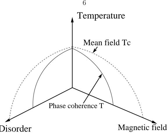
Temperature

Phase coherence T

Magnetic field

Disorder

Mean field Tc

Figure 1.1: Schematic phase diagram of disordered superconducting films. Disorder and magnetic field reduce the phase coherence temperature and eventually drive the system into insulating phase in which Cooper pairs are localized.

the vortices condense and dissipationless supercurrent is lost.

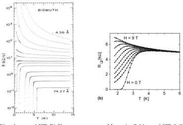
Disorder−tuned SIT, Bi film Magnetic−field−tuned SIT, InO film

Figure 1.2: Resistance vs. temperature traces in typical superconductor-insulator transition (SIT) experiments tuned by disorder (left, taken from Ref. [18] ) or per-pendicular magnetic field (right, taken from Ref. [19]).

fluctuations.

1.3

Vortex-boson duality

which is the low energy theory of the BCS theory or the Bogoliobov superfluid theory:

Z =

∫

Dθe−∫dxµL

L= 1

2ρs(∂µθ) 2

,

(1.16)

where ρs is the superfluid stiffness, θ is the phase of the superconductor/superfluid order parameter, and we set the phonon velocity to be 1 (for illustration purposes, we neglect the complication of non-linear dispersing phonons in superconducting films. See Chapter 3 for more details). Next, one introduces the current field jµ by a Hubbard-Stratonovich transformation:

Z =

∫

DθDjµe−

∫

dxµL

L= 1

2ρs

j_µ2+ ijµ∂µθ.

(1.17)

Then we split the phase field into a smooth part and a vortex part θ =θs+θv, and integrate out the smooth part to obtain the continuity constraint ∂µjµ= 0:

Z =

∫

DθvDjµδ(∂µjµ)e−

∫

dxµL

L= 1

2ρs

j_µ2 + ijµ∂µθv.

(1.18)

Now notice that the continuity constraint is automatically satisfied by introducing a gauge field αµ and parametrizing jµ as

jµ = 1 2πϵ

µνρ_∂

ναρ. (1.19)

Therefore upon integrating by parts, and noting the definition of vortex currents

j_µv = 1 2πϵ

µνρ_∂

the partition function now looks like

Z =

∫

DaµDjµve−

∫

dxµL

L= 1

8π2_ρ s

(ϵµνρ∂ναρ)2 −ijµvαµ.

(1.21)

This dual theory looks just like charges (which are vortices) interacting with a Maxwell gauge fieldαµ, and it contains all the physics of the original XY model. For example, phonon excitations in the original XY model now become photons with a Maxwell term; the well-known logarithmic interaction between vortices is represented as two-dimensional “Coulomb” interaction here if one integrates out α0 in the transverse gauge of αµ; the supercurrent now becomes the dual “electric field” (rotated by 90 degrees), while the boson density fluctuation becomes the dual “magnetic field”, which is easy to understand from (1.19); the Magnus force[43], which is the transverse force exerted by a supercurrent on a vortex, is simply recovered as the electric force in this dual formalism.

Interestingly, the Cooper pair supercurrent acts as the electric field for vortices, and the vortex current also acts as the electric field for Cooper pairs (AC Joseph-son effect[4]). Consequently the physical conductance is the inverse of the “vortex conductance”:

σphysical=

j E =

Evortex

jvortex

= 1

σvortex

. (1.22)

Due to this relation, a “vortex superfluid” (σvortex = 0) is an insulator (σphysical =

∞), and vice versa. Alternatively, this correspondence between the phases of the original XY model and those of the dual theory can be also understood by including an external electromagnetic field Aext,µ from the beginning and integrating out all fluctuating fields of both theories to show that in the superfluid phase of the original theory and in the “insulating phase” of the dual theory,

which gives a superfluid response

jµ =

∂L ∂Aext,µ

∼ρsAext,µ, (1.24)

while in the insulating phase of the original theory and in the “superfluid phase” of the dual theory

L ∼(ϵµνρ∂νAext,ρ)

2 _(1.25)

which is just the Maxwell theory giving an insulator response.

Since in disordered superconducting films, vortex mobility is µ ∼ e2ξ2/(~2σn) where σn is the normal state conductance, vortices are immobile in less disordered films[15, 14, 17]. Hence, the ground state is an insulating phase for vortices, i.e., physical superfluid phase. On the other hand, in strongly disordered films vortices are mobile, or when there is a strong external magnetic field which would be translated to a large background vortex density, the system is in a “Higgs” phase and vortices “condense”. This is an insulator where all excitations are gapped. That completes our discussion of the vortex picture for superconductor-insulator transitions.

1.4

Overview of our work on thin film

supercon-ductors

Motivated by the physics of superconductor-insulator transitions in thin-films, more experimental studies have been undertaken in recent years in several different direc-tions. One of them is to focus on the nature of the density of states (DOS) and the quasi-particle energy gap in superconducting thin films[44, 45, 46, 27, 30, 29, 32] and superconductor - normal-metal (SN) bilayers [47, 48, 49]. Interestingly, these studies found a broadening of the BCS peak and also a subgap density of states[45, 27, 30, 29, 32, 48]. Of particular interest to us is the work in Ref. [49], which studied a thin SN bilayer system, and found a surprisingly low value of the ratio of the energy gap to

InO film Ta film

Figure 1.3: The resistance vs. inverse of temperature (left) and resistance vs. tem-perature (right) in the metallic phase at intermediate values of magnetic field. Left: experiment on InO film, taken from Ref. [19]. Right: experiment on Ta film, taken from Ref. [53].

where it is claimed that the energy gap-Tc ratio should be bounded from below by

∼ 3.52. A drop below this bound, 2Eg/Tc < 3.52, was also observed in amorphous Bi films as it approaches the disorder tuned SIT[27, 30]. Similar trends were also observed in SN bilayers in Ref. [47] and in amorphous tin films in Ref. [46]. In Chapter 2, we show that a reduction of the 2Eg/Tc ratio in a dirty superconductor could be explained as a consequence of inhomogeneity in the pairing interaction.

Another direction of recent experimental studies is to investigate the films exhib-ing magnetic-field-tuned superconductor-insulator transition at lower temperatures (< 100mK) and higher magnetic fields (ranging from 1T to 15T). One puzzling ob-servation is that a metallic phase intervenes between the superconducting and the insulating phases[54, 55, 56, 35, 19, 57, 53, 58] (see FIG. 1.3). Near the “SIT critical point”, as temperature is lowered below∼100mK, the resistance curve starts to level off, indicating the existence of a novel metallic phase, with a distinct nonlinearI−V

resis-B

super−

metal(?)

conductor insulator unpairedstate

R

strange

Figure 1.4: A typical magnetoresistance curve of amorphous thin film superconduc-tors. As the magnetic field B increases, the superconducting phase is destroyed, and a possible metallic phase emerges. After which the system enters an insulating phase, where the magnetoresistance reaches its peak. The resistance drops down and approaches normal state value as B is further increased.

tance, as shown in FIG. 1.4. In Ta and MoGe films, as well as some InO films, the resistance peak is not as large, but is still apparent[54, 55, 56, 19, 57, 53].

Two competing paradigms may account for the metallic phase as well as the giant magnetoresistance. On one hand, the quantum vortex pictures [21, 40, 61, 62] attempt to explain these phenomena by extending the original simple superconductor-insulator transition theory as we dicussed in Sec. 1.3. The insulating phase at the peak of the magnetoresistance implies the condensation of quantum vortices as before, but to explain the high field negative magnetoresistance, one needs to explicitly incorporate unpaired electrons into the model and interpret the negative magnetoresistance as the gradual depairing of Cooper pairs and the appearance of a finite electronic density of states at the Fermi level. The intervening metallic phase is described as a delocalzed but yet uncondensed diffusive vortex liquid as described in Ref. [62]. In this picture disorder and charging effects are most important on length scales smaller or of order

ξ (the superconducting coherence length, typically of order 10nm).

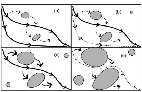
pic-Figure 1.5: Schematic representation of the percolation theory explanantion to the negative magnetoresistance in magnetic-field-tuned superconductor-insulator transi-tions. Taken from Ref. [63].

ture in Ref. [63] which phenomenologically captures both a metallic phase as well as the strongly insulating phase by assuming superconducting islands exhibit a Coulomb blockade for electrons. This theory also assumes that the major effect of the mag-netic field is to decrease the portion of superconducting puddles. This way the peak in the magnetoresistance arises from electron transport through the percolating nor-mal regions consisting of narrow conduction channels. To be more specific (see FIG. 1.5), when the magnetic field is large, superconducting islands are small, charging gap is large for electrons, and therefore conduction is mainly through the normal metal region (FIG. 1.5a). When the magnetic field is slightly lowered (FIG. 1.5b), superconducting islands become larger, but the charging gap is still large enough to penalize electrons trying to enter superconducting islands; however the enlarged su-perconductors squeeze the conduction path in the normal metal region, and therefore the resistance increases with decreasing magnetic field. When the magnetic field is further lowered (FIG. 1.5c,d), superconducting islands are finally large enough so that tunneling into them becomes energetically favorable, and the resistance is decreased with smaller magnetic fields. Finally, when superconducting islands percolate, the system enters the superconducting phase.

superconductor-metal transition using a phase glass model [68, 69] (see, however, Ref. [70] which argues against these results), but does not address the full magnetoresistance curve. Qualitatively, both paradigms above are consistent with magnetoresistance obser-vations, and recent tilted field[71], AC conductance[72], Nernst effect[73], and Scan-ning Tunneling Spectroscopic[74] measurements cannot distinguish between them. Particularly intriguing is the origin of the metallic phase - is it vortex driven or does it occur due to electronic conduction channels dominating transport through the film? In Chapter 3, we propose a new type of experiments, namely the drag resistance mea-surement, as a method capable to point to the correct theoretical picture.

1.5

From superconductivity to quantum Hall

ef-fect

The classical Hall effect, discovered more than a century ago, is straightforward to understand with classical electromagnetism. When charge carriers move in a per-pendicular magnetic field, charge will accumulate in the transverse direction which generates an electric field to balance the Lorentz force exerted by the perpendicular magnetic field. The Hall resistance, namely the transverse voltage drop divided by the longitudinal electric current, is therefore proportional to the magnetic field.

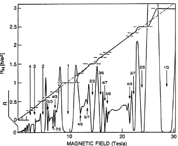
For two-dimensional electron gas (2DEG) in semiconductor heterostructures and later in graphene, when a strong perpendicular magnetic field commensurate with the electron density is applied, a series of remarkable quantum Hall states emerge[76, 77, 78]. What makes these states different from the classical Hall effect is the existence of plateaus in Hall resistance and the simultaneous vanishing of longitudinal resistance near certain integer and fractional filling factors (defined as ν ≡ ρ/(B/ϕ0), ρ is the carrier density, B is the magnetic field, ϕ0 is the flux quantum). When the filling factor slightly deviates from these special values, the Hall resistance stays quantized atRxy = 1_νeh2 (see FIG. 1.6).

Figure 1.6: Experimental results of the Hall resistance and the longitudinal resistance in 2DEG. Taken from Ref. [75].

electrons by invoking quenched disorder. Disorder is necessary for the existence of this plateau, which can be understood either through a Galilean invariance argument[79] or a vortex argument (see below). For fractional quantum Hall effect, the Coulomb interaction plays a crucial role[79, 80, 81] instead. The fractional quantum Hall ef-fect with odd-integer-denominator filling factor can be understood with Laughlin’s wavefunctions[82], and Chern-Simons flux attachment approaches including compos-ite boson[83, 84] and composcompos-ite fermion approaches[85, 86]. Both integer and frac-tional quantum Hall effect have a gap for all bulk excitations, but it has been shown that gapless chiral excitaions exist on the edge[81]. In recent years, a lot of interest have been generated by the possibility of non-abelian quantum Hall states in higher Landau levels and their possible applications to topological quantum computations[87, 88].

To lay down the foundation for later sections, we now focus on Laughlin states at

answer is[82]

ψ =∏ i<j

(zi−zj)2k+1exp

[

−∑

i

|zi|2/(4l2)

]

, (1.26)

wherelis the magnetic length, andzj =xj+ iyj. This wavefunction has almost unity overlap with the exact ground state, and its virtue could be understood by the fact that it has no wasted zeros[89, 80], which means the following. Given N electrons and therefore N(2k+ 1) flux quanta, when we view the Langhlin wavefunction as a wavefunction ofz1 and take this electron around the sample in a loop, the wavefunc-tion should pick up a Aharonov-Bohm phase 2πN(2k+ 1), which implies that there have to be N(2k+ 1) zeros in the wavefunction. Among these zeros, Pauli-exclusion principle only requires N of them to lie on other electrons, however in the Laughlin wavefunction all zeros do lie on other electrons, which is very efficient in keeping electrons apart and lowering the interaction energy.

Next, we proceed to discuss the composite boson theory which carries the features of quantum Hall states in a very compact way. From the Laughlin wave function, we see that in terms of Berry’s phase, essentially electrons see each other as a 2π(2k+ 1) flux source, in this way they are kept apart and the interaction energy is lowered. In the same spirit, we can trade each electron for 2k+ 1 flux quanta and a composite boson, and transform the original Lagrangian for electron ψ

L=ψ†(i∂t−At)ψ+ 1 2mψ

†(_{−i∇ −A}⃗

ext

)2

ψ+V(|ψ|), (1.27) where V is the potential energy including the Coulomb interaction and disorder po-tentials, into the Lagrangian for composite boson ϕ and a Chern-Simons gauge field

aµ:

L=ϕ†(i∂t−at−At)ϕ+ 1 2mϕ

†(_{−i∇ −⃗a−A}⃗

ext

)2

ϕ+V(|ϕ|) + 1

4π(2k+ 1)aµϵ µνρ_∂

respect to at, which leads to

(2k+ 1)ϕ†ϕ = 1

2π∇ ×⃗a. (1.29)

Therefore at the mean-field level, the Chern-Simons flux and the external magnetic field cancel each other, and composite bosons see zero net flux. As bosons, they condense and form a superfluid. Since the total electric field vanishes inside a charged superfluid, we have

⃗

e+E⃗ext= 0, (1.30)

where the “electric field” ⃗e ≡ −∂t⃗a− ∇at. Minimizing the action with respect to ⃗a, we obtain

(2k+ 1)⃗j = 1

2πzˆ×⃗e, (1.31)

and hence the defining property of quantum Hall effect

⃗j = 1

2π(2k+ 1)

⃗

Eext×zˆat filling fraction ν = 1 2k+ 1.

Therefore, the quantum Hall effect at filling factor ν = 1/(2k + 1), the so-called Laughlin fraction, can be understood as a condensate of composite bosons which is formed by attaching (2k+ 1) flux quanta to each electron, and these background fluxes cancel the external magnetic field exactly at these special filling factors. Vortex excitations of this composite boson superfluid are introduced when the filling fraction is slightly moved away fromν = 1/(2k+ 1), but similar to the situation of supercon-ductors, vortices will be pinned by quenched disorder, and the conductance remains the same. This explains the Hall plateau. One can also generalize the vortex-boson duality formalism to transform the above Lagrangian to reveal the vortex degrees of freedom explicitly and show that they have fractional charge and statistics. In the low-energy long-wavelength limit, denoting θ the phase of the composite boson, we have

L = 1

2ρ(∂µθ−A ext

µ −aµ)2+

1

4π(2k+ 1)aµϵ µνρ_∂

Next, one introduces the composite-boson current field jµ through the Hubbard-Stratonovich transformation:

L = 1

2ρj

2 µ+ ijµ

(

∂µθ−Aext_µ −aµ

)

+ 1

4π(2k+ 1)aµϵ µνρ_∂

νaρ. (1.33)

Again, we split the phase field into a smooth part and a vortex part θ =θs+θv, and integrate out the smooth part to obtain the continuity constraint ∂µjµ = 0 which is solved by introducing a gauge field jµ= ₂1_πϵµνρ∂ναρ :

L = 1

8π2_ρ(ϵ µνρ_∂

ναρ)2 + i 1 2πϵ

µνρ_∂ ναρ

(

∂µθv−Aextµ −aµ

)

+ 1

4π(2k+ 1)aµϵ µνρ_∂

νaρ. (1.34) Integrating by parts, noting the definition of vortex currents jv

µ= 1 2πϵ

µνρ_∂

ν∂ρθv, and integrating out the Chern-Simons field aµ, we can rewrite the Lagrangian into the following form:

L = 1

8π2_ρ(ϵ µνρ_∂

ναρ)2 +

(2k+ 1) 4π αµϵ

µνρ_∂

ναρ−i 1 2πϵ

µνρ_∂

ναρAextµ −ijµvαµ. (1.35)

Unlike the case of superconductors, the gauge field αµ which represents the (compos-ite) boson density fluctuation now acquires a Chern-Simons term, which renders it a gap. Therefore the quantum Hall fluid is incompressible at ν = 1/(2k+ 1), while superfluid and (1D,2D) superconductors are compressible. The Chern-Simons term for αµ also indicates that 1/(2k+ 1) flux quantum is attached to each vortex, which explains their fractional statistics. According to the third term in this Lagrangian,

Aext_t is coupled to the one flux quantum of αµ, which means one flux quantum of αµ has one unit of electric charge. Since each vortex has 1/(2k+ 1) flux quantum, each of them has 1/(2k+ 1) electric charge as well. When vortices are absent, one can also integrate out all fluctuating fields and obtain

L= 1

4π(2k+ 1)A ext µ ϵ

µνρ

which gives

jµ= δL

δAext µ

= 1

2π(2k+ 1)ϵ µνρ_∂

νAextρ , (1.37) which is again the defining property of the quantum Hall effect at ν = 1/(2k+ 1).

1.6

Bilayer quantum Hall effect: a hidden

super-fluid

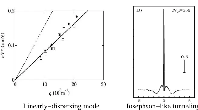
In bilayer two-dimensional electron systems with negligible interlayer tunneling and total filling factorνtot = 1, when the layer separationdis comparable to the magnetic length l, a remarkable bilayer quantum Hall state with interlayer phase coherence emerges due to the interlayer Coulomb interaction[90]. The extra layer index degrees of freedom adds a lot of interesting physics to the system, and many remarkable experimental signatures of this phase predicted by theories have been observed in experiments, including enormous enhancement of zero bias interlayer tunneling[91], linearly dispersing Goldstone mode[92], quantized Hall drag[93], and vanishing resis-tance in counterflow[94].

There are several equivalent and complimentary ways to understand this bilayer quantum Hall state. In the pseudospin ferromagnet approach[95], one treats the layer index as pseudospin, and by Hund’s rule, the ground state is a pseudospin ferromagnet which makes the spatial wavefunction completely anti-symmetric and therefore lowers the interaction energy. In addition, due to the charging energy at nonzero layer separation, the SU(2) symmetry is broken down to the easy-plane U(1) symmetry, and the ground state has a pseudospin lies in the xy-plane. Denoting ψ1,X andψ2,X the electron field operators at guiding centerXin the two layers respectively, we have

and the ground state can be written as

|Ground State⟩ ∼∏ X

(

ψ₁†_,X+eiθψ₂†_,X

)

|0⟩. _(1.39)

These are what we meant by interlayer phase coherence. Note its remarkable conse-quence: each electron wavefunction is a coherent superposition of the state in each layer, even though we start with no interlayer tunneling! In addition, since at each guiding center there is only one electron, we have avoided paying for the strong inter-layer Coulomb repulsion, which is partly the reason why this state has a low energy. Also note that the ground state wavefunction (1.39) can be written in a BCS form (cf. Eqn. 1.5)

|Ground State⟩ ∼∏ X

(

1 +eiθψ†_2,Xψ1,X

)

|G⟩, where |G⟩ ∼∏

X

ψ₁†_,X|0⟩. _(1.40)

but in experiments dissipationless counterflow is only seen in the zero-temperature limit[94]. The effect of quenched disorder is believed to be crucial to reconcile these discrepancies[97, 98, 99], although a quantitative understanding is still lacking. Us-ing the pseudospin analogy, one can also deduce the actions for various excitations including spin waves, skyrmions, merons, etc., and estimate the parameters in these effective actions using microscopic parameters[95].

Next, we briefly introduce the composite boson formalism[96, 95], which gives the same results in an elegant way. The basic physical picture is the same as those in the pseudospin ferromagnet picture and the exciton condensate picture: since the interlayer distance between electrons d is comparable to the intralayer distance (∼ magnetic length l), both interlayer and intralayer Coulomb interactions are strong, and electrons tend to get as far as possible from other electrons both in the same layer and in the other layer. Now we formulate this idea by following the previous section’s idea that when electrons avoid each other, they see each other as an odd integer number of flux quanta. Here, because of the total filling factor νtot = 1 and because the strong interlayer interaction, each electron see those both in their own layer and those in the other layer as 2π flux source (equivalently, one zero in their wavefunction). Thus, each electron is traded for one composite boson and one flux quantum, and this background flux cancels the external magnetic field due to the total filling factor νtot = 1. Generalizing the formalism of the previous section, in the low-energy long-wavelength limit, the Lagrangian for composite bosons is

L= 1

2ρ(∂µθ1−aµ−A ext µ )

2₊1

2ρ(∂µθ2−aµ−A ext µ )

2₊ 1 4πaµϵ

µνρ_∂

νaρ, (1.41)

where θ1,2 are the phases of the composite boson fields of each layer due to the flux attachment transformation. Performing the same duality transformation as in the previous section, and defining

Josephson−like tunneling Linearly−dispersing mode

Figure 1.7: Experimental evidence of the interlayer coherent bilayer quantum Hall state at ν = 1. Left: excitation energy vs. wavevector - evidence for a linearly-dispersing Goldstone mode. Taken from Ref. [92]. Right: interlayer tunneling con-ductance vs. bias voltage - evidence for the Josephson-like interlayer tunneling. Taken from Ref. [91].

where α1,2 and j1,2 are the gauge fields introduced in the duality transformation and the composite boson currents in the two layers, respectively, we can rewrite the Lagrangian as

L =L++L−,

L+ = 1 16π2_ρ(ϵ

µνρ_∂

να+ρ)2+ 1 4πα+µϵ

µνρ_∂

να+ρ−i 1 2πϵ

µνρ_∂

να+ρAextµ ;

L− = ₁₆1_π2_ρ(ϵ µνρ_∂

να−ρ)2

(1.43)

when vortices are absent. Apparently, the transport property of the “+” sector corresponds to treating the bilayer system as a whole. In this sector, one can neglect the less relevant Maxwell term and integrate out the fluctuating gauge field αµ to obtain

L+ = 1 4πA

ext µ ϵ

µνρ

∂νAextρ , (1.44) which is again the defining property of a ν= 1 quantum Hall state.

this state is that its “-” sector has no Chern-Simons term! It looks exactly the same as the dual representation of a superfluid [cf. Eqn. (1.21)]. Immediately this leads to the prediction of dissipationless counterflow, a linearly dispersing mode which is rep-resented as “photons” here, and the analog of Josephson tunneling, as we discussed earlier.

1.7

Half-filled Landau level: a hidden Fermi liquid

This interlayer coherent quantum Hall state only survives when the ratio of layer separation d and the magnetic length l is relatively small. In the opposite limit

d/l → ∞, two layers are decoupled, and each layer is at half-filling. Surprisingly, a half-filled Landau level behaves as a Fermi liquid, and much progress has been made in understanding this “composite fermion” Fermi liquid phase using the Chern-Simons approach[100, 101, 102, 103, 104] and the dipolar quasiparticle approach[105, 106, 107, 108, 109, 80].

The basic idea for this composite fermion Fermi liquid phase is quite simple to illustrate using flux attachment. At half-filling, if we try to trade electrons for com-posite particles and flux quanta to cancel the background flux as we did in previous sections, we have to attach two flux quanta to each electron. Therefore when two electrons are interchanged, we obtain an additional 2π phase instead of a π phase for Laughlin states or bilayer νtot = 1 state. Hence, what we have obtained are com-posite fermions instead of comcom-posite bosons. Consequently, electrons at half-filling is equivalent to composite fermions with no magnetic field, which is naturally in a Fermi liquid state. However, due to the strong coupling of composite fermions with fluctuat-ing Chern-Simons gauge fields, the composite Fermi liquid is much more complicated than conventional ones.

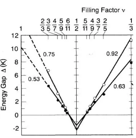
Figure 1.8: Activation gap of quantum Hall statesν =p/(2p+ 1) as a function of the filling factor ν, measured in Ref. [110]. The linear relation supports the composite fermion picture, and the slope is inversely proportional to the composite fermion mass.

easy to see that (~=e= 1):

∆B ≡B−B1/2 = 2π

ρ

p, with B1/2 ≡4πρ, (1.45)

where ρ is the electron density. Thus, the composite fermions are in an integer quantum Hall state withpLandau levels filled. In other words, the fractional quantum Hall effect at ν = p/(2p+ 1) can be understood as integer quantum Hall effect of composite fermions, and the activation gap in these states can be identified as the cyclotron gap of composite fermions:

Eg = ∆B

m_∗ =

2πρ

pm_∗, (1.46)

m_∗ being the composite fermion mass, which can be determined by fitting measured gap values near ν = 1/2. Experiments have indeed confirmed the linear relation between the gap Eg and ∆B (see FIG. 1.8), which gives strong support for the composite fermion picture.

in half-filled Landau levels, and typically there are at least qualitative agreements with composite fermion theories, although it is often difficult to find very good quantita-tive agreements (see review articles by Refs. [111, 104, 80]). These efforts include measuring surface-acoustic-wave velocity shift[111], cyclotron orbit radius[112, 113], NMR relaxation rate T₁−1[114], specific heat which is expected to be linear in T but with logarithmic corrections[115], Coulomb drag resistance which is expected to scale as T4/3_{[116], etc.}

1.8

Overview of our work on bilayer quantum Hall

systems

Although we understand well both the coherent phase at d/l→0 and the composite Fermi liquid state at d/l → ∞, the transition between them has been shrouded in mystery. There have been many experimental[117, 118, 119, 120, 121, 122, 123, 124, 125, 126, 127, 128, 129, 130] and theoretical[131, 132, 133, 134, 135, 136, 137, 138, 139, 140, 141, 142, 143] studies regarding the nature of this transition. While some of these theoretical works point to a direct transition between the two limiting phases, either continuous[140] or of first order[137, 138], some other works predict the existence of various types of exotic intermediate phases, including translational symmetry broken phase[131, 132, 133, 141], composite fermion paired state[134, 135, 142], phase of coexisting composite fermions and composite bosons[139, 143, 144], and quantum disordered phases[136], etc.

indicate that at least one of the phases involved in the transition is not fully polarized, and that the polarization changes significantly across the transition. The most likely possibility is that the incoherent composite Fermi liquid phase at large d/l is only partially polarized, as shown by other experiments on single layer atν = 1/2[114, 145]. If the transition between the coherent phase and the less polarized incoherent phase is a thermodynamic phase transition, it must be of first order: The magnetization is discontinuous across the transition, and, as the experiments of Ref. [121] found, the transition can be tuned using a Zeeman field which is conjugate to the magnetization. These two facts together imply the first order nature of the transition. An alternative to the thermodynamic transition scenario is a singularity-free quantum crossover as was suggested recently in Refs. [142, 143].

In Chapter 4, we assume that the transition tuned by d/l is a thermodynamic first-order transition between spin-polarized coherentνtot = 1 quantum Hall state and partially-polarized composite Fermi liquid state, and derive the Clausius-Clapeyron relations for this system. The Clausius-Clapeyron relations will allow us to obtain the phase boundary shapes for the transition; a comparison of these boundaries with experiments presents a stringent consistency test of the first order transition scenario.

1.9

One-dimensional random hopping model

In this section, we switch from two-dimensional systems to one-dimensional cases. Being particularly interesting to us is the one-dimensional non-interacting random hopping model, namely tight-binding model with off-diagonal disorder:

H =−∑ n

Jnc†ncn+1+h.c., (1.47)

Ising chains in transverse field, and random mass Dirac fermions. This model exhibits many surprising features. Early theoretical works[146, 147, 148, 149] focus on prop-erties derivable from the mean local Green’s function, notably the typical localization length and the mean density of states. For example, the state with zero energy is a delocalized state[148]. To illustrate this, we start with the Schrodinger equation of this system

−Jnψn+1−Jn−1ψn−1 =Eψn, (1.48) where ψn is the wavefunction at site n. For zero energy, this equation gives

ψn+1

ψn−1

=−Jn−1

Jn

. (1.49)

Thus,

ψ2n+1

ψ1 =

(

−J2n−1

J2n

) (

−J2n−3

J2n−2

)

...

(

−J1

J2

)

. (1.50)

Using the definition of localization lengthλ [147] 1

λ =−nlim→∞ 1 2nln

ψ2n+1

ψ1

(1.51)

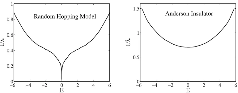
and the central limit theorem, one readily sees that the inverse of the localization length vanishes. Therefore this state has infinite localization length. More detailed analysis[149] shows that the localization length diverges as ∼ ln|E| near the band-center, and the mean density of states (DOS) also diverges as ∼ 1/|E(lnE2₎3| _as energy E approaches band-center. These behaviors are very different from Anderson insulators in which case disorder comes into diagonal terms and there are no singu-larities in the spectrum of the localization length or the density of states (see FIG. 1.9).

in-−60 −4 −2 0 2 4 6 0.2

0.4 0.6 0.8 1

E

1/

λ

Random Hopping Model

−60 −4 −2 0 2 4 6 0.5

1 1.5

E

1/

λ

Anderson Insulator

Figure 1.9: Comparison of the inverse of the localization length vs. energy in (left) random hopping model and (right) Anderson insulator.

teracting fermion and boson systems have also been investigated. In fermion case[152], it has been shown that random hopping amplitude could lead to a novel type of in-stability; in boson case[153, 154], novel “Mott glass” phase has been predicted in addition to usual Mott insulating and superfluid phases.

Nevertheless, pure random hopping model behavior is extremely difficult to engi-neer experimentally. This is mainly because diagonal disorder inevitably comes in, and any amount of diagonal disorder would break the particle-hole symmetry of the random hopping model and thereby destroy the interesting properties near the band-center. Hence, it is highly desirable to find a feasible and robust way to experimentally realize a random hopping model.

1.10

Realizing random hopping model with

dy-namical localization

163, 164, 165, 166, 167, 168, 169]. The basic idea of Dynamical Localization is the following. Consider a double well with a tunneling amplitude J/2 and a potential energy difference oscillating at frequency ω:

H=−J 2(a

†_b+b†_{a) +} V

2 cos(ωt)(a

†_a−b†_{b). (1.52)}

Switching to spin representation

Sx = 1 2(a

†_b+b†_{a), S} z =

1 2(a

†_a−b†_{b), (1.53)}

we have

H =−J Sx+V cos(ωt)Sz. (1.54) By performing a unitary transformation with

ψ =Uψ,˜ U =e−iVωsin(ωt)Sz, (1.55)

one transforms the original Schrodinger equation i∂tψ =Hψ into

i∂tψ˜=Hef fψ,˜ (1.56)

where

Hef f =U†HU −U†(i∂tU) =−J eiVωsin(ωt)SzS_xe−i

V

ωsin(ωt)Sz

=−J

[

Sxcos

(

V

ω sinωt

)

−Sysin

(

V

ω sinωt

)]

,

(1.57)

which can be expanded as a series of Bessel functions. In the limit of fast oscillation, the leading order term is

Hef f ≈ −JJ0

(

V ω

)

Sx =−

J

2J0

(

V ω

)

Chapter 2

Effect of Inhomogeneous Coupling

On BCS Superconductors

2.1

Introduction

As discussed in Chapter 1, motivated by the thin-film physics, the experimental work in Ref. [49] studied a thin SN bilayer system, and found a surprisingly low value of the ratio of the energy gap to Tc, in contradiction to standard BCS theory, and the theory of proximity [50, 51, 52] where it is claimed that the energy gap-Tcratio should be bounded from below by ∼ 3.52. A drop below this bound, 2Eg/Tc < 3.52, was also observed in amorphous Bi films as it approaches the disorder tuned SIT [27, 30]. Similar trends were also observed in SN bilayers in Ref. [47] and in amorphous tin films in Ref. [46].

In this Chapter we show that a reduction of the 2Eg/Tc ratio in a dirty supercon-ductor could be explained as a consequence of inhomogeneity in the pairing interac-tion. In SN bilayer thin films, thickness fluctuations of either layer result in effective pairing inhomogeneity (in thin SN bilayers the effective pairing is the volume averaged one, c.f., Ref. [51, 52] and Sec. 2.4). Such inhomogeneities in other systems occur due to grain boundaries, dislocations, or compositional heterogeneity in alloys[170]. For simplicity we will assume in our analysis that the pairing coupling constant takes a one-dimensional modulating form:

In bilayer SN films, the effect of localization and Coulomb interaction is minor compared to proximity effect, and therefore we will neglect these complications in this chapter.

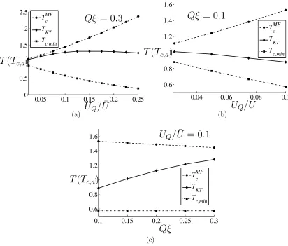
In our results, the ratio between the inhomogeneity length, L ≡ 1/Q, and the superconducting coherence length ξ, plays a crucial role. When Qξ ≫ 1, the super-conducting properties are determined by an effective coupling ¯U . Uef f < U¯ +UQ [171]. In this limit, the ratio 2Eg/Tc is preserved at the standard BCS value ∼3.52. Small corrections are obtained when 1/(Qξ) is finite. In the opposite limit, Qξ≪1, the system tends to be determined by the local value ofU(x). Within mean field the-ory, the ratio 2Eg/Tc is generally suppressed from the BCS value 3.52; in 2d, however, when one includes the thermal phase fluctuation and studies the Kosterlitz-Thouless temperature,TKT, the ratio 2Eg/TKT can be larger than the usual BCS value. These results on 2Eg/Tc are summarized in FIG. 2.6.

Our analysis is inspired by similar previously studied models. Particularly, theTc of the clean case of this model has been analyzed in Ref. [171]. Here we extend the study of non-uniform pairing to bothTc and zero-temperature properties of disordered films, in the regime where the electron mean free path l obeys 1/kF ≪l≪ξ0 ∼ ~_Tv_cF, which is relevant to the experiments of Long et al.[48, 49]. Note that while Anderson theorem states that the critical temperature and gap of a homogenous superconductor do not depend on disorder[10], in an inhomogeneous system the theorem does not hold. Indeed, we find that the results of Ref. [171], are modified in the dirty case. In another related work, a system with a Gaussian distribution of the inverse pairing interaction was studied [172, 173]. It was shown that an exponentially decaying subgap density of states appears due to mesoscopic fluctuations which lie beyond the mean field picture. Finally, inhomogeneous coupling in the attractive Hubbard model [174, 175] and lattice XY model [176] were also analyzed, with relevance to High-Tc materials.

with spatially uniform coupling constant. Then, in Sec. 2.3 we discuss the cases with nonuniform coupling classified by the competition of two length scales: the coherence length ξ and the length scale associated with the variation of the coupling constant

L= 1/Q. We will also discuss the effect of other types of inhomogeneities briefly. In section 2.4 we provide a useful analogy with superconductor-normal metal superlattice to provide more physical intuition about our results on the energy gaps. In section 2.5 we will summarize our analysis and discuss the connection with experimental results.

2.2

The gap equation of a nonuniform film

The starting point of our analysis is the standard s-wave BCS Hamiltonian:

H = H0+Hint+Himp,

H0 =

∑

σ

ψ†_σ(⃗r) ˆξψ(⃗r)σ,

Hint = −U(⃗r)ψ_↓†(⃗r)ψ_↑†(⃗r)ψ↑(⃗r)ψ↓(⃗r), (2.2)

where ˆξ ≡ −∇_2m2 −µ, and U(⃗r)> 0 is the attractive coupling constant between elec-trons, and Himp includes scattering with nonmagnetic impurities. When the pairing interaction,U(⃗r), is nonuniform, so is the order parameter in this system. A standard technique to tackle this non-uniform superconductivity problem is the quasiclassical Green’s functions [178, 12, 179]. In the dirty limit ℓ ≪ ξ0 ∼ ~_Tv_cF, the quasiclassical Green’s functions obey a simple form of the Usadel equation, which in the absence of a phase gradient is:

D

2

(

−∇2_θ)_{= ∆ cosθ−ω}

nsinθ, (2.3)

where D = 1

Green functions g and f:

g = cosθ, f =f†=−isinθ. (2.4)

Also, we list the relation between the integrated quasiclassical Green’s function and Gor’kov’s Green’s function Gand F:

g(⃗r) =

∫

dΩp 4π

∫

dξp

iπ G(⃗r, ⃗p) =

1

iπNF

∫

d3p

(2π)3G(⃗r, ⃗p),

f(⃗r) =

∫

dΩp 4π

∫

dξp

iπ F(⃗r, ⃗p) =

1

iπNF

∫

d3_p

(2π)3F(⃗r, ⃗p),

where ⃗r is the center of mass coordinate, and ⃗p is momentum corresponding to the relative coordinate; Ωp is the angle of momentum ⃗p and NF is the density of states (per spin) of the normal state at the Fermi energy. The self-consistency equation reads:

∆(⃗r) =U(⃗r)NFπT

∑

n

ifωn(⃗r). (2.5)

For simplicity we assume the pairing is as given in Eq. (2.1),

U(⃗r) = ¯U +UQcos(Qx).

2.2.1

The uniform pairing case

Before analyzing the inhomogeneous pairing problem, let us briefly review the calcu-lation ofTc, the superconducting order parameter ∆(T = 0), and the DOSν(E) of a dirty superconductor with a spatially uniform coupling constant U, using quasiclas-sical Green’s functions. In this case Eqs. (2.3) and (2.5) admit a uniform solution for bothθ and ∆:

θ = arctan

(

∆

ωn

)

Using (2.5), we obtain the standard BCS self-consistency equation:

1 = U NFπT

∑

n

1

√

∆2_+ω2 n

. (2.7)

Tc and ∆(T = 0) are easily obtained from (2.7):

Tc = 2C

π ωDe

− 1

U NF_{,∆(T=0) = 2ωDe}−

1

U NF_.

where C = eγ ≈ 1.78, with γ = 0.5772. . . the Euler constant, and ωD the Debye frequency. The DOS can be obtained from the retarded quasiclassical Green’s func-tion: ν(E) = Re{gR(E)}, which can be obtained from g(ωn) = cos(θn) by analytical continuationiω →E+i0+_:

ν(E) = Re√ −iE

∆2−_(E+i0+₎2 =

  

E √

E2_−∆2, if E >∆ 0, if E <∆

.

Thus there exists a gap in the excitation spectrum Eg = ∆, and its ratio withTc is a universal number π/C ≈ 1.76. As expected, these results for dirty superconductors are exactly the same as those of clean superconductors, thus explicitly illustrating Anderson theorem.

2.3

The case of inhomogeneous pairing

Using the formalism reviewed in the previous section, we now discuss the non-uniform superconducting film. Our discussion will concentrate on the limits of fast and slow pairing modulations, i.e., large and small Qξ respectively (ξ is the zero temperature coherence length in the dirty limit: ξ = √~D/∆¯T=0 ∼

√

2.3.1

Fast pairing modulation: proximity enhanced

super-conductivity

With a nonuniform coupling U(x), uniform solution of either θ(x) or ∆(x) no longer exists. When fast pairing modulation are present, the angle θ is dominated by its

k = 0 Fourier component, θ0, since it can not respond faster than its characteristic length scaleξ. Corrections to the uniform solution are of the formθ1cos(Qx), and are suppressed by powers of _Qξ1 . From Eq. (2.5), we see that in contrast to θ, the order parameter ∆(x) has a factor of U(x) in its definition, and therefore it can fluctuate with the fast modulation of U(x). The modulating component of ∆(x) is thus only suppressed by UQ/U¯, while the modulating part of θ(x) is suppressed by bothUQ/U¯ and 1/(Qξ). Keeping both 1/Qξ ≪1 and expanding inUQ/U¯, we can perturbatively solve Eqs. (2.3) and (2.5). Starting with:

∆(x) = ∆0+ ∆1cos(Qx), θ(x) = θ0+θ1cos(Qx); (2.8)

Eq. (2.3) can be solved order by order:

θ0 = arctan

(

∆0

ωn

)

, (2.9)

θ1 = ∆1

ωn D

2Q 2√_ω2

n+ ∆20+ωn2 + ∆20

.

The self-consistency equation (2.5) can be Fourier transformed:

∆0 = NFπT

∑

ωn

(

¯

Usinθ0 + 2

UQ 2

cosθ0 2 θ1

)

, (2.10)

∆1

2 = NFπT

∑

ωn

(

¯

Ucosθ0

2 θ1+

UQ 2 sinθ0

)

,

where the ωn index of θ0 and θ1 is implicit.

When T →Tc, we can linearizeθ0 andθ1 with respect to ∆0 and ∆1, respectively:

sinθ0 ≈ ∆0

|ωn|

, θ1(cosθ0)≈

∆1

|ωn|+DQ 2 2

Note that

N0

∑

n=0 1

n+ 1/2 ≈lnN0+ 2 ln 2 +γ for N0 ≫1, (2.11) where γ is the Euler constant, we have approximately

2πT ωD

2πT

∑

ωn=0

1

ωn

≈ ln(2CωD/πT), (2.12)

2πT ωD

2πT

∑

ωn=0

1

ωn+DQ2/2

≈ ln

(

1 + ωD

DQ2_/2

)

,

where, as before, C =eγ _{≈1.78 andω}

D is the Debye frequency. Defining

K0 = ¯U NF ln(2CωD/πT), K1 = ¯U NFln

(

1 + 2ωD

DQ2

)

, (2.13)

we get

∆0 = K0∆0 + 1 2

UQ ¯

U K1∆1,

∆1 =

UQ ¯

U K0∆0+K1∆1.

Tc is the temperature at which this equation admits a nonzero solution:

Tc = 2C

π ωDexp

(

− 1

Uef fNF

)

, (2.14)

where the effective pairing strength is:

Uef f = ¯U

( 1 + ( UQ ¯ U )2 K1 2(1−K1)

)

. (2.15)

This is the dirty case analogue of the result obtained by Ref. [171].

equations (2.10) become integrals, which can be performed (see also Appendix 2.A):

∆0 =NFU¯∆0ln

(

2ωD ∆0

)

+1 2

UQ ¯

U K1∆1,

∆1 2 =

K1∆1

2 +

NFUQ 2 ∆0ln

(

2ωD ∆0

)

, (2.16)

thus giving the solution

∆0(T=0) = 2ωDexp

(

− 1

Uef fNF

)

,

∆1(T=0) = ∆0(T=0)

UQ

Uef f 1 1−K1

.

with the sameUef f defined in (2.15). Noting that ∆0 is the spatially averaged value of the order parameter ¯∆, we arrive at the conclusion that in the limit Qξ ≫ 1, the ratio

2 ¯∆

Tc

= 2∆0(T=0)

Tc

= 2π

C (2.17)

is preserved.

The modification of the gap, however, must be addressed separately. Although the gap and the order parameter coincide for a uniform BCS superconductor, this is not generally true in a nonuniform superconductor. To obtain the DOS and the gap one has to rephrase the problem in a real-time formalism and calculate the retarded Green’s function which is parameterized by a complex θ(x, E) =θ′(x, E) +iθ′′(x, E) with both θ′, θ′′ real, and then compute the DOS via ν(x, E) = RegR_{(x, E) =} Re cosθ(x, E) = cosθ′coshθ′′[12, 179]. Naively one can perform the prescription

4 6 8 10 0.95

0.96 0.97 0.98 0.99 1

∆

1=0.1∆0

∆

1=0.2∆0

E

(∆

)

Qξ

Figure 2.1: The energy gap,Eg, measured in units of ∆0, vs. QξforQξ≫1. The two curves are for ∆1/∆0 = 0.1 and 0.2, respectively. Here, ∆0 and ∆1 are the uniform and oscillating components of the order parameter, respectively. Qis the modulating wavevector of the inhomogeneous coupling constant; ξ is the superconducting coher-ence length. The estimated numerical error of Eg/∆0 is about 0.01. The deviation of

Eg from ∆0 is small, but it increases with larger ∆1/∆0 or smaller Qξ.

In real time, Eq. (2.3) becomes:

−D

2∂ 2

xθ′ = cosθ′(∆ coshθ′′−Esinhθ′′),

D

2∂ 2

xθ′′ = sinθ′(∆ sinhθ′′−Ecoshθ′′). (2.18)

We numerically solved these coupled equations with periodic boundary condition on [0,2π/Q], and computed the DOS ν(E) = cosθ1coshθ2, and thereby obtained the gap. We find that despite the fluctuating ∆(x), the energy gap, Eg, is spatially uniform. Fig. 2.1 shows a graph ofEg vs. Qξ for ∆1/∆0 = 0.1 and 0.2. Again, in the plot we define the coherence lengthξto be√~D/∆¯T=0 =

√

~D/∆0,T=0. One can see that in the limit Qξ → ∞ Eg coincides with ∆0, and nonzero 1/(Qξ) brings about only small corrections to make the gap slightly smaller than ∆0. These corrections increase with smallerQξor largerUQ/U¯ (i.e., ∆1/∆0). Thus we find that for Qξ≫1 case

2Eg(T=0)

Tc

. 2∆0(T=0)

Tc

= 2π

It is easy to understand the uniformity ofEg, since the wave function of a quasiparticle excitation should be extended on a length scale 1/Q≪ξ. Some intuition for the fact that Eg ≈∆0 is provided in Sec. 2.4.

2.3.2

Slow pairing fluctuations: WKB-like local

supercon-ductivity

When the pairing strength fluctuates slowly, i.e., over a large distance, both the Green’s functions and the order parameter ∆(x) can vary on the length scale of 1/Q, and we can approximate the zeroth order solution by a ’local solution’:

θ0(x) = arctan

(

∆(x)

ωn

)

, (2.20)

where ∆(x) is to be solved from the self-consistency equation. This ’local’ property of the system implies a large spatial variation of both ∆(x) andθ(x), in contrast to the

Qξ ≫ 1 case. To improve the zeroth order solution, we write θ(x) = θ0(x) +θ1(x). Neglecting the small gradient term of θ1, one can solve for θ1 from Usadel’s equation (2.3) :

θ1 =

D

2

(

ωn∂x2∆ (∆2_+ω2

n)3/2

− 2∆ωn(∂x∆)2 (∆2_+ω2

n)5/2

)

, (2.21)

thus the self-consistency equation (2.5) becomes

∆(x) =U(x)NF2πT

ωD 2πT ∑ n=0 ( ∆ √

∆2_+ω2 n

+√ ωn ∆2_+ω2

n

θ1

)

. (2.22)

In the Ginzburg-Landau regime, one is justified in keeping lowest order terms in (2.22):

∆(x) = U(x)NF

{

∆(x) ln

(

2CωD

πT

)

− 7ζ(3)

8π2_T2∆ 3

(x) +π~D

8T ∂

2 x∆(x)

}

where ζ(n) is the Riemann ζ function. Remarkably, equation (2.23) is nothing but the Ginzburg-Landau equation for a modulating coupling constant U(x) with Qξ≪

1, and is precisely the dirty case analogue of equation (9) in Ref. [171], with ξ

replaced by the dirty limit expression ˜ξ2 = ~πD/8T ( ˜ξ is slightly different from the coherence length defined in this work ξ ≡ √~D/∆¯T=0, where ¯∆ is the spatially averaged ∆(x)). In the limit <