Identification of cement manufacturing raw materials using machine vision

(1)

University of Southern Queensland

Faculty of Health, Engineering and Sciences

Identification of Cement Manufacturing

Raw Materials Using Machine Vision

A dissertation submitted by

Lindsay Notley

In fulfilment of the requirements of

ENG4111 and 4112 Research Project

towards the degree of

Bachelor of Engineering (Honours)

(Electrical and Electronic)

(2)

Abstract

In the mining and manufacturing industry, there is a need for a non-extractive system to identify raw materials on conveying systems. Such a system would allow identification of raw materials on conveying systems preventing cross-contamination when the materials arrive at the final storage location.

This project used machine vision techniques to identify cement manufacturing raw materials (clinker, gypsum and, limestone). Firstly, a representative sample (25 x 10kg samples of each material) was collected using a stratified random sampling procedure. This stratified random sampling procedure ensured the sample accurately represented the raw material in the stockpile.

A dual purpose test bed and controlled lighting camera enclosure (for static model development and future dynamic system implementation) were constructed to minimise the effect of varying ambient light. This test bed and camera enclosure allowed the CMOS global shutter industrial camera to take twenty, 24bit colour images (8bit for each colour) of each sample. These images were catalogued and stored in a database for further model training and verification purposes.

These images were pre-processed by a median filter which allowed any over saturated pixels (due to raw material surface moisture reflection) to have their intensity level reduced by replacing its value by the median value of its local neighbours. From the filtered image the individual red, green and blue (RGB) components were passed to a Histogram function which binned (255 bins for 8-bit colour) the various pixel intensities. The statistical features (weighted mean, skewness and kurtosis) of each colour's

histogram were then stored in an array which then passed to the image feature database.

A varying amount of feature arrays were used to train and verify the success of a probabilistic neural network (PNN) model. Initial optimisation of the PNN model was conducted using a local search algorithm which changed the smoothing parameter which achieved 94.83% accuracy. This model was then improved by implementing a

Supervised Learning Probabilistic Neural Network (SLPNN). This model added data weight which changed the height of the Gaussian distribution function and input variable vector weight which changes the width of Gaussian distribution function. The

implementation of the Supervised Learning Probabilistic Neural Network improved the models accuracy to 99.57%.

(3)

University of Southern Queensland

Faculty of Health, Engineering and Sciences

ENG4111 & ENG4112 Research Project

Limitations of Use

The Council of the University of Southern Queensland, its Faculty of Health,

Engineering & Sciences, and the staff of the University of Southern Queensland,

do not accept any responsibility for the truth, accuracy or completeness of material

contained within or associated with this dissertation.

(4)

Certification

I certify that the ideas, designs and experimental work, results, analyses and

conclusions set out in this dissertation are entirely my own e

ﬀ

ort, except where

otherwise indicated and acknowledged.

I further certify that the work is original and has not been previously submitted for

assessment in any other course or institution, except where speciﬁcally stated.

Lindsay Notley

(5)

Acknowledgements

I would like to thank Mr Mark Wright (Operations Manager), Mr Simon Tueon (Maintenance Manager) and Mr Andrew Woodward (Electrical Services Manager at Cement Australia Railton Operations for their ongoing support and supply of resources for this project.

I would also like to thank Mr Leigh Wiseman for his structural engineering advice to ensure my enclosure would not fail under its own weight.

Also, I would like to thank Dr Andrew Maxwell for providing guidance and much-needed feedback and support.

(6)

List of Figures

Figure 1: Cement Manufacturing Raw Materials Transport System Overview ... 1

Figure 2: Tilt Pan Conveying System Raw Material Process Flow ... 2

Figure 3: Tilt Pan Conveyor Drawing obtained and modified from (Aumund, 2016)... 2

Figure 4: Image of Portland Clinker. ... 3

Figure 5: Image of Natural Gypsum ... 4

Figure 6: Image of Limestone ... 5

Figure 7: Pixel Scanning with Rolling Shutter – Image obtained from (Nakamura, 2006) ... 12

Figure 8: Illustration of shape distortion of moving objects in a rolling shutter ... 12

Figure 9: Cross Section of Second Generation Interline Transfer CCD - (Nakamura, 2006) ... 13

Figure 10: CMOS Rolling Shutter Circuitry obtained from (Nakamura, 2006) ... 13

Figure 11: Light Source Relative Intensity Verses Spectral Content obtained from (Martin, 2007) ... 14

Figure 12: Effect of Xeon Lighting obtained from (Cunha, et al., 2015) ... 15

Figure 13: Dome Diffuse, Bright Field and, Dark Field Illumination obtained from (Martin, 2007) ... 16

Figure 14: Operations involved in a median filter, method adopted from (Davies, 2012) 17 Figure 15: Filter Functions Compared, obtained from (MathWorks, 2016) ... 17

Figure 16: Operations Involved in an Average Filter, method adopted from (Davies, 2012) ... 18

Figure 17: Colour Feature Extraction obtained from (Patel & Chatterjee, 2016) ... 19

Figure 18: Probabilistic Neural Network, obtained from (Patel & Chatterjee, 2016) ... 21

Figure 19: Project Research Cycle adopted from (Maxwell, 2016) ... 22

Figure 20: System Development Overview ... 25

Figure 21: Clinker Sampling Station... 28

Figure 22: 33,000tonne Gypsum Stockpile ... 29

Figure 23: Gypsum Sampling using Stockpile Shield and sample scoop ... 29

Figure 24: Stored Sampled Gypsum ... 30

Figure 25: Limestone conveyor sampling ... 31

Figure 26: Image of Tilt Pan Conveyor ... 32

Figure 27: Support Structure required clearance distance ... 33

Figure 28: Camera Enclosure showing roof clearances ... 34

Figure 29: Tilt Pan Camera Enclosure Design Overview ... 35

Figure 30: Finished Camera Enclosure ... 35

Figure 31: IDS UI Camera, image obtained from (IDS Imaging Development Systems GmbH, 2016b) ... 37

Figure 32: Point Grey Research Grasshopper 3 obtained from (Point Grey Research, 2016) ... 37

Figure 33: Lens selection tool showing Minimum Distance (IDS Imaging Development Systems GmbH, 2016a) ... 39

Figure 34: Lens selection tool showing Maximum Distance (IDS Imaging Development Systems GmbH, 2016a) ... 40

Figure 35: IDS CMOS Sensor Colour Performance obtained from (IDS Imaging Development Systems GmbH, 2016b) ... 41

Figure 36: CREE LED Relative Luminous Intensity VS Wavelength obtained from (CREE Inc., 2014) ... 41

Figure 37: Image of Machine Vision Imaging Application Workspace ... 42

Figure 38: Image Acquisition Process Sequence ... 43

Figure 39: Image Feature Extraction ... 44

Figure 40: Skewness Explained using theory from (James, 2010) ... 46

(9)

Figure 43: Distance Transform obtained from (Davies, 2012). ... 48

Figure 44: 3D Plot of Watershed shown in Figure 42... 49

Figure 45: Probabilistic Neural Network Overview ... 50

Figure 46: Euclidean Distance Function Explained ... 52

Figure 47: ANOVA Statistical Analysis of All Raw Materials, Raw Feature Data showing All Red Components ... 54

Figure 48: Supervised Learning Probabilistic Neural Network Smoothing Parameter Effect of the Gaussian Distribution. ... 56

Figure 49: Example of Actual Data Distribution for Red Weighted Mean and Skewness 57 Figure 50: Supervised Learning Probabilistic Neural Network Input Variable Vector (Gaussian Distribution Width Modifier) ... 57

Figure 51: Supervised Learning Probabilistic Neural Network Data Weight (Gaussian Distribution Height Modifier) ... 58

Figure 52: Scatter Plots of the Normalised Colour Features Compared with the Best Match Data ... 60

Figure 53: ANOVA Plot and Statistical Data for all Red Colour Features and Materials 61 Figure 54: Effect of Varying the Number of Training Images... 62

Figure 55: Optimisation of the Probabilistic Neural Networks Smoothing Parameter ( ) ... 62

Figure 56: Supervised Learning Probabilistic Neural Network Data Weight Optimisation Results ... 63

Figure 57: ANOVA Box and Whisker Expanded View obtained from Figure 57 plot .... 63

Figure 58: Input Variable Weight Optimisation for Red Weighted Mean Colour Feature ... 64

Figure 59: Input Variable Weight Optimisation for Blue Kurtosis Colour Feature ... 64

Figure 60: Camera enclosure Construction Overview ... 75

Figure 61: Camera Enclosure Structure Fabrication Details ... 75

Figure 62: Camera Sliding Mounting Bracket and Enclosure Support Beam Fabrication Details. ... 76

(10)

List of Tables

Table 1: Typical Raw Materials Used to Manufacture Clinker (Hewlett, 2016) ... 3

Table 2: Concrete Impact Assessment Overview ... 6

Table 3: Operational Impact Assessment ... 7

Table 4: Case Study’s site 10 Year Clinker Distribution analysis. ... 26

Table 5: Minimum Increment and Sample Mass, Data obtained from (Australian Standards, 2012a) ... 27

Table 6: Case Study’s site 10 Year Gypsum Distribution analysis. ... 30

Table 7: Case Study’s site 10 Year Limestone Distribution analysis. ... 31

Table 8: Image Pixel Count Related to Field of View Dimensions ... 36

Table 9: Camera Comparison and Selection ... 38

Table 10: Camera Selection Criteria Ranking... 38

Table 11: Matching Matrix for Probabilistic Neural Network with 500 Training Images (Per Material) and 625 Images Used for Verification ... 53

Table 12: Matching Matrix for Optimised Probabilistic Neural Network with 500 Training Images (Per Material) and 1875 Images Used for Verification... 55

Table 13: Example of Localised Search for Error Minimum. ... 58

Table 14: Optimised Input Variable Vector Weights (Gaussian Distribution Width Modifier) Results ... 64

Table 15: Risk Assessment Matrix ... 72

Table 16: Risk Assessment of those working on the Research Project ... 72

Table 17: Risk Assessment of Research Projects Introduced Technology ... 73

(11)

Glossary

CCD Charged-Coupled Device

Cement Raw material used to make concrete

Concrete Strong building material made using cement, sand and aggregate

CMOS Complementary Metal-Oxide Semiconductor

Increment 10kg of extracted raw material.

Sample Made up of 5 x 10kg increments

Particle in this work particle will be considered a single piece of raw material

regardless of its size

PDF Probability Density Function

PNN Probabilistic Neural Networks

PoE Power Over Ethernet

RGB Red, Green and Blue components of a digital image

RMSE Root Mean Squared Error

(12)

1

Introduction

1.1

Project Realisation

The inspiration for this project came from an operational lifecycle assessment of a cement manufacturing Plant in Tasmania, Australia. An operational risk analysis of existing plant identified the need to positively identify cement manufacturing raw materials as they travel along a conveying system which also transports several other raw materials.

1.2

Conveying System

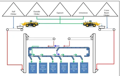
[image:12.595.101.500.406.659.2]

The chosen case study to implement identification of cement manufacturing raw materials using machine vision is on a tilt pan conveyor. This tilt pan conveyor transports clinker, gypsum and limestone to six storage bins which supply two cement mills. These raw materials are reclaimed from under storage sheds or manually loaded using a front end loader (22tonnes a load) into two loading hoppers from outside stockpiles. These two loading hoppers and reclaim conveyors transport raw materials to the tilt pan conveyor via two different conveying systems. These two conveying systems load their contents onto the tail end of the tilt pan conveyor system and the middle as shown in Figure 1. These materials then make their way to the desired bin by the operation of a diverter rail which allows the pans to tilt. The raw material can transfer from the top conveyor to lower conveyor or they can be directed to the desired bin. This system can deliver any two materials via the tail and centre transfer points. Through this clever design 1000 tonnes per hour (2 x 500 tonnes per hour) can be transported to the mill's storage bins.

Figure 1: Cement Manufacturing Raw Materials Transport System Overview

(13)

[image:13.595.101.496.69.403.2]

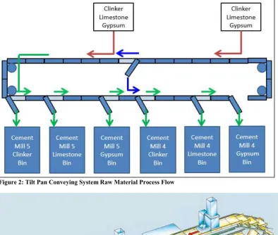
Figure 2: Tilt Pan Conveying System Raw Material Process Flow

(14)

1.3

Raw Materials to be Identified

1.3.1

Clinker

Portland clinker (shown in Figure 4) is made up of varying amounts of high-grade limestone, blended stone, silica (sand) and magnetite. Table 1 below shows the typical raw material contributions required to manufacture Portland clinker.

Figure 4: Image of Portland Clinker.

Table 1: Typical Raw Materials Used to Manufacture Clinker (Hewlett, 2016) Name Contribution Minimum

Clinker

Maximum Contribution to

Clinker

Chemical Formula

High Grade Limestone 9% 12% CaCO3

Blended Stone (Limestone) and

(Clay) 85%

93% CaCO3

7% Al2Si2(OH)4

Silica 0% 1.2% SiO2

Magnetite 0% 0.6% Fe3O4

Clinker is manufactured by feeding the three raw materials into a vertical roller mill or a ball mill. These mills grind the material down to the consistency of talcum powder which is called raw meal. This raw meal is transported to a cement kiln where the raw meal enters into the top of four series connected preheater cyclones. The raw meal enters the first riser duct where the hot kiln gasses move this material into enter the first cyclone. This first cyclone then separates the meal from the kiln gasses via a swirling centrifugal force (similar to the Dyson vacuum cleaner bag less dust bin). This meal then leaves the bottom of the first cyclone and drops into the second lower riser duct which leads to the second cyclone. This process repeats until the material enters the fourth cyclone where the meal enters the kiln.

(15)

knowledge of the topic. This clinker is then stored to be transported to the Cement Mill's when needed.

Clinker's contribution to the manufacture of cement is pivotal as it makes up more than 92.5% of the final cement product (Australian Stardards, 2010). This clinker in cement is responsible for the chemical reaction that takes place when water is added to make cement bond the aggregate to form the strong concrete structure. Too much clinker in Cement will cause the concrete to set too quick and not enough will cause the concrete to be too weak (Hewlett, 2016).

It is important to note that clinker contains up to 93% limestone which can makes it very similar in colour to limestone. When oversized clinker leaves the cooler, it also can be broken into shards similar to limestone by the cooler's clinker breaker.

1.3.2

Gypsum

Gypsum used onsite (see Figure 5) is a natural forming raw material supplied from mines in South Australia. They are transported to the site via ship, and then road transport. This raw material is then stored outside in 33,000-tonne stockpile on a concrete pad. This raw material is exposed to the weather which has a continuously varying moisture content. Gypsum is used to manufacture cement because it slows the chemical reaction that the clinker contributes to concrete. If too much gypsum is used the concrete will take too long to set and concrete expansion can occur. If not enough gypsum is used the concrete can flash set and become brittle, offering minimal strength (Hewlett, 2016).

One main point to note is that the chemical formula for gypsum is calcium sulphate dihydrate [CaSO4 2H2O] (Hewlett, 2016), and this has similar concentrations of Calcium

as clinker and limestone. The sulphate (SO4) contributes to the yellow colour which

offers a significant visible colour difference.

(16)

1.3.3

Limestone

Limestone used to make both clinker and cement is drilled, blasted, mined and crushed on a daily basis. All mined limestone is crushed then transported to an undercover storage shed in a 15,000-tonne stockpile. The blended stone (previously mentioned) is mined and crushed through the same system but stored in two undercover 35,000-tonne stockpiles. All limestone needed for the Cement Mills is manually transported from the stockpile and loaded into one of the two receival hoppers. The typical formula for limestone is CaCO3. This raw material has a similar colour spectrum to clinker which will contribute to the challenge of identification using colour. Limestone in cement manufacture has been used to improve the grind ability, reduce the thermal and electrical energy per tonne of the finished cement. Limestone is only allowed to be added to the cement process at maximum of concentration of 5% (Australian Stardards, 2010).

Figure 6: Image of Limestone

1.3.4

Cement

General purpose Portland cement is made by feeding clinker, gypsum and limestone into a wind-swept ball mill. The ball mill is a large cylinder divided into two the crushing chamber and the finishing chamber. These two chambers are filled with two different grades of mill balls varying from 110mm to 30mm. These ball mill rotates at a speed which allows the mill balls to be lifted up to two-thirds of the height of the mill and then drops down crushing the raw material. The raw material passes through the crushing chamber to the finishing chamber by the air passing through the mill. The grinding forces generate particle friction which also generates the heat required heat to dehydrate the raw material. This crushed raw material leaves the mill which is now called cement. This cement is transported to a separator which returns the oversized material to the mill inlet. The correctly sized material passes to the finished product transport system.

1.4

Raw Material Cross Contamination Impacts

(17)

1.4.1

Impact on Finished Concrete

Table 2 below shows a brief summary of the impacts to the finished concrete. Some conditions are complexly unacceptable and will lead to an entire day’s production being sent to land fill. These events have a severity listed as high. The medium and low impacts can be isolated, tested and blended back into the process at a very low dose rate for reprocessing.

Table 2: Concrete Impact Assessment Overview

Condition _ConsequenceImpact on Concrete 7 Day

Strength Strength Severity 28 Day

Too Much Clinker

>98%

Increased Risk of Flash Set Increased Risk of Cracking Not compliant with AS2350.4 Not compliant with AS3250.7

Decrease Decrease High

Not Enough Clinker <92.5%

Low Strength Will not Cure

Not compliant with AS3972 Not compliant with

AS/NZ2350.11

Too Much Gypsum

>2.8%

Slow Curing Time May not Cure

Increased Risk of E

xpansion

Not compliant with AS2350.14

Not Enough Gypsum

<2.6

Increased Risk of Flash Set Increased Risk of Cracking

Not compliant with AS2350.4 Decrease Decrease High

Too Much Limestone

>5%

Low Strength Will not Cure

Increased Risk of Sulphate Attack

Not compliant with AS3972

Decrease Decrease Medium

Not Enough Limestone

<5%

Increased Concrete Strength

Increased Variability Increase Increase Low

(18)

1.4.2

Operational Impacts

A summary of potential operational impacts has been listed below in Table 3. Some effects are completely undesirable for instance an increase in thermal and electrical energy consumption per tonne of cement produced would lead to wasted energy, more CO2 emissions and reduced profit margin.

Table 3: Operational Impact Assessment

Condition Consequence $/tonne

Thermal and Electrical Energy Too Much Clinker >98%

Clinker is the most expensive material Clinker requires most energy to make Open to litigation due to Concrete Fault End User Contract Variability Fine

Increase Increased

Not Enough Clinker <92.5%

Reduced material costs Reduced energy costs

More cement needed to maintain strength End User Contract Variability Fine

Decrease Decrease

Too Much Gypsum

>2.8%

Gypsum is the next most expensive Less energy needed to grind

Open to litigation due to Concrete Fault End User Contract Variability Fine

Increase Decrease

Not Enough Gypsum

<2.6

Other materials are harder to grind Open to litigation due to Concrete Fault

End User Contract Variability Fine Decrease Increase

Too Much Limestone

>5%

Open to litigation due to Sulphate Attack

End User Contract Variability Fine Decrease Decrease

Not Enough Limestone

<5%

Other raw materials are more expensive Clinker is harder to grind

End User Contract Variability Fine Increase Increase

Data has been summarised using sensitive operational data which cannot be shared

1.5

Existing Control Measures

1.5.1

Loader Operator

The front end loader operator is one source of cross contamination. As they load the raw materials into the hopper the system informs them what material to load. When they load the hopper with the requested raw material, there may still be another product in the hopper which may have bridged over and not gone through the system. From their position they cannot always see if the hopper is empty due to poor lighting, time constraints or other reasons.

1.5.2

Central Control Operator

(19)

which can lead to operator overload. With newer technologies operators have high-level control systems helping them cope, but they are still required to monitor 30 conveyor process cameras as a prevention against raw material cross contamination.

1.5.3

Process Attendant

Per shift, there are two process attendants and a shift quality tester. The process attendants conduct hourly walk arounds to inspect the plant and look out for

abnormalities in operation. These walk arounds are another form of raw material cross contamination prevention but they are unavailable during abnormal process conditions in other areas.

1.5.4

Conveying System Design

The conveying system design is an important cross contamination prevention system. Systems design should prevent material from bridging over, hanging up but due to legacy designs and process modifications these material hang-ups and material bridging occurs more frequently when raw material moisture changes. The control system is also a control measure which is used to prevent these events. Due to a lack of equipment maintenance due to restricted access time caused by the ever increasing demand for cement, it can be difficult to maintain this equipment at the desired frequency.

1.5.5

Conveyor Purge Time.

The control of the conveying system has a purge timer of 12 minutes between raw materials. This purge time forces the conveyor to run for 12 minutes without any material on the belt. This can waste up to 2 hours per day during peak production times. Not to mention the wasted energy, additional wear on the hardware and lost production opportunity (2 hours x 1000 tonnes per hour = 2000 tonnes in lost raw material delivery tonnes).

1.5.6

Quality Testing

(20)

1.6

Problem Statement

In the cement manufacturing industry, there is a need for a system which can identify raw materials as they are transported on conveying systems. Such a system will allow

automated identification of raw material as they are transported along common

conveying. This automated system can prevent cross-contamination before they occur by alerting the operator and sending a command to the control system which will stop the conveying system. The operator will have the opportunity to redirect the incorrectly loaded raw material to the correct storage location hence preventing a

cross-contamination event.

An automated raw material identification will need to;

 Identify the raw materials without the need to extract a sample from the

conveyor,

 Operate in an environment with varying lighting levels due to artificial lighting

and natural lighting,

 Not be affected by fugitive dust, vibration or localised sources of interference.

 The system must not affect conveying systems due to a failure,

 Identify each raw material in an acceptable time frame (less than 30 seconds as

280kg passes through the system every second),

 Able to identify raw materials with a high level of confidence.

1.7

This Project’s Proposed Contribution to the Gap in the

Literature

(21)

1.8

Dissertations Overview

Chapter One – Introduction

The opening chapter of this dissertation covers an in-depth overview of the layout of the chosen case study. This overview will help the reader to understand the motivation behind the project and the problem the project intends to resolve.

Chapter Two – Background

A literature review was conducted and continuously reviewed as new problems presented themselves. This continual literature review also identified the way in which this body of work will contribute to the available literature.

Chapter Three – Methodology

The methodology chapter presents the process which was followed to design, build, test, optimise and verify the developed model. This provides an in-depth understanding of how the research cycle was used to ensure the project’s objectives were delivered.

Chapter Four – System Development

Chapter four provides an understanding of how the initial model and system was developed and documents the engineering decisions which were made.

Chapter Five – Model Optimisation

The initial systems development was tested, and opportunities were found during a reflection of initial results and a review of the literature. This chapter covers the improvements that were implemented to model.

Chapter Six – Results and Analysis

A reflective review and analysis of the results were documented in this chapter. Critical analysis of the available testing data and comparison of the initial model’s performance against the optimised models performance will be presented.

Chapter Seven – Conclusion and Further Work

Finally, a summary of the projects achievements, opportunities for future model improvements and how this body of work can improved in the future.

1.9

Intellectual Property Disclaimer

(22)

2

Background

2.1

Overview

The literature review has been broken down into several subsections which offer a logical breakdown of the primary tasks of this project. The first subject will discuss the

importance of sample selection and collection to ensure an accurate representation of all raw material are sampled. The second section discusses the important attributes of camera sensor types which are available for use in the industrial environment. This same section also discusses the different lighting technologies and methods which will offer the best outcome.

The next section will discuss image pre-processing requirements to ensure the image is submitted to the feature extraction system free from noise. From the image, pre-processing feature extraction will be the next section which covers colour and shape features. The last portion of this subsection discusses the ways which raw materials can be classified using statistical and decision ruling algorithms.

2.2

Sample Selection and Collection

The importance of sample selection and collection should not be underestimated. To ensure an accurate representative sample is acquired from the raw material sample location work conducted by (Chatterjee & Bhattacherjee, 2011) and, (Hamzeloo, et al., 2014) took their samples from conveyor belts, stockpiles and blast sites using Stratified Random Sampling. This Stratified Random Sampling method divides the total population (total tonnes in the stockpile, total production time or, expected total production tonnage) by the required number of samples required. Once the stratification start and finish points are known a random number is generated to determine the sample location along a stockpile or to sample at a particular produced tonnage.

= × ( − + ) ( 2-1)

Where S is the stratification size, is the current sample increment and R is the random generated number between 0 and 1. Equation obtained from (Australian Standards, 2012a). One key point to note is that a random seed be used for the generation of the random number.

2.3

Image Acquisition

2.3.1

Camera Sensor Types

The selection of the camera sensor type is a critical aspect of the project as an accurate representation of the raw material must be presented to the feature extraction system. Images submitted to the feature extraction system must be free of shape distortion from a picture taken from a moving conveying system. Shape distortion happens when a

(23)

Figure 7: Pixel Scanning with Rolling Shutter – Image obtained from (Nakamura, 2006)

Figure 8: Illustration of shape distortion of moving objects in a rolling shutter

To avoid this situation work conducted by (Mkwelo, 2004), (Selver, et al., 2011) and, (Isa, et al., 2011) selected a camera using charged-coupled device (CCD) camera. To understand the importance of a CCD, a summary of the technical operation obtained from (Nakamura, 2006) has been provided in the following subsection. A comprehensive review has been conducted where we will also investigate the available literature on Complementary Metal-Oxide Semiconductors with global shutter functionality. This design has been created to eliminate the problem with shape distortion.

Charged Coupled Device (CCD) with Mechanical Shutter

Figure 9 below shows a cross section of a second generation interline transfer CCD for a single pixel. The CCD sensor array is exposed to the light (photons) which passes through the lens to by the opening and closing of a mechanical shutter for a

(24)

until all rows have been processed. Once this process is complete, then all components have reverted to a zero state charge ready for the next image (Nakamura, 2006).

Figure 9: Cross Section of Second Generation Interline Transfer CCD - (Nakamura, 2006) Global Shutter Complementary Metal-Oxide Semiconductor (CMOS)

A rolling shutter CMOS sensor has been shown in Figure 7 above. This system can work with a shutter, but typically the shutter is an electronic function where the individual pixel image circuitry is turned on when required. The circuit shown in Figure 10 is a CMOS Rolling Shutter typical circuit. When the shutter/exposure time has been activated a pulse is sent to the Gate of transistor MRS where the photodiode and the Gate of transistor MRD are pulled up to the reset voltage. Then a pulse width of the required exposure time is sent to the gate of Transistor MSEL where the voltage potential from the exposure of light to the photodiode is forwarded to the analogue to digital converter. Each pixel is processed starting with Row 0 Column 0, then Row 0 Column 1 until the end of the row pixel has been processed then the next row will be treated the same way until the full pixel array has been processed. This explanation of the process is the reason why CMOS rolling shutter sensors are subject to shape distortion of moving objects (Nakamura, 2006).

In recent years CMOS sensor manufacturers have found solutions to the shape distortion of moving objects problem by the advent of the CMOS Global Shuter. The CMOS global shutter incorporates technology which allows the individual CMOS pixels to store their electrons similar to CCD sensors (Demant, et al., 2013). With the implementation of this Global shutter technology, more cost effective industrial sensors can be constructed which are less subject to noise and interference.

(25)

2.3.2

Lighting

The chosen lighting method for illuminating the image for raw material identification is an important feature to consider. Machine vision lighting for the application of our application should consider (Martin, 2007);

 Ambient Lighting Contributions,

 Lighting Source (Fluorescent, Quartz Halogen, LED, Metal Halide, Xenon)

 Lighting Wavelength (Visual Range 400 to 650nm)

 Illumination Techniques (Back Lighting, Diffuse Lighting, Bright Field, Dark

Field)

With these considerations, we will briefly discuss these items concerning the literature review.

Ambient Lighting Contributions

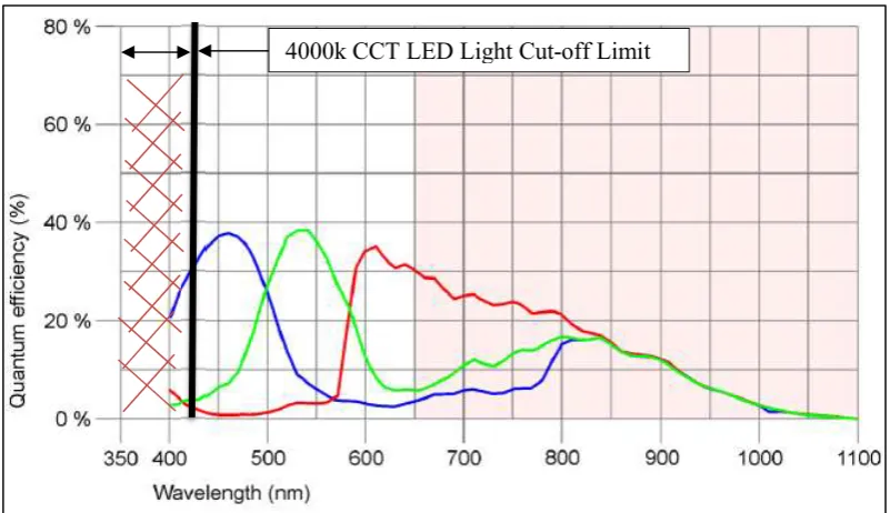
To be able to identify each raw material repeatedly we will need to ensure sources of ambient lighting do not affect our sampled image. These variations in ambient lighting can stem from natural lighting, area lighting and in our case high pressure sodium lighting. Each of these lighting sources offers image variability due to their varying wavelength intensity (Martin, 2007) which can be seen in Figure 11 below.

Figure 11: Light Source Relative Intensity Verses Spectral Content obtained from (Martin, 2007)

Work conducted by (Patel & Chatterjee, 2016), (Cunha, et al., 2015) and, (Selver, et al., 2011) managed this ambient lighting variability by installing their camera in a controlled lighting enclosure. This allows lighting to be controlled in a manner which will ensure stable lighting.

Controlled Lighting Source

(26)

subtraction model. This lighting intensity model was able to be subtracted from a sampled image to remove this effect. In most lighting source applications there will be sources of non-laminar lighting. This method allows the image to be sampled with minimised effect from the light sources.

Figure 12: Effect of Xeon Lighting obtained from (Cunha, et al., 2015)

An additional consideration is the lighting enclosures internal surface preparation. The controlled light source in (Chatterjee, 2013) paper was the use of fluorescent lighting, but they also prepared the inner surfaces of their lighting enclosure with white magnesium oxide. The reasoning behind this was to apply uniform diffuse ligh to their application which allows an even lighting on their raw material.

In contrast to the diffuse lighting work by (Selver, et al., 2011) their lighting enclosure was painted black to minimise unwanted reflections. The image selection method conducted by (Cunha, et al., 2015) was also replicated in (Chatterjee, 2013) and (Selver, et al., 2011). This image lighting intensity subtraction model negates the importance of internal enclosure finish.

Illumination Techniques

The importance of image illumination technique will become apparent in the following explanation of the various illumination techniques. The common machine illumination techniques obtained from (Martin, 2007) are listed below;

 Backlighting,

 Diffuse Lighting,

 Bright Field

 Dark Field

(27)

Diffuse and Dark Field Lighting

The dome diffuse method is the most realistic application of diffuse lighting in which we could implement. Figure 13 shows, an example of dome diffuse lighting. An application of this technique can be seen in (Chatterjee, 2013) which was explained above where they achieved this diffused dome lighting by painting the internals of their lighting enclosure with the white magnesium oxide. This application positioned their lighting in the dark field illumination position. Their intention was to access the benefits of both techniques where the image would not be saturated so a good representation of colour would be available but also the dark field lighting minimises shadows (Chatterjee, et al., 2010).

Figure 13: Dome Diffuse, Bright Field and, Dark Field Illumination obtained from (Martin, 2007) Bright field Lighting

Bright field lighting applications are usually applied where user wants to enhance topographic detail (Martin, 2007). From Figure 13 we can see the lighting source is nearly perpendicular to the image surface. This method is particularly handy where a watershed image segmentation algorithm will be used to find raw material edges for raw material sizing purposes. This method has been utilised in the work conducted by

(Mkwelo, 2004) where he placed his lighting in a high incidence angle to his raw material to encourage the shadows around his limestone to allow better image segmentation.

2.4

Image Pre-processing

There are multiple methods to pre-process images before they are presented to the image segmentation and feature extraction. In work by (Chatterjee, et al., 2010) and, (Selver, et al., 2011)they considered the average and median filters to remove unwanted noise in their images. They implemented the median filter which is capable of eliminating input noise values of extremely high values. Due to the importance of a median filter, a brief explanation will be presented in the proceeding sub-section.

Median Filter

(28)

Figure 14: Operations involved in a median filter, method adopted from (Davies, 2012)

Figure 15: Filter Functions Compared, obtained from (MathWorks, 2016) Figure 15 Explanation

Photo A: MATLAB Original Image

Photo B: MATLAB Original Image with Salt and Pepper Noise added Photo C: MATLAB Noisy image with Average Filter applied Photo D: MATLAB Noisy image with Median Filter applied

Average Filter

(29)

Figure 16: Operations Involved in an Average Filter, method adopted from (Davies, 2012)

2.5

Feature Extraction

For the identification of raw materials, there is a broad range of features which we can extract from our pre-processed image. The most relevant feature extraction methods will be explained in detail, and the review literature will support the importance of these methods. To enable an organised presentation of this material all considered features will be categorised under colour and shape properties.

2.5.1

Colour Features

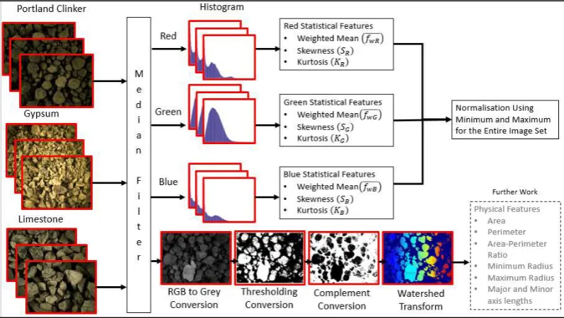
From our sampled image we can extract multiple colour features. Work conducted by (Chatterjee, et al., 2010), (Tessier, et al., 2007), (Shanmugamani, et al., 2015) and (Wang & Li, 2015) all used colour in the identification of their raw materials. They achieved this by converting each of the Red, Green and Blue components of a pre-processed image and depending on the image colour depth create a histogram. In these cases, the colour depth was 24bit which means Red, Green and, blue all are represented by 8 bits or 255 intensity levels for each colour. This will require 255 bins to count each of the individual intensity levels. This histogram of each colour was then passed through a statistical algorithm which would determine the weighted average, skewness and kurtosis of each colour. This created nine individual features from three colours (shown in Figure 17 below). The equation to calculate the weighted average, skewness and kurtosis have been listed below in equations ( 2-2 ) to ( 2-6 )

=∑−= × ( )

∑−

= ( 2-2 )

Where the weighted mean, f is the pixel intensity, H represents the histogram of the

image, L is the number of pixels’ intensities in the image. Equation obtained from (Patel & Chatterjee, 2016)

=∑−= × ( )

× ( 2-3 )

=∑ _× × ( ) ( 2-4 )

= × ∑ × ( )

√ ( 2-5 )

= × ∑ × ( )

(30)

Where ̅ is the mean, v is the variance, s is the skewness and k is the kurtosis, p is the total horizontal pixels, q is the total vertical pixels. Equations (1.3) to (1.6) also are obtained from (Patel & Chatterjee, 2016)

Figure 17: Colour Feature Extraction obtained from (Patel & Chatterjee, 2016)

To add to these colour features (Chatterjee, 2013) also converted the pre-processed images to Hue, Saturation, Intensity and Grey. These additional histograms were then passed through statistical location (median, mode), the measure of spread (variance, standard deviation, range, mean absolute deviation, interquartile range) (Chatterjee, 2013). This work per image would extract a total of individual 70 statistical colour features (7 colour attributes x 10 statistical features). This appears to be excessive, but at the same time, it does allow multiple paths to move on in the event of an unacceptable raw material identification rate.

2.5.2

Shape Features

Another method which can be used to identify raw materials is shape features as these features are unique to most raw materials. Shape features are not as readily available as colour features as they need to be passed through an image segmentation process. This process was repeated by (Chatterjee, 2013), (Mehrabi, et al., 2014), (Mkwelo, 2004), (Thurley, 2011) and, (Andersson, et al., 2012) where the image is modified in the order shown below;

 Original Image Sampled

 Filtered

 Grey Scale Conversion

 Image Thresholding

 Image Complement

 Distance Transformation

 Watershed

(31)

Steps 1 to 3 are standard functions and have already been explained. The image thresholding is a process where the image is converted from a grey scale image to a binary image. Then the image complement is created using the threshold binary image, and all the ones are changed to a zero and vice versa (Davies, 2012). Finally, the distance transform and the Image Complement are combined and submitted to the watershed algorithm. The watershed transform treats the images as a topographical map where each pixel’s grey intensity represents the height of the individual pixel. The lowest point of the image is effectively flooded one intensity level at a time. Points, where the water was to spill into a valley, are marked as an edge/dam wall. This dam wall pixel is set to positive infinity. This will then continue to flood the image to the next spill point where this is also marked as a dam wall. This process continues until the image is fully flooded the maximum field intensity. All the dam walls are declared the watershed image lines (Mkwelo, 2004).

In (Mkwelo, 2004) work he tested a marker-based watershed segmentation process which provided to be far more accurate than the other segmentation methods (e.g. canny filter, Opening and Closing). For more information on the other filter types refer to (Davies, 2012) or (Mkwelo, 2004).

From this segmented image, we can obtain the measurements of the individual raw material particles which will allow us to extract the features listed below which were obtained from (Davies, 2012), (Chatterjee, 2013).

 Area,

 Perimeter

 Area-Perimeter Ratio

 Minimum Radius

 Maximum Radius

 Major and Minor axis lengths

2.6

Material Classification

The main methods used to classify raw materials in the reviewed literature are the Probabilistic Neural Networks and, Multiclass support vector machines. Both these methods can operate in the supervised and unsupervised states. The Probabilistic Neural Network (PNN) implemented by (Patel & Chatterjee, 2016) (depicted in Figure 18) consists of a feature database consisting weighted average, skewness and kurtosis of each colour (further explained in section 2.5.1 above) are submitted to the input layer. These features are entered into input vector X shown in equation 7) below. From equation (2-7) the input vector is entered into Equation (2-8) to form the pattern layer where the neurons are divided into a number of classes C (Patel & Chatterjee, 2016). This result is then fed into equation (2-9) which forms the summation layer classes. Finally, the results of equation (2-9) are passed to the final equation (2-10) which determines the class the input image best represents. This process is repeated for all training photos to ensure the system has the required data to identify each material. Equation (1-7) to (1-10) below were obtained from (Patel & Chatterjee, 2016)

= , , , ∈ , = = ( , , ) ( 2-7 )

,( ) = − , ( 2-8 )

( ) = ∑ ,( ) , ∈ , , … ( 2-9 )

( ) = ( ) ( 2-10)

Where is the image vector;

(32)

is the skewness is the kurtosis , ( ) is the pattern neuron

is the smoothing parameter is the number of training images

( ) is the summation layer

( ) is the output layer

Figure 18: Probabilistic Neural Network, obtained from (Patel & Chatterjee, 2016)

To test the PNN success rate (Patel & Chatterjee, 2016) created a Matching matrix to determine the success rate. This matrix compares the actual image against how many images were miss-classified.

(33)

3

Methodology

3.1

Project Approach

This research project will demonstrate a quantitative research approach which will follow the stages of the research cycle shown below in Figure 19. This approach developed the research questions which will be used to guide the literature review. From this literature review, a gap in the literature will be found and potential techniques. This will provide the required information needed to build and test and evaluate a model's performance Also a test rig or program will provide a quantitative evaluation of the systems resultant data. This evaluation will offer the required data which will allow analysis of the results and which will lead into the critical thinking phase. This critical thinking phase will allow a review of the results to determine if the desired outcome has been delivered. It will most likely lead to a review of the research questions or so a revisit of the literature can occur to find improved ways to optimise the model. This research process can undertake many cycles to deliver the desired result.

Figure 19: Project Research Cycle adopted from (Maxwell, 2016)

3.2

Overview

This project will involve the construction of a camera enclosure and test bed. The camera enclosure and test bed will be used to design a material classification model. This

classification model will need to be able to take a significant number of still images with a camera. A computer-based system will be used to extract unique features from the image. These image features will be used to classify the raw material present in the image.

Research Question

Background

• The things that you know

Literature Review

• To find the Gap

Address the Gap

• Optimise

• Performance over cost, • Reduce operator stress

Evaluation Criteria

• Test Program

Results Analysis

• Basic Analysis • Statistical

• Software Package Analysis

Critical Thinking

(34)

For this research project, the scope is to design, test and optimise a static model with the future intention (after the dissertation is complete) to implement this model on a live conveying system which will be able to optimise itself and operate in the operational environment dynamically. With this in mind, all future design considerations and project work will consider the needs of the static model development and the proposed dynamic functional model.

3.3

Sample Selection and Collection

To be able to take training and verification images the three raw materials will need to be collected. These raw materials will also need to be sampled in a manner which will ensure an accurate cross representative sample is taken from the stockpiles and process which also will represent the total body of raw materials which the process will consume for the development life of the project (May 2016 to October 2016). Sample storage considerations should address ways in which the sample will maintain moisture content present when extracted and can be made available for future quality or physical analysis should this be needed.

3.4

Training and Verification Image Acquisition

To be able to take training images a camera will need to be selected and purchased. A Camera enclosure, camera lighting system will need to be designed and constructed. The design of the camera enclosure and lighting system will need to be developed to address the needs of static operation and meet the needs of the future dynamic system. As well a test bed will be necessary to place the samples on to take the required training and verification image acquisition. Since the future dynamic model will need to operate over the tilt pan conveying system shown in Figure 2 and Figure 3 a spare tilt pan will be used as the test bed. The test bed will hold the raw material samples used to take the training and verification images.

3.5

Image Pre-Processing

Once the training and verification images have been taken, we will need to ensure the images are free from noise and image pixel saturation. It will be important to pass the images through a filter as the wet raw material will be highly reflective and may cause localised image pixels to become saturated.

3.6

Image Feature Extraction

From the taken training and verification images we will need to determine quantifiable features which will be unique to each raw material. For automated classification using these image features, we will require several unique features for all images to improve the classification model's success rate. Additionally, chosen image features will need to consider the processing time taken to extract each images features. This processing time consideration will need to ensure a picture can be classified within the problem

statements goal of thirty seconds.

3.7

Material Classification

(35)

developed using a mixture of C# programming for the application layer and dotNET coding for the camera control.

3.8

Model Performance Evaluation and Optimisation

(36)

4

System Development

4.1

System Design Considerations

The system development considered all aspects of the proposed systems lifecycle. For this dissertation, the model developed was a static system used to build, test and optimise the developed model in a controlled environment. This static system will allow the model to be developed free from the operational environment. To minimise waste, the hardware will also be used to conduct static system evaluation and designed to address the dynamic system needs.

The operational environment where the future dynamic system will be installed will subject the system to fugitive dust, varying ambient light, temperature variations and moisture variations. The systems shall not impact the sites conveying system as this will be an unacceptable outcome.

4.2

Overview

The first step in this project system development will discuss the method developed to sample the raw materials. The next development discussion point will be the selection of camera, design of the enclosure and discussion surrounding the selection lighting. The following point of discussion will be the way in which the images were taken and then had their features extracted. Finally, the probabilistic neural network model development and verification consideration will have been discussed. An overview of this process has been provided in Figure 20 below.

(37)

4.3

Raw Material Sampling

4.3.1

Overview

The work conducted by (Chatterjee, et al., 2010) and (Hamzeloo, et al., 2014) clearly outlines the importance of developing a sampling plan which will extract a true

representative sample of the raw material population your wish to sample. This sampling importance has been explained in detail in section 2.2. In their case, they used Stratified Random Sampling, which is a procedure which divides a total population (Total Length of a Stockpile, Total Production Time or, Total Tonnes Produced) by the number of Increments. ( (Australian Standards, 2012a) states there are five increments per sample). Once the number of required increments and the total population is known, equation (4-1) below can be used to determine the exact location of each increment (length along a stockpile, point in production time or tonnage produced) will need to be extracted from.

= × ( − 1 + ) ( 4-1 )

Where is Total length in [m], for Total Length Stratification;

is Total time in [hours], for Total Production Time Stratification; is Total length in [t], for Total Tonnage Produced Stratification; is the Increment Number;

is the Randomly Generated Number which will be between 0 and 1. In (Australian Standards, 2012a) it clearly states that procedures developed using this series is only to be developed by a person who is experienced and qualified in geological engineering. This advice will not be adhered to as access to such an engineer is not available and this standard is only being used for its Stratified Random Sampling

procedure. If the samples acquired for this project were to be used for quality analysis, we would need to approach such an engineer. Given the nature of this work we will not consider use of such an engineer and list this item in our project limitations.

Work by (Chatterjee, et al., 2010) claimed that at least 100 images of each sample are needed totalling 500 images per raw material. For this project five samples were extracted for each raw material is based upon the need to generate at least 100 imaged for each sample from the above mentioned work.

4.3.2

Clinker

The work by (Chatterjee, et al., 2010) and (Hamzeloo, et al., 2014) was not conducted in Australia. There is a standard for implementing Stratified Random sampling and this standard is (Australian Standards, 2012a). This standard’s scope covers all raw material particle sizes up to 63mm. For clinker all historical sizing conducted onsite were obtained and the particle size distributions have been listed in Table 4.This data is obtained by mechanically sifting the raw materials through a series of sieves with the aperture listed below in the table as particle size in millimetre measurements. The number listed under minimum, average and maximum columns are the percentage weight each particle size class is of the total samples weight (e.g. 30.34% represents the maximum portion of particles measured in 10 years were in the 19.1mm particle range).

(38)

Note: 2D represents greater than 90mm in 2 dimensions and 1D only greater the 90mm in one dimension.

With the use of table 4 we can see that our largest recorded clinker particle size was 38.1mm and according to table 5 from (Australian Standards, 2012a) we can see that the clinker sampling procedure will need a minimum increment mass of 6kg and a sample size minimum of 30kg.

The clinker on site is continuously manufactured and only stored for a short time before it is consumed in the cement mills. For this reason, our sampling procedure will be a tonnes produced stratification. During the projects life time, from May 2016 to October 2016 665,160 tonnes will be produced. So equation ( 4-1 ) will be used to stratify the tonnes produced and it has been decided upon an educated guess that we will require we will require 5 samples which will consist of 25 increments in total.

The detailed procedure, stratification of increments recording and sampling has been provided in Appendix N, O and P.

Table 5: Minimum Increment and Sample Mass, Data obtained from (Australian Standards, 2012a) Nominal Size,

mm 90 75 40 28 20 14 10 7 5 <5

Minimum mass

per increment, kg 12 10 6 5 4 3 2 2 1 1

Minimum Mass

per Sample, kg 59 50 30 25 20 15 10 10 5 5

To find the values for 90 mm which has been highlighted in yellow we will need to extrapolate the data using equations ( 4-2 ) to ( 4-7 ) obtained from (James, 2010).

= = = 0.1143 ( 4-2 )

= = = 0.5714 ( 4-3 )

Where is the highest known y axis value, is the next highest known y axis value,

(39)

ℎ ℎ ℎ

Substitute ( 4-2 ) into ( 4-3 ) to determine

= × + ( 4-4 )

10 = 0.1143 × 75 +

= 1.4275

= × ( 4-5 )

50 = 0.5714 × 75 +

= 7.145

Where Y is the extrapolated data

is the unknown x axis data point is the x=0 y intercept point.

With this in mind we can generate our linear equation which we will used to extrapolate our increment and sample mass for particle size equals 90mm. This has been shown in equation ( 4-6 ) and ( 4-7 ) below.

= × + = 0.1143 × 90 + 1.4275 = 11.7 ( 4-6 )

= × + = 0.5714 × 90 + 7.145 = 58.57 ( 4-7 ) The Clinker was sampled was directly sampled off the conveyor at the stratified tonnes produced increments listed in Appendix N. The conveyor was not to be stopped as this would lead to a production stop. All materials were sampled at a purpose built sampling station shown in Figure 21 which has all the conveyor draw in hazards engineered out. Another point to note is that the temperature of the Clinker travelling up the conveyor varies from 200°C to 500°C. For this reason, a high temperature protective apron, gloves and face shield were worn during sampling. As well all clinker was placed into a steel bucket using a long handled sample scoop (to minimise the conveyor draw in risk).

(40)

4.3.3

Gypsum

Gypsum is a product which is shipped to site from South Australia in 36,000 tonne shipments. This raw material is delivered to site and stored on a large outdoor concrete pad shown in Figure 22. This stock pile was stratified up into 25 increments using

equation (4-1). This has all been recorded in Appendix O – Gypsum Sampling Procedure. The Australian standard (Australian Standards, 2012a) which was used to develop this procedure states that a stock pile is best sampled from the back of the truck as this stockpile is being constructed. In our case this stockpile was constructed before this project started. So to ensure the best representative sample was acquired the sample was extracted from the stock pile using a stockpile shield (see Figure 23) to a depth of 200mm plus the depth of the deepest measured effect of weathering (300mm which can be seen in Figure 22). With this in mind the increment was extracted from a depth of 500mm.

Figure 22: 33,000tonne Gypsum Stockpile

Figure 23: Gypsum Sampling using Stockpile Shield and sample scoop

(41)

Table 6: Case Study’s site 10 Year Gypsum Distribution analysis.

These increments were sampled from the stockpile using two people as risk of

engulfment was prevalent due to the piles extreme height of 35.8 meters and an angle of 38° Another point to note is that the standard requires the stock pile stratification

increment point to use length as well as the width of the pile. The length stratification was used but the width was not possible as an elevated work platform was not available for the task and to scale the pile to extract the sample was far too unsafe. All sampling details and considerations have been listed in Appendix O – Gypsum Sampling Procedure.

Figure 24: Stored Sampled Gypsum

4.3.4

Limestone

From Table 7 one very important point to note is that limestone has material larger than 90mm. This means that it will not be covered under the scope of (Australian Standards, 2012a) as this standard only covers up to 75mm particle size. Another point for

consideration is that the standard which covers these size particles is (Australian

(42)

maximum limestone particle size is 90mm. This can then be used find our increment mass of 12kg and total sample mass of 60kg using Table 5.

Table 7: Case Study’s site 10 Year Limestone Distribution analysis.

The limestone increments were sampled directly of the conveyor similar to the way in which clinker was sampled in subsection 4.3.2. The difference is the limestone increment was taked directly off the belt with the belt stopped and isolated. This allows the best possible sample to be taken as the entire cross section of the belt can be extracted (shown in Figure 25).

Figure 25: Limestone conveyor sampling

4.4

Camera System Design

(43)

 Be capable of being disassembled so it can be safely transported between the training image work area and the tilt pan conveyor by hand,

 No section of the of the disassembled system shall weigh in excess of 10kg due to

manual handling issues identified in the risk management plan in section Appendix B – Project Management Plan

 All surfaces must be painted black as per the discussion in section 2.3.

 Camera mount must be adjustable and be able to be locked into position

 Be designed to prevent conveyor material surges from striking the enclosure

 Minimise the effect of fugitive dust problems by ensuring the internals are kept

under filtered positive pressure

 Designed to be positioned on the tilt pan conveyor support frame and be

positioned on the concrete floor for image training purposes

4.4.1

Camera and Lighting Enclosure

Since the camera enclosure has to be able to operate in both the model development and operational phases the enclosure will need to be able to be installed over the Tilt Pan Conveyor’s operational structure shown in Figure 26. To put this figure into prospective the top of the pan to the floor level is 2260mm. The enclosures proposed location has been shown in this image by the red overlay. This location is the only location on this conveyor where such an enclosure can be installed. It would be ideal to be further away from the conveyor transfer point identified by the green ellipse shown below. This transfer point can be a main source of fugitive dust as material is falling from 5 meters above this area on to the Tilt Pan Conveyor. There is dust collection associated with transfer point but it only works when the material flow has been established and coming out the full height of the transfer exit point.

(44)

Camera Enclosure Support Structure

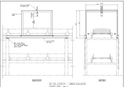
The proposed support location for the cameras structural channel has been shown in Figure 27. This location has been chosen for two reasons. The first is that it has the largest clearance between the Tilt Pan Conveyors haulage chain and the second is that it has the ideal support structure to mount our structural channel. The main two structural channels were selected using the help of the sites Structural Design Engineer Leigh Wiseman. Leigh’s support was requested as the span of 3600mm and the enclosure’s total weight was well out of the engineering abilities of the Author. Figure 29 shows two up right support channels where the top section will have a 10mm pad welded onto the top to hold down the camera enclosure’s support channel. Full detailed drawings have been provided in Appendix C – Enclosure Design Drawings and an image of the constructed unit can be seen in Figure 30.

Figure 27: Support Structure required clearance distance

Camera Support Bracket

The Camera enclosure design overview can be seen below in Figure 29. From this we can see the importance of the camera’s distance to the conveyed raw material. For this reason, the camera’s support bracket was stiffened to prevent undue camera vibration, far enough away from the raw material to prevent damage to the camera. Also the camera support bracket was designed to offer 150mm of height adjustment to allow manual camera focusing from outside the enclosure.

Camera Enclosure Dimensions

(45)

the position of the lights must be as close to the camera and far away as possible from the raw material as possible. The second consideration for enclosure height was the available clearance between the camera and the building’s roof (shown in Figure 28). The

enclosures height has been made as high as possible without interfering with the roof. Selection of the camera enclosures width is a clear decision to make as it governed by the Tilt Pan Conveyor’s dimensions. The length of the camera enclosure is determined by the camera’s field of view and the chosen lightings maximum length.

Figure 28: Camera Enclosure showing roof clearances

Enclosure Colour

Since Bright Field lighting (explained in 2.3.2) is being implemented it is important that no lighting reflections come from the enclosures internal surfaces. For this reason, all surfaces and internal materials shall be painted black.

Enclosure Construction

(46)

[image:46.595.100.500.59.339.2]

Figure 29: Tilt Pan Camera Enclosure Design Overview

Figure 30: Finished Camera Enclosure

4.4.2

Camera

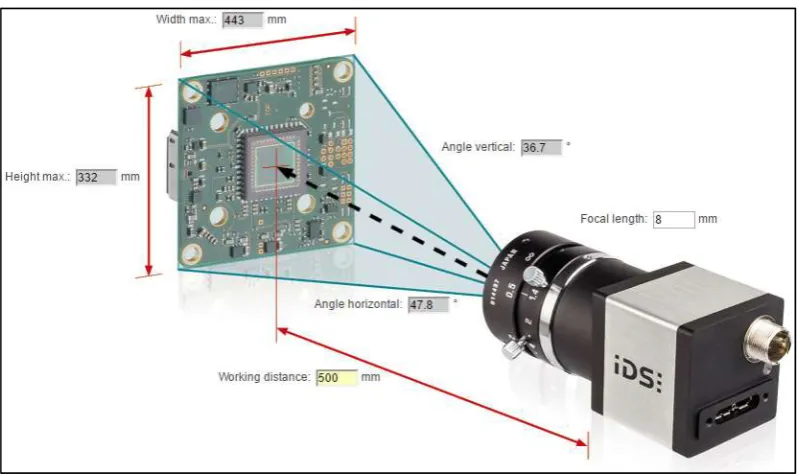
Image Size

Since the tilt pan conveyor pan maximum measured width is 835mm we are able to draw the conclusion that the largest image which can be sampled using a photo with a 4:3 aspect ratio Image dimensions will be 800mm x 600mm. With this in mind we are able to consider the required camera resolution with consideration to the desired Spatial

Calibration Resolution. Table 8 below shows the effect of physical image size

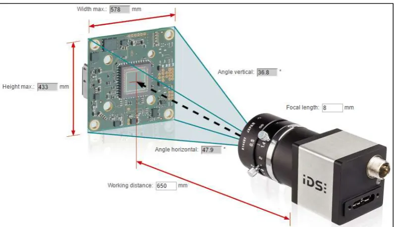
[image:46.595.101.393.360.592.2]

(47)

image which will have the desired resolution yet be able to see enough of the physical raw material for identification purposes.

With the selected lens in subsection 4.4.2 camera lens we selected a lens which should have given us an image 332mm High and 443mm Wide. This was not the case as the provided lens did not screw into the camera body appropriately which modified the desired focal lengths and ended up providing an image with 113mm wide by 150mm high. This is not desired but due to time constraints and the need to progress the project we continued with this modified focal range. Tests using 5mm grid paper were conducted to ensure the image was not distorted. The resultant resolution and image size has been highlighted in yellow below in Table 8: Image Pixel Count Related to Field of View Dimensions.

Table 8: Image Pixel Count Related to Field of View Dimensions

Image

Height Width Image

Spatial Calibration

Resolution (mm/pixel)

Pixel Count Image Size (megapixels)

600 800

0.1 4,800,000 4.8MP

0.15 3,200,000 3.2MP

0.2 2,400,000 2.4MP

0.5 960,000 0.96MP

450 600

0.1 2,700,000 2.7MP

0.15 1,800,000 1.8MP

0.2 1,350.000 1.35MP

0

Identification of cement manufacturing raw materials using machine vision

University of Southern Queensland

University of Southern Queensland

contained within or associated with this dissertation.

assessment in any other course or institution, except where speciﬁcally stated.

Contents

List of Figures

List of Tables

Glossary

Introduction

Conveying System

Raw Materials to be Identified

Gypsum

Limestone

Raw Material Cross Contamination Impacts

xpansion

Operational Impacts

Existing Control Measures

Central Control Operator

Conveying System Design

Quality Testing

This Project’s Proposed Contribution to the Gap in the

Intellectual Property Disclaimer

Sample Selection and Collection

Image Acquisition

Lighting

Image Pre-processing

Feature Extraction

Shape Features

Material Classification

Methodology

Overview

Sample Selection and Collection

Image Pre-Processing

Material Classification

Overview

Overview

Clinker

Gypsum

Limestone

Camera System Design

Camera and Lighting Enclosure

Camera